 Eldar Baykiev
 Mattia Guerri
 Javier Fullea
95% of researchers rate our articles as excellent or good
Learn more about the work of our research integrity team to safeguard the quality of each article we publish.
Find out more
ORIGINAL RESEARCH article
Front. Earth Sci. , 23 October 2018
Sec. Geomagnetism and Paleomagnetism
Volume 6 - 2018 | https://doi.org/10.3389/feart.2018.00165
In this work, we study the lithospheric structure of the British Isles using a methodology that allows for forward modeling of the Curie temperature depth based on seismic, elevation and gravity observations within an integrated geophysical-petrological approach (LitMod3D). We compute 3D thermal models and self-consistently determine the density in the mantle based on temperature, pressure, and bulk composition. Finally, we derive Curie temperature depth maps and forward calculate magnetic anomalies at the airborne level (5 km altitude) using a spherical magnetic modeling software (magnetic tesseroids) to estimate the geothermal magnetic signal. Our results show lateral lithospheric variations across the model domain, with Great Britain being characterized in general by thicker and colder lithosphere, especially in the south-east, and the thinnest and warmest lithosphere being located beneath west Scotland, Northern Ireland and in the north-west oceanic area. Our estimated Curie temperature depth map resembles the values obtained using other techniques (spectral method and surface heat flow inversion) in some areas, but discrepancies are notable in general. We determine that the effect of typical lateral temperature variations (i.e., Curie isotherm depth) accounts for 5–15%, on average, and up to 70% locally of the crustal magnetic signal at the airborne level. Our lithospheric models are in general agreement with published seismic tomography models as well as other geophysical studies.
Gravity data (Bouguer, free air or geoid anomalies) have been extensively used to image the lithospheric and upper mantle density structure (e.g., Götze et al., 1994; Kaban et al., 1999; Ebbing et al., 2006; Chappell and Kusznir, 2008; Maystrenko and Scheck-Wenderoth, 2013). More recently, gravity gradient tensor data measured at satellite height have been employed to image lithospheric and upper mantle density variations (e.g., Ebbing et al., 2013, 2014; Panet et al., 2014; Álvarez et al., 2015; Fullea et al., 2015). One of the main limitations of gravity data inversion/forward modeling is non-uniqueness. One of the strategies to alleviate such a problem is to simultaneously model various gravity data (e.g., gravity and geoid anomalies) and/or other geophysical datasets with complementary sensitivity (e.g., elevation and heat flow data; Zeyen and Fernàndez, 1994; Torne et al., 2000; Fullea et al., 2006, 2007), or gravity and seismic tomography data (e.g., Root et al., 2017). A more complex way is to jointly model or to invert gravity and other data sets within an integrated geophysical-petrological framework where the parameter space is redefined in terms of temperature and composition of rocks (e.g., Khan et al., 2007; Afonso et al., 2008; Fullea et al., 2009).
The first large-scale (global) magnetic models of the crust were made by Meyer et al. (1983) and Hahn et al. (1984). The two models were based on seismic crustal thickness (i.e., seismic Moho depth) and measurements of magnetic susceptibility. The model by Purucker et al. (1998) also used a seismic crustal model to set up different tectonic areas with different magnetic properties, as well as remanent magnetization in the oceans, to invert satellite magnetic measurements. Hemant (2003) and Hemant and Maus (2005) defined a global lithospheric magnetization model based on a Geographical Information System guided tectonic regionalization by assigning a Vertically Integrated Susceptibility (VIS) distribution that was subsequently refined through forward modeling and comparison with MF7 magnetic field model (Maus, 2010). Masterton et al. (2012) created a remanent magnetization model for the oceans based on the oceanic crust's age. Magnetic data sets have also been used for geological mapping, geophysical prospecting studies, and thermal modeling (e.g., Maule et al., 2005; Martos et al., 2017).
In this study we explore the perspectives for a future consistent combination of gravity and magnetic data within a lithospheric thermochemical modeling scheme. The long wavelength component of crustal magnetic anomalies is mostly related to wide and/or deep crustal sources whereas short frequency and high amplitude magnetic anomalies are related to shallow sources. To the first order, the susceptibility of crustal rocks depends upon the magnetite content as this mineral exhibits the strongest susceptibility of the crustal ferromagnetic minerals (e.g., Hinze et al., 2013; Schön, 2015). In addition, temperature plays a major role in the distribution of the long wavelength crustal magnetic anomalies. Ferromagnetic minerals such as magnetite are magnetic below its Curie temperature (e.g., 585°C for magnetite) and the depth of the Curie isotherm for the dominant magnetic mineral provides an estimate of the thickness of the magnetic crust (e.g., Li et al., 2013, 2017; Vervelidou and Thébault, 2015). Furthermore, the thinning of the magnetic crust (i.e., areas where Curie temperature depth is lying above the petrological Moho discontinuity) seems to have a significant impact on crustal magnetic anomalies (Baykiev et al., 2018; Szwillus et al., submitted). Hence, as detailed as possible knowledge of the crustal geotherm is helpful to model crustal magnetic anomalies. Conversely, magnetic data can be used to infer temperatures in the crust. Here we adopt an integrated geophysical-petrological modeling scheme, based on the LitMod approach (Afonso et al., 2008; Fullea et al., 2009), where the mantle density and other rock properties are determined based on thermodynamic equilibrium for a temperature distribution derived by solving the 3D heat conduction equation in the lithosphere. We model gravity (Bouguer and geoid anomalies, satellite gravity gradients) and elevation (local isostasy) data along with crustal seismic constraints from both active and passive sources to derive a first-order crustal and lithospheric thermal model in the British Isles and surrounding areas. Our thermal lithospheric model is then compared to other Curie depth temperature maps, computed based on independent methods. We use our modeled Curie temperature depth as a geometrical constraint for forward magnetic modeling of the crustal signal.
The diverse geology of the region reflects the complex tectonic history of British Isles. In Britain outcrop rocks of almost all geological ages are represented, with Archean gneiss in mainland Scotland and the Hebrides being the most ancient ones. During the Caledonian Orogeny, the Avalonian mini-continent was accreted to Laurentia closing the Iapetus Ocean in early Paleozoic times (e.g., Chew and Stillman, 2009). The present-day geology of the British Isles still reflects the Caledonian imprint: two main tectonic terrains, Avalonia in the south and Laurentia in the north, divided by the Iapetus Suture Zone (ISZ) (Figure 1A). In Ireland, the ISZ runs from the river Shannon in the west to Clogherhead on the east coast, and in Britain from the Solway Firth to Lindisfarne. The late paleozoic Variscan orogeny created mountain belts in the south of Ireland and Great Britain. These tectonic events led to the development of sedimentary basins in Ireland that continued into the early Carboniferous (Williams et al., 1989; Sevastopulo and Wyse-Jackson, 2009). During the Phanerozoic several Mesozoic basins developed in the Irish offshore and Northern Ireland during an extensional phase with associated magmatic episodes (e.g., O'Reilly and Griffin, 2010). After Cretaceous sea-floor spreading in the North Atlantic, the action of the North Atlantic mantle plume caused the extrusion of large-scale flood basalts during the Cenozoic and the formation of the North Atlantic Igneous Province, located between the east margin of Northern Ireland and the western margin of Scotland.
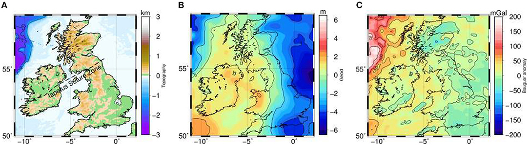
Figure 1. Geophysical observables used as constraining data sets. (A) ETOPO2v2 2-min gridded global relief data (National Geophysical Data Center, 2006). Iapetus Suture Zone is indicated by dashed line. (B) Geoid anomalies from XGM2016 global model (Pail et al., 2018). The geoid signal has been filtered to remove long wavelengths (>4,000 km, degrees 2–9) of mostly deep origin. Isolines every 2 m. (C) Bouguer anomaly map computed from free-air satellite data (XGM2016) corrected by FA2BOUG software (Fullea et al., 2008) with the onshore data from Great Britain Land Gravity Survey and from the Dublin Institute for Advanced Studies and the Geological Survey of Northern Ireland. Isolines every 50 mGal.
The geometry of the Moho discontinuity has been addressed in several studies in the area from a seismic perspective, mostly refraction/reflection profiles (Landes et al., 2005; Kelly et al., 2007) and receiver functions (e.g., Champion et al., 2006; Tomlinson et al., 2006; Davis et al., 2012; Licciardi et al., 2014, and references therein). Seismic ambient noise studies in Great Britain have imaged the crustal velocity structure with high resolution, showing considerable lateral heterogeneity (Nicolson et al., 2014; Galetti et al., 2017). Other crustal studies in the British Isles are based primarily on gravity data (e.g., Readman et al., 1997; Al-Kindi et al., 2003; Tiley et al., 2003).
Travel time body wave tomography models in Europe image positive velocity anomalies in central-southern England, Wales, and Scotland, and negative anomalies in the southern half of Ireland (e.g., Amaru, 2007). Surface wave tomography models at European scale are comparatively smoother. These models show as the most outstanding feature a clear N-S divide between slow Ireland and fast Great Britain in the upper mantle (e.g., Schivardi and Morelli, 2011; Legendre et al., 2012). A more recent adjoint waveform propagation tomography model in Europe exhibits fast upper mantle shear wave speeds in the eastern margins of Scotland and England and southwestern Irish margin, whereas slow upper mantle is restricted to the S-W English peninsula (Zhu et al., 2015). Local seismic p-wave tomography studies are characterized by relatively moderate lateral variations in the seismic velocities across Ireland, with positive lithospheric anomalies in the western area (e.g., Wawerzinek et al., 2008; O'Donnell et al., 2011). In Great Britain, a local Vp travel time tomography model suggests positive velocity anomalies in S-E England and S-E Scotland and negative anomalies in the Irish Sea, western Scotland, southern Wales margin and S-W English peninsula (Arrowsmith et al., 2005).
A seismic receiver functions study has suggested a significant thinning toward the north of Ireland related to the Iceland mantle plume (Landes et al., 2007). Fullea et al. (2014) also found a moderate lithospheric thinning in N-W Ireland using an integrated geophysical-petrological approach similar to the one used in this paper. These authors modeled a moderate lithospheric thickening in the western Irish margin aligned with the ISZ. More recently Root et al. (2017) have studied the mantle density structure of the British Isles and surrounding areas combining gravity data and seismic tomography models (e.g., Schaeffer and Lebedev, 2013) utilizing different crustal models: CRUST1.0 (Laske et al., 2013), EuCRUST-07 (Tesauro et al., 2008) and Kelly et al. (2007).
In this study, we use surface elevation, gravity and geoid anomalies, and gravity gradients as constraining data sets to infer the lithospheric structure in the British Isles (Figure 1). Elevation comes from ETOPO2v2 2-min gridded global relief data (National Geophysical Data Center, 2006). Geoid anomalies come from XGM2016 global Earth model (Pail et al., 2018). The geoid signal has been filtered to remove long wavelengths (>4,000 km, degrees 2–9) of mostly deep origin and retain the effects of lateral density variations shallower than ~400 km depth (e.g., Bowin, 2000). Bouguer anomalies were computed from free-air satellite data (XGM2016) corrected using the software FA2BOUG for a reduction density of 2,670 kg/m3 (Fullea et al., 2008). For the onshore Britain data from GB Land Gravity Survey was used (http://www.bgs.ac.uk/products/geophysics/landGravity.html), for onshore Ireland Bouguer anomalies were measured and corrected by the Dublin Institute for Advanced Studies and the Geological Survey of Northern Ireland (Readman et al., 1997, and references therein).
Gravity gradients (Figure 2) were taken from the recent global satellite-only gradiometric gravity model GOCO05S (http://www.goco.eu/, Mayer-Gürr et al., 2015) based on GOCE satellite data. The gradients are computed from degree 10 up to degree and order 220 (lateral resolution of about 90 km) at the satellite height (255 km) using a spherical harmonics synthesis code (see Appendix in Fullea et al., 2015; Martinec and Fullea, 2015). The GOCE gravity gradients are referred to the Local-North Oriented Frame (LNOF). LNOF is a right-handed local Cartesian system with its X axis pointing North, its Y axis pointing West, and its Z axis pointing radially outwards, defined with respect to spherical coordinates. Here we work in a Cartesian reference frame (MRF) using UTM projection and hence GOCO05S data are rotated from LNOF to MRF (x → E, y → N, z → up) following Bouman et al. (2013), and then used as input data in the models.
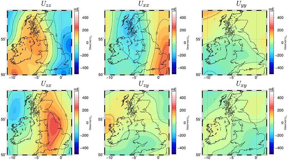
Figure 2. Geophysical observables used as constraining data sets. Observed gravity gradient components derived from the global gravity model GOCO05S based on GOCE satellite data. The gradients are computed using a spherical harmonic synthesis code from degree 10 up to 220 (see appendix in Fullea et al. (2015) and Martinec and Fullea (2015)). x-direction corresponds to E, y-direction to N and z-direction to vertical. Isolines every 100 mEötvös.
The main characteristics of the integrated geophysical-petrological approach used in this work (LitMod3D) are described elsewhere (Afonso et al., 2008; Fullea et al., 2009). Here we briefly summarize the main aspects relevant to the modeling purposes of this study.
In this paper, we adopt a definition of the lithosphere-asthenosphere boundary (LAB) based primarily on the temperature and compositional distributions. Therefore, we assume that the lithospheric mantle is defined: (1) thermally, as the portion of the mantle characterized by a conductive geotherm (i.e., its base is defined by a particular isotherm, see section below), and (2) compositionally, as the portion of the mantle characterized by a relatively depleted composition with respect to the fertile primary composition in the sub-lithosphere (i.e., PUM in Table 1).
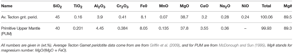
Table 1. Bulk mantle compositions used in this work from xenolith suites and peridotite massifs.
The lithospheric geotherm is computed in 3D under the assumption of steady-state heat conduction in the lithosphere, considering a P-T-dependent mantle thermal conductivity (Afonso et al., 2008; Fullea et al., 2009). As boundary conditions, we impose no lateral heat flow across the vertical limits of the model and fixed temperature at the surface (0°C) and at the base of the defined lithosphere (1,290°C). Heat production and thermal conductivity for each layer in our models are presented in Table 2. Between the lithosphere and sub-lithospheric mantle a “transition” region (buffer layer) with variable thickness and a continuous linear super-adiabatic gradient is assumed (i.e., heat transfer is controlled by both conduction and convection processes, see Fullea et al., 2009 for details). Below the buffer layer the geotherm is described by an adiabatic temperature gradient forced to be in the range 0.35–0.6 °C/km.
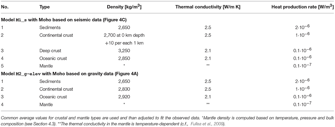
Table 2. Geophysical parameters in our preferred models.
Stable mineral assemblages in the mantle are calculated using a Gibbs free energy minimization scheme as described by Connolly (2005). The composition is defined within the major oxide system NCFMAS (Na2O-CaO-FeO-MgO-Al2O3-SiO2). All the stable assemblages in this study are based on the thermodynamic model and dataset presented in , Stixrude and Lithgow-Bertelloni (2005,2011). This approach allows for a self-consistent calculation of phase equilibria (identity and amount of mineral phases stable at a certain pressure and temperature) and physical properties. The density and seismic velocities in the mantle are determined according to the elastic moduli and density of each end-member mineral as described by Connolly and Kerrick (2002) and Afonso et al. (2008). In this study, we use the mantle compositions listed in Table 1.
A detailed description of the calculation of synthetic gravity and geoid anomalies and gravity gradients for a given 3D density distribution can be found in Fullea et al. (2009, 2014). The predicted/synthetic surface elevation in each model column (its buoyancy) is determined according to local isostasy by integrating the crustal and mantle densities from the surface down to the base of the model (400 km depth) and comparing subsequently with a calibration column (details on the calibration procedure are given in Afonso et al., 2008; Fullea et al., 2009).
For a modeling area of the considered size, magnetic anomalies need to be calculated within a spherical approach to account for possible edge and far-field effects (Baykiev et al., 2016). Here, we adopt an approach based on spherical prisms (tesseroids), with each having an uniform magnetization and susceptibility, to determine lithospheric magnetic anomalies (magnetic tesseroids software, Baykiev et al., 2016). The magnetic tesseroids are defined by the basement depth (top boundary) and the base of the magnetic crust (bottom boundary) given by the shallower of the either the petrological Moho or the Curie isotherm depth. Sediments are not considered here from a magnetic point of view as their magnetization and signal is usually low and related to short-wavelength anomalies out of the scope of this study. To avoid edge effects in the magnetic calculations, our models of British Isles are embedded into global models. The top and bottom surfaces of our modeling region, with edges at [N 50°; N 59°; E -11°; E 2°], are merged with the crystalline crust and Moho surfaces from CRUST1.0 model (Laske et al., 2013) by interpolation with an overlapping area of two degrees. The area outside of [N 48°; N 61°; E -13°; E 4°] is discretized with tesseroids of 1 degree longitudinal and latitudinal width, whereas inside our modeling area the tesseroids are 0.1 degrees in width. IGRF12 model (Thébault et al., 2015) with datum 2016-01-01 is used here as the inducing field to set magnetization vectors in each tesseroid across the model. The susceptibility distribution in our crustal model is derived from the VIS model of Hemant (2003) dividing by the thickness between the top and bottom magnetic boundaries in our model.
The models in our study consist of one sedimentary layer, two crustal layers (oceanic and continental) and one mantle layer (Table 2). For the sake of simplicity, we model a uniform lithospheric mantle with a single mantle composition (see Table 1). The latter implies that all the lateral variability in the mantle density distribution in our models will come from temperature variations only.
The sedimentary layer in our models is defined according to several datasets (Figure 3). The main source used to define the sedimentary layer is the North Atlantic compilation by Oakey and Stark, 1995. In the N-E corner of our study area (not covered by Oakey and Stark, 1995), data from the global data set by Whittaker et al. (2013) were used instead. In onshore Ireland, the geometry of the sediments was extracted from active seismic experiments (Landes et al., 2005, and references therein). Additionally, we used information from a seismic line across Great Britain (Barton, 1992), which was not included originally in the compilation by Oakey and Stark (1995).
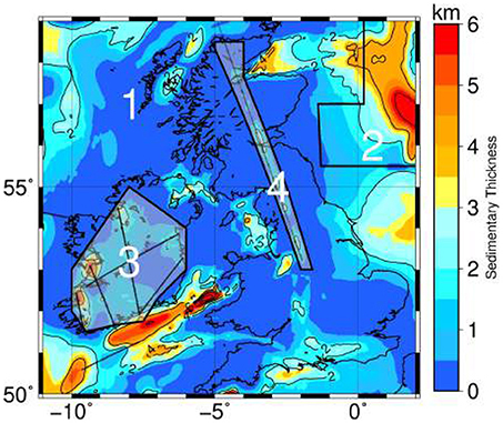
Figure 3. Combined model of sedimentary thickness. Dataset 1 corresponds to Oakey and Stark (1995), 2—Whittaker et al. (2013), 3—Landes et al. (2005), and 4—Barton (1992), see text for more details.
To define an initial model for the Moho and the base of the lithosphere (see Figures 4A,B) we carried out a 1D inversion of geoid anomaly and elevation data (Fullea et al., 2006, 2007). The 1D inversion method considers a simple two-layer lithospheric model (i.e., crust and lithospheric mantle) in which crustal density varies linearly with depth in order to accommodate pressure effects, whereas lithospheric mantle density is temperature-dependent only (i.e., neither compositional nor pressure effects are included). As a further refinement, the crystalline basement is defined as either oceanic or continental (see assigned properties in Table 2) essentially following bathymetric variations (Figures 1, 5). There are no lateral variations in the physical properties within each of the two crustal layers. As here we are only interested in the long wavelength lithospheric features we purposely exclude compositional/lithological details in the crust.
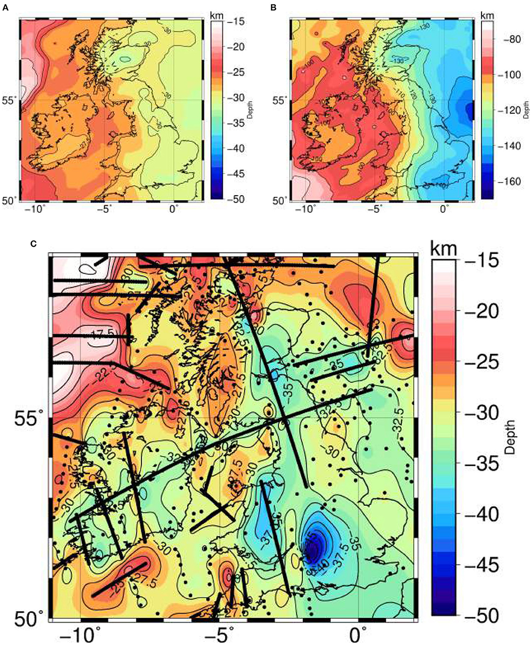
Figure 4. (A) Moho and (B) Lithosphere-Asthenosphere boundary according to 1D inversion of elevation and geoid anomalies (see text for more details). (C) Moho model derived from reflection, wide angle refraction and broad band and short period receiver function seismic data (Kelly et al., 2007; Davis et al., 2012; Licciardi et al., 2014, and references therein). The location of seismic data used to define the Moho surface is shown as black lines and dots.
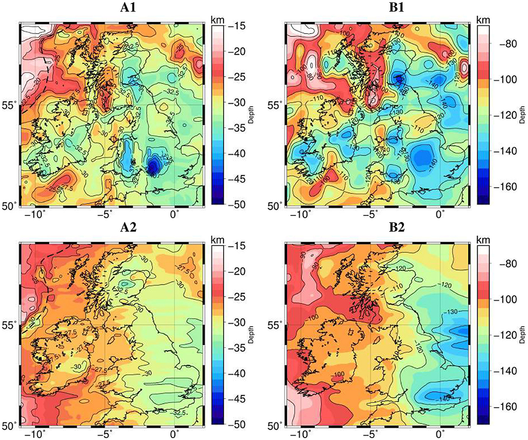
Figure 5. Moho and Lithosphere-Asthenosphere boundary of our end-member lithospheric models. (A) Moho depth. Isolines every 2.5 km. (B) Lithosphere-Asthenosphere boundary depth. Isolines every 10 km. First row corresponds to model M1_s (A1, B1), second row corresponds to model M2_g-elev (A2, B2). The dashed line in (A1,A2) indicates the boundary between oceanic and continental crustal domains.
The available crustal-scale seismic studies defining the geometry of the Moho discontinuity in our study region (see Section 2) have used different data sets covering different areas and that results in discrepancies in the models that can be locally relevant. Here we have generated a new seismically constrained Moho map based on all available seismic data. We use wide angle refraction and broadband and short period receiver function seismic data (Kelly et al., 2007; Davis et al., 2012; Licciardi et al., 2014, and references therein), and perform a smooth interpolation between data-points using Generic Mapping Tools (Wessel et al., 2013) program surface. The location of data points and the interpolated Moho surface is shown on the Figure 4C. Regarding the number of datapoints, our Moho model of the British Isles supersedes existing crustal models based on seismic data [e.g., CRUST1.0 (Laske et al., 2013), EuCRUST-07 (Kelly et al., 2007; Tesauro et al., 2008), EUNAseis, (Artemieva and Thybo, 2013)].
In this study we have defined two end-member models: (1) seismically derived Moho: M1_s; and (2) gravity-elevation derived Moho M2_g-elev. The rationale for this setting is to have the freedom to depart from the seismically constrained Moho during the modeling process in areas where matching other datasets is not possible modifying the other parameters within admissible bounds.
We modify the lithospheric geometry starting from our initial model to match the long wavelength gravity field and isostatic elevation based on trial and error forward modeling for both end-member crustal models: M1_s and M2_g-elev. For M2_g-elev we have also modified the initial crustal model as required whereas in the case of M1_s modifications were only allowed in areas without seismic constraints (Figure 4C, regions without seismic coverage). Model M2_g-elev can be regarded as a minimum structure, smooth model that matches gravity and local isostasy. In contrast, M1_s is a rougher model that includes apriori state-of-the-art seismic constraints on the geometry of both the Moho and the crystalline basement. In the case of M1_s we have incorporated a vertical crustal density gradient (i.e., pressure-dependent term) and an additional high-density layer at the bottom of the crust in areas of thick crust (>40 km) to realistically represent vertical density variations in the crust (e.g., southern Britain see Figure 5A1 and Table 2).
Our final lithospheric structure for M1_s and M2_g-elev is shown in Figure 5. The differences (residuals) between calculated and observed gravity and elevation data are shown in Figures 6, 7. The residuals for model M2_g-elev are due to small scale structures out of the scope in this study (e.g., granites in Ireland or in the SW English peninsula). For M1_s there are strong residuals in the Bouguer and geoid anomalies beneath Scotland and the Hebrides (labeled 1 and 2 in Figure 6). In the case of the gravity gradients, the residuals show the mismatch in the Hebrides but also in Wales and the Irish Sea. The interpretation of the gravity gradients is less straightforward than that for the gravity and geoid anomalies since for some gradient components the maximum sensitivity is not located directly below the causative density anomaly but shifted laterally (Martinec, 2014). For instance, the residual in the Irish Sea visible in Uzz and Uxx components is shifted toward S-E England in Uzx. Furthermore, the directional sensitivity in the gradients highlights the residual under the Irish Sea in the Uzz and the x (i.e., E-W) related components (Uxx and Uzx) but not in the y (i.e., N-S) related components. This suggests that the anomalous density structure beneath the Irish Sea is predominantly N-S oriented and hence visible in gradient components perpendicular to that trend. Our modeling results suggest that is not possible to reduce those anomalous high residuals without modifying the seismically derived Moho or adding lateral crustal density or mantle compositional variations. The second scenario is likely the case for the residual structures in the Irish Sea and Scotland although a further exploration of these features is out of the scope of this paper.

Figure 6. Difference between forward calculated and observed data (from Figure 1). (A) Elevation, (B) Geoid anomaly, (C) Bouguer anomaly. First row corresponds to model M1_s (A1–C1), second row corresponds to model M2_g-elev (A2–C2).
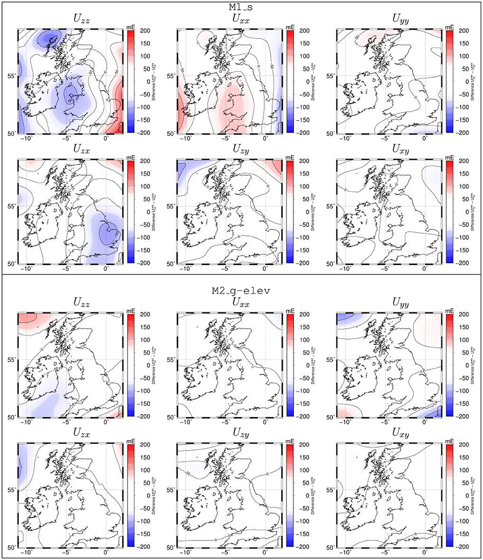
Figure 7. Difference between calculated and observed (Figure 2) gravity gradient tensor components at satellite level. Top panel corresponds to the model M1_s and bottom panel corresponds to model M2_g-elev.
The lithosphere changes considerably across our modeling domain in both M1_s and M2_g-elev. For model M2_g-elev there is a clear boundary roughly N-S trending dividing, to the west, an area of normal Phanerozoic crust and lithosphere (in Ireland, Wales, and NW Scotland) and, to the East, S-E Scotland and England where the lithosphere and crust are comparatively thicker (>100 and 30 km, respectively). This E-W division is still present in M1_s model but with considerably more short wavelength variations stemming from the crustal seismic a priori constraints included. The thickest crust and lithosphere in the two models are located in S-E Great Britain and in the N-E margin of England (>35 and 120 km, respectively). In contrast, the thinnest lithosphere is located beneath western Scotland, Northern Ireland, southern Irish margin and in the N-W oceanic domain.
Figure 8 shows the mantle density in M1_s model at different depths. The general pattern is dominated by dense material beneath S-E Great Britain and the British Atlantic margin, and a low-density anomaly in Scotland, Northern Ireland and the N-W offshore domain. This feature is also present in some of the models in the gravity-tomography study of Root et al. (2017). The lithospheric structure in Ireland in our M1_s model follows a pattern similar to that in Fullea et al. (2014), with a moderate thinning from S to N. Elastic thickness maps (derived from thermal and seismic data at European scale) reflecting the strength of the lithosphere are rather diverse in the British Isles (e.g., Cloetingh et al., 2005; Tesauro et al., 2009a,b). In spite of this fact, some common characteristics can be extracted: the elastic thickness tends to be higher in southern Great Britain and eastern Scotland and lower in Ireland, generally in line with our results.
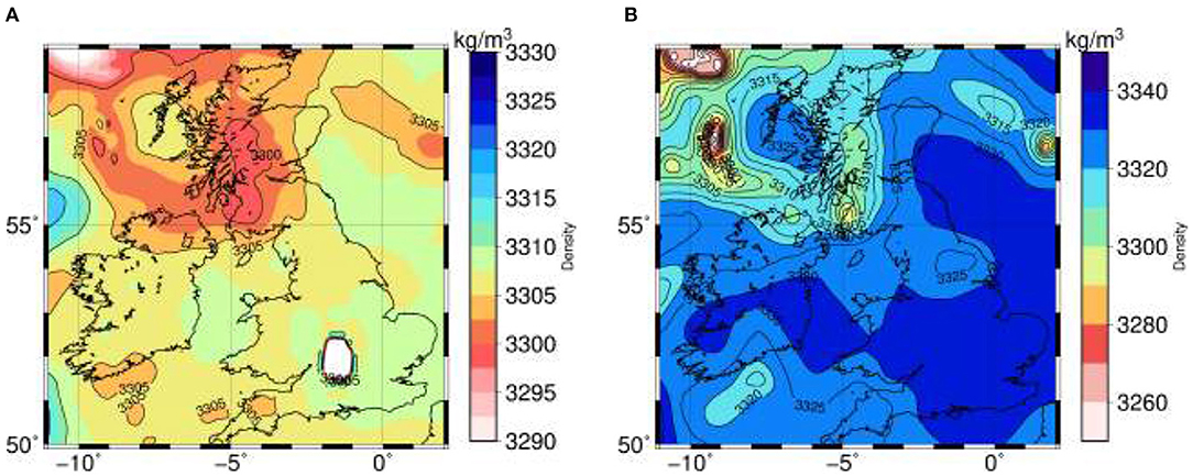
Figure 8. Calculated densities for model M1_s Figure 6. (A) Density at 42.5 km depth. Note that the white area in Great Britain corresponds to crustal material. (B) Density at 68.5 km depth.
Our end-member smooth model M2_g-elev is similar to surface wave tomography models (e.g., Schivardi and Morelli, 2011; Legendre et al., 2012) in that there is clear difference between Ireland and the western areas in Scotland and Wales (lithospheric thickness < 110 km), and Great Britain onshore and its eastern continental margin (lithospheric thickness >110 km). In the case of the end-member model with crustal seismic constraints (M1_s) the lithospheric architecture is more in agreement with local and regional p-wave and also adjoint waveform tomography images (e.g., Arrowsmith et al., 2005; Amaru, 2007; Wawerzinek et al., 2008; O'Donnell et al., 2011): thick, cold lithosphere beneath S-W Ireland, S-E Scotland and S-E England, and warm, relatively thin lithosphere in N-W Ireland and W Scotland.
Our predicted surface heat flow for model M1_s shows a rather flat pattern across the two islands with most of the values comprised in the range 55–65 mW/m2. This is partially in contrast with available borehole measurements: the amplitudes of the lateral variations are higher in some areas (e.g., across Great Britain) (Figure 9). Some of these discrepancies can be attributed to our simplified crustal model. For instance, we do not include igneous lithologies associated, in general, with high radiogenic heat production and therefore high surface heat flow (e.g., Leinster granite in Ireland or S-W English peninsula). Furthermore, we do not include lateral variations in crustal thermal properties (radiogenic heat production and thermal conductivity) in either the crystalline or the sedimentary layers that could affect the predicted heat flow locally. Other discrepancies could arise from near surface effects (e.g., water circulation) or lateral compositional variations in the lithospheric mantle not accounted for in this work. Shapiro and Ritzwoller (2004) computed an estimated global surface heat flow map based on a surface wave tomography model and a structural similarity statistical analysis. Their results are therefore similar to global tomography models, showing a clear boundary between Ireland and S-W Scotland on the one hand (heat flow values of 70–75 mW/m2), and Wales and England on the other hand (60–65 mW/m2). The predicted surface heat flow for model M1_s shows similar values in Wales and England but does not reproduce the increase of about 15 mW/m2 in Ireland and Scotland, with an increase of only approximately 5 mW/m2. Keeping in mind that the surface heat flow values derived by Shapiro and Ritzwoller (2004) are coming from a global tomography model, the discrepancies with our results here could be partially related to the lack of lateral chemical variations across the lithosphere in our models.
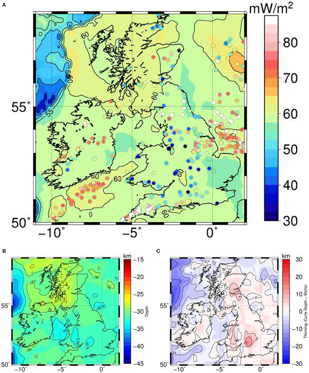
Figure 9. Thermal modeling results for model M1_s (see text for further details). (A) Synthetic surface heat flow. Dots show available measured heat flow data from the International Heat Flow Commission. (B) Synthetic Curie temperature depth. (C) Difference between Curie temperature and Moho depth. Red color represents areas where the Curie isotherm is above the Moho and vice versa.
M1_s model (Figure 5) is based on elevation, gravity and crustal seismic constraints. The associated 3D density distribution in the lithospheric mantle (Figure 8) is determined based on the temperature field (as the compositional field is constant throughout the whole model). The temperature is controlled by the lithospheric and crustal thickness and the thermal parameters (Table 2). Our 3D temperature modeling also predicts theoretical values for the depth of the Curie temperature, which would correspond to the lower boundary of possible magnetization in the lithosphere. Assuming a Curie temperature of 585°C (corresponding to magnetite), the base of the magnetic crust in M1_s model is shown in Figures 9B, 12A. Differences between the Curie depth and the Moho depth in the model are shown on the Figure 9C.
In M1_s model the predicted Curie temperature depth is shallower than the Moho in some areas, especially onshore. In these locations, the lowermost part of the crust (i.e., hotter than Curie temperature) is not contributing to the crustal magnetic field. Conversely, our predicted Curie isotherm is within the uppermost mantle in some areas (e.g., N-W marine domain). In the later case we take the seismic/petrological Moho as the effective lower magnetic boundary. The rationale for this is that the signal produced by possible sources in the upper mantle is rather weak when compared to crustal sources considering susceptibility values similar to those experimentally derived by Ferré et al. (2013) for mantle rocks (Baykiev et al., 2018).
In line with the exploratory purposes of this paper we consider a simplified crustal VIS model based on the work of Hemant (2003) and calculate the magnetic field at 5 km altitude, i.e., airborne level (Figure 10). In this way, our forward calculated synthetic crustal magnetic field represents the signal related to the geological units according to Hemant (2003) model and our lithospheric model (i.e., temperature and geometry of the crystalline basement). Since the model of Hemant (2003) is based on a global scale regionalization adjusted to match satellite magnetic data, our synthetic crustal magnetic field can only capture the most prominent induced anomalies of airborne, ship and satellite magnetic data, e.g., from EMAG2 model (Maus, 2009): anomalies in Scotland, N-W Wales or S-E England peninsula (Figure 10). Elsewhere, EMAG2 shows anomalies with amplitudes significantly higher than those in our synthetic field. This is related to small scale variations in the magnetic structure of the crust (i.e., lateral variations in susceptibility and remanence) not reflected in our simplified, first order model.
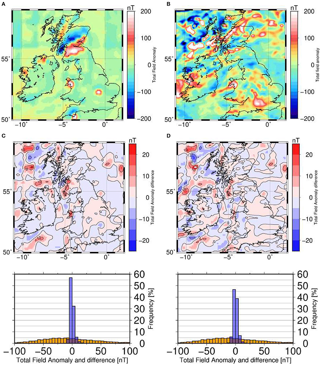
Figure 10. Forward calculated synthetic crustal magnetic field. (A) Forward calculated magnetic field anomaly associated with model M1_s assuming the vertical integrated susceptibility (VIS) derived from Hemant (2003). (B) EMAG-2 V2 Magnetic Anomaly (Maus, 2009). (C) Difference between the calculated magnetic anomaly for model M1_s (A in this figure) and for a flat model (30 km constant Curie depth) with VIS from Hemant (2003). Underneath: histogram of values in EMAG2 dataset (orange) and in this difference map (blue) (D) Difference between the calculated magnetic anomaly for model M1_s (A) and for model M2_g-elev with VIS from Hemant (2003). Underneath: histogram of values in EMAG2 dataset (orange) and in the difference map (blue).
The main goal of our magnetic modeling exercise is to quantify the effect of the lithospheric structure (thermal field) in the synthetic crustal magnetic field. The vertically integrated susceptibility model of Hemant (2003) reflects the magnetic properties of the entire magnetic column, i.e., VIS is susceptibility multiplied by thickness. Hemant (2003) VIS model is based on data at satellite altitude where the signal caused by variations in magnetic thickness are negligible in our study region. However, at the airborne altitude, magnetic thickness has a non-negligible signal.
To better illustrate this point we calculate the differences between the magnetic field of M1_s model (with lateral Curie depth variations) and a flat model (30 km constant Curie depth) for the same VIS model (i.e., Hemant, 2003) and the same top magnetic boundary (i.e., basement geometry). Note that susceptibilities in these models are not identical, only the susceptibility multiplied by the magnetic thickness (which corresponds to the total VIS). The effect of accounting for thickness variations translates into magnetic field differences of up to 23 nT with comparatively longer wavelengths than the airborne/satellite/ship data. To further assess the temperature related effect, we make a new comparison, now between our end-member models M1_s and M2_g-elev for the same VIS: the differences are slightly larger in amplitude in this case (up to 28 nT) and the spatial pattern shows comparatively higher frequencies (Figure 10).
The comparison between different temperature lithospheric models assuming constant VIS values is a conservative estimate of the thermal related magnetic effect. Another option to quantify the effect of the lithospheric structure in the magnetic field is to consider fixed susceptibilities instead of VIS. In that case, an increase (or decrease) in crustal temperature would decrease (or increase) the thickness of the magnetic layer due to depth variations in the Curie temperature.
To evaluate the full thermal effect we consider the susceptibility distribution from M1_s VIS model and combine it with the geometry from M2_g-elev and two flat models (30 and 40 km constant Curie depth). The 30-km-flat model is close to the average Curie temperature depth for M1_s whereas the 40-km-flat model represents a much thicker (or colder) model comparatively. The tests, in this case, show stronger effects in the synthetic signal going up to 84 nT for the differences with respect to the 30-km-flat model and 63 nT for the differences with respect to M2_g-elev (see Figure 11). The maximum differences for M1_s are up to 367 nT with respect to the 40-km-flat model.
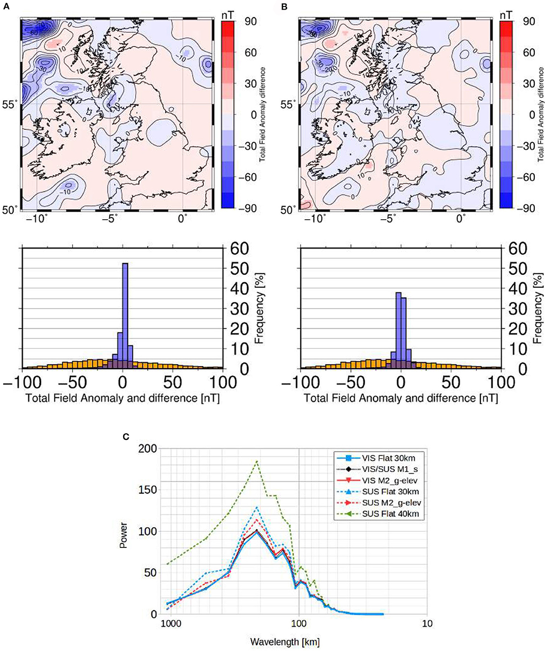
Figure 11. (A) Difference between the calculated magnetic anomaly for model M1_s (Figure 10A) and for a flat model (30 km constant Curie depth) with the same susceptibility distribution as in M1_s. Below: histogram of values in EMAG2 dataset (orange) and in this difference map (blue) (B) Difference between the calculated magnetic anomaly for model M1_s (Figure 10A) and for model M2_g-elev with the same susceptibility distribution as in M1_s. Underneath: histogram of values in EMAG2 dataset (orange) and in the difference map (blue). (C) Estimated power spectrums in the radial direction of five magnetic models, where VIS means models with VIS from Hemant (2003), and SUS means models with susceptibility distribution from M1_s.
Most of the magnetic anomalies in EMAG-2 in our study region are within ± 100 nT range, with a standard deviation of 66.1 nT. Assuming constant VIS, in the case of the differences between M1_s and the 30-km-flat model the standard deviation is 3.34 nT (5% of EMAG-2 standard deviation), whereas in the case of the differences between models M1_s and M2_g-elev the standard deviation is 3.76 nT (6% of EMAG-2 standard deviation) (histograms in Figure 10). In the scenario where susceptibility is kept fixed (Figure 11), the standard deviation for the difference between M1_s and the 30-km-flat and 40-km-flat model is 9.6 and 45.4 nT, respectively (15 and 68.7% of EMAG-2 standard deviation, respectively), and for the difference between M1_s and M2_g-elev it is 7 nT (11%). Therefore, the effect related to typical variations in the magnetic boundary geometry (i.e., Curie temperature) represents on average 5-15% of the total magnetic signal at airborne level. In the case of strong temperature/magnetic boundary variations, this effect rises up to almost 70%.
The radial power spectrum of the magnetic models computed for a constant VIS is very similar whereas the models computed using a fixed susceptibility are considerably different (Figure 11C). The magnetic thickness variations in the case of models with constant VIS induce magnetic field anomalies mostly in the horizontal components (north and east). In contrast, magnetic thickness variations assuming a fixed susceptibility distribution predominantly modify the vertical, z-component of the induced signal, which is larger in amplitude with respect to the horizontal components. The spectral amplitude differences with respect to M1_s in the case of fixed susceptibility are relatively modest and concentrated around wavelengths of 200 km for models M2_g-elev and 30-km-flat (Figure 11C). However, in the case of the 40-km-flat model there is a significant increase in the spectral amplitude starting from wavelengths > 70 km.
As stated before, the Curie temperature depth in our models depends on the lithospheric structure constrained by gravity field, elevation and seismic data, and thermal parameters (thermal conductivity and heat production rate). Szwillus et al. (submitted) presented a Curie temperature depth model based on global surface heat flow data (Davies, 2013), seismological structure [LITHO1.0 model Pasyanos et al. (2014), CRUST1.0 model for the crustal thickness Laske et al. (2013)] and oceanic floor age (Müller et al., 2008). These authors inverted in 1D the heat flow value considering the 1D conduction equation over continental areas (for the assumed lithospheric model) and the half-space thermal cooling model for oceanic areas (Figure 12B). The Curie temperature map of Szwillus et al. (submitted) agrees with the 3D temperature from our M1_s model in some large-scale lateral features (e.g., shallow Curie depth under Scotland, cold crust in S-E Great Britain). However, differences between the two methods are apparent, in particular in the amplitude of the lateral temperature variations (e.g., offshore, southern Irish margin or northeastern English margin). The method used in Szwillus et al. (submitted) relies on surface heat flow measurements which are in general sparse, especially in oceanic areas and often affected by near-surface effects not necessarily related to the magnetic structure. A direct translation of the temperatures in Szwillus et al. (submitted) would likely lead to density values that would predict relatively large gravity field anomalies for the assumed fixed lithospheric geometry (CRUST1.0, LITHO1.0). Our approach in this study is not based on the observed surface heat flow measurements although such constraint can be naturally incorporated into the work-flow as our model does predict synthetic surface heat flow values. Instead, our models are primarily constrained by gravity field and elevation data, available everywhere in our model with regular resolution, with additional constraints from state-of-the-art seismic data in the crust. Furthermore, the thermal problem is solved in 3D in our scheme, allowing therefore to model a comparatively more complex lithospheric structure. As stated in the previous section, appropriate modeling of surface heat flow measurements should include lateral variations in thermal crustal properties, a feature that is not included in this work.
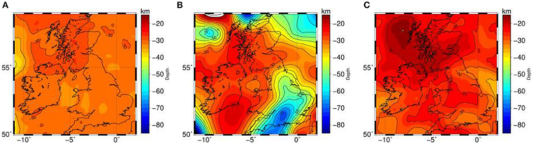
Figure 12. Curie temperature depth maps. (A) Curie temperature depth from model M_1-s. (B) Curie temperature depth estimated from surface heat flow by Szwillus et al. (submitted). Reproduced from Szwillus et al. (submitted) by the permission of copyright holder [Szwillus W.]. (C) Curie temperature depth estimated from EMAG2. Reproduced from Li et al. (2017) by the permission of copyright holder [Li C.-F.].
The work of Li et al. (2011) focused on the North Atlantic area, used a spectral approach to derive Curie temperature depths: inversion of magnetic anomalies with a fractal magnetization model. In a recent paper Li et al., 2017 used the same approach at the global scale to derive Curie temperature depths from magnetic anomalies (EMAG2) using window sizes of 49.4, 97.5, and 98.8 km for their calculations. Some of the features in Li et al. (2017) model (Figure 12C) are consistent with the thermal predictions based on our models (and also with the results by Szwillus et al., submitted): high temperature-shallow Curie isotherm between Scotland and Northern Ireland (North Atlantic Igneous Province) and cold temperature-deep Curie isotherm south of Great Britain and in the eastern English margin. There are, however, significant discrepancies in other areas (e.g, the Irish Sea, England or the Hebrides). Some of this differences could be related to misinterpretation of short-wavelength anomalies (e.g., west of the Hebrides) in terms of thermal variations. As suggested by our results, excluding areas with strong temperature gradients, in general only 5–15 % of the crustal magnetic signal at airborne level stems from lateral temperature variations (Figure 10) with susceptibility and remanence lateral variations contributing the remaining 85–95%.
Our synthetic tests to assess the effect of laterally varying Curie depth show that if the VIS distribution is kept constant, geometrical variations in the magnetic thickness produce a non-negligible anomaly signal while the power spectrum remains almost unaltered. Tests with fixed susceptibility and varying Curie depth show comparatively larger synthetic magnetic anomalies and associated changes in the spectrum. Our results indicate that significant lateral temperature variations (e.g., difference between M1_s and 40-km-flat model) that translate into conspicuous variations in the magnetic signal power spectrum (Figure 11C) could likely be identified by Curie depth spectral estimation techniques, depending on the spatial window size and the range of matched wavelengths used. However, typical lateral thermal field variations (as exemplified by the differences between M1_s and 30-km-flat model or between M1_s and M2_g-elev) are associated with relatively minor changes in the power spectra and, hence, would remain hardly detectable for spectral-based techniques.
The question of the magnetic contribution from the lithospheric mantle is under discussion (e.g., Ferré et al., 2013). In any case, the contribution from the uppermost mantle seems to be considerably weaker than the crustal one (Baykiev et al., 2018). If in the area of study the Curie isotherm is located beneath the Moho and there is no magnetic mantle material or the mantle magnetic susceptibility is very low, spectral methods would not be able to estimate the Curie depth correctly; instead, spectral methods would find the effective magnetic thickness, in this case the petrological Moho depth. This shows the importance of carrying out lithospheric modeling by other means in order to characterize the thermal field and the Curie isotherm depth.
In this paper, we use a methodology (LitMod3D) that allows for forward modeling of the Curie temperature depth based on seismic, elevation and gravity observations within an integrated geophysical-petrological approach. We solve the 3D heat conduction problem and determine the density in the mantle self-consistently based on temperature, pressure, and bulk composition. Here, we couple, via Curie temperature depth, the thermal output from LitMod with a spherical magnetic modeling software (Baykiev et al., 2016) in order to compute synthetic crustal magnetic anomalies.
We have tested our approach in the British Isles and surrounding areas. Our best fitting end-member models M1_s and M2_g-elev are able to reproduce the long-wavelength component of the gravity field and surface elevation (Figure 6). The crust and lithospheric thicknesses are characterized by lateral variations across the model domain, with Great Britain being characterized in general by thicker and colder lithosphere, especially in the south-east. The thinnest and warmest lithosphere is located beneath west Scotland, Northern Ireland and in the N-W oceanic area. Our smooth model M2_g-elev exhibits lower misfits than the end-member model that integrates a new state-of-the-art crystalline basement and Moho geometry model based on all available seismic data, M1_s. In the latter case (M1_s) the most conspicuous misfits are likely related to an oversimplified crustal model with only very broad lateral variations in physical properties and perhaps inaccuracies/inconsistencies in the seismic crustal models. While the simplifications assumed in the lithospheric structure here are appropriate for the exploratory purposes of this paper, our future work will involve integrated lithospheric modeling including seismic tomography, surface heat flow and petrological data sets (to constrain the mantle chemical structure) as well as small-scale lithological features, including a fully consistent petrological crustal metastable model.
Our best fitting models predicts a map of the depth of the Curie isotherm capturing some long wavelength characteristics of Curie temperature models inverted from magnetic anomalies or global heat flow and seismic tomography models: high temperature-shallow Curie isotherm between Scotland and Northern Ireland (North Atlantic Igneous Province) and cold temperature-deep Curie isotherm south of Great Britain and in the eastern English margin. However, differences elsewhere and in the amplitude of the temperature variations are apparent among all three approaches.
We have calculated a synthetic crustal magnetic field at 5 km altitude, i.e., airborne level, based on our lithospheric thermal model and a simplified crustal susceptibility model derived from Hemant (2003), and estimated the relative weight of typical lateral variations in the Curie isotherm depth in observed crustal magnetic anomalies: 5–15 % with localized areas of > 70%. Therefore, typical variations in the assumed Curie temperature depth in our study region have a considerable effect on the magnetic signal although that is not clearly visible in their power spectra. This highlights the importance of a precise characterization of the Curie isotherm topography for magnetic modeling using additional complementary constraints as illustrated in this work.
In spite of capturing a few of the main anomalies visible in EMAG-2 model based on airborne/satellite/ship data, most of the synthetic magnetic signal based in our lithospheric models is not matching the observed anomalies. This is not surprising given the relative simplicity of our crustal magnetic model. This misfit along with the fact that some of the short wavelength features inferred in magnetically derived thermal models seem to be artifacts related to remanence or lateral variations in susceptibility points us to our next step: forward model and inversion of airborne and satellite magnetic anomalies for lateral susceptibility (and possibly remanence) variations in the crust using as background an improved thermal model based on gravity, elevation, and seismic data as discussed here.
EB performed the forward modeling, implemented programs to couple LitMod3D and magnetic tesseroids, wrote the original manuscript and made all figures. MG worked on modifications in LitMod3D for thermal calculations and performed thermal calculations. JF helped with LitMod3D, contributed with ideas and assistance, made a major revision of the manuscript and wrote parts of it.
EB and MG have received funding from Science Foundation Ireland grant iTHERC (16/ERCD/4303) to JF.
The authors declare that the research was conducted in the absence of any commercial or financial relationships that could be construed as a potential conflict of interest.
All figures were made using the Generic Mapping Tools (Wessel et al., 2013). We want to thanks Richard England, Nicky White, and Andrea Licciardi for providing the seismic data that was used to create the Moho model.
Afonso, J. C., Fernàndez, M., Ranalli, G., Griffin, W. L., and Connolly, J. A. D. (2008). Integrated geophysical-petrological modeling of the lithosphere and sublithospheric upper mantle: Methodology and applications. Geochem. Geophys. Geosyst. 9. doi: 10.1029/2007GC001834
Al-Kindi, S., White, N., Sinha, M., England, R., and Tiley, R. (2003). Crustal trace of a hot convective sheet. Geology 31, 207–210. doi: 10.1130/0091-7613(2003)031<0207:CTOAHC>2.0.CO;2
Álvarez, O., Gimenez, M., Folguera, A., Spagnotto, S., Bustos, E., Baez, W., et al. (2015). New evidence about the subduction of the copiapó ridge beneath South America, and its connection with the chilean-pampean flat slab, tracked by satellite GOCE and EGM2008 models. J. Geodyn. 91, 65–88. doi: 10.1016/j.jog.2015.08.002
Amaru, M. L. (2007). Global Travel Time Tomography with 3-D Reference Models. Ph.D. thesis, Utrecht University.
Arrowsmith, S. J., Kendall, M., White, N., VanDecar, J. C., and Booth, D. C. (2005). Seismic imaging of a hot upwelling beneath the British Isles. Geology 33:345. doi: 10.1130/G21209.1
Artemieva, I. M., and Thybo, H. (2013). EUNAseis: A seismic model for Moho and crustal structure in Europe, Greenland, and the North Atlantic region. Tectonophysics 609, 97–153. doi: 10.1016/j.tecto.2013.08.004
Barton, P. J. (1992). LISPB revisited: a new look under the Caledonides of Northern Britain. Geophys. J. Int. 110, 371–391. doi: 10.1111/j.1365-246X.1992.tb00881.x
Baykiev, E., Ebbing, J., Brönner, M., and Fabian, K. (2016). Forward modeling magnetic fields of induced and remanent magnetization in the lithosphere using tesseroids. Comput. Geosci. 96, 124–135. doi: 10.1016/j.cageo.2016.08.004
Baykiev, E., Ebbing, J., Brönner, M., and Fabian, K. (2018). Spherical magnetic field gradients and lithospheric magnetization (part 1) : finite difference calculation and depth sensitivity to lithospheric magnetization. Geophys. J. Int. 215, 1747–1765. doi: 10.1093/gji/ggy363
Bouman, J., Ebbing, J., and Fuchs, M. (2013). Reference frame transformation of satellite gravity gradients and topographic mass reduction. J. Geophys. Res. Solid Earth 118, 759–774. doi: 10.1029/2012JB009747
Bowin, C. (2000). Mass anomaly structure of the Earth. Rev. Geophys. 38, 355–387. doi: 10.1029/1999RG000064
Champion, M. E. S., White, N. J., Jones, S. M., and Priestley, K. F. (2006). Crustal velocity structure of the British Isles; a comparison of receiver functions and wide-angle seismic data. Geophys. J. Int. 166, 795–813. doi: 10.1111/j.1365-246X.2006.03050.x
Chappell, A. R., and Kusznir, N. J. (2008). Three-dimensional gravity inversion for Moho depth at rifted continental margins incorporating a lithosphere thermal gravity anomaly correction. Geophys. J. Int. 174, 1–13. doi: 10.1111/j.1365-246X.2008.03803.x
Chew, D. M., and Stillman, C. J. (2009). “Late Caledonian Orogeny and magmatism,” in The Geology of Ireland, 2nd edn., eds C. H. Holland and I. S. Sanders (Edinburg: Dunedin Academic Press), 143–173.
Cloetingh, S., Ziegler, P., Beekman, F., Andriessen, P., Matenco, L., Bada, G., et al. (2005). Lithospheric memory, state of stress and rheology: neotectonic controls on Europe's intraplate continental topography. Q. Sci. Rev. 24, 241–304. doi: 10.1016/j.quascirev.2004.06.015
Connolly, J. (2005). Computation of phase equilibria by linear programming: A tool for geodynamic modeling and its application to subduction zone decarbonation. Earth Planet. Sci. Lett. 236, 524–541. doi: 10.1016/j.epsl.2005.04.033
Connolly, J., and Kerrick, D. (2002). Metamorphic controls on seismic velocity of subducted oceanic crust at 100–250 km depth. Earth Planet. Sci. Lett. 204, 61–74. doi: 10.1016/S0012-821X(02)00957-3
Davies, J. H. (2013). Global map of solid Earth surface heat flow. Geochem. Geophy. Geosyst. 14, 4608–4622. doi: 10.1002/ggge.20271
Davis, M. W., White, N. J., Priestley, K. F., Baptie, B. J., and Tilmann, F. J. (2012). Crustal structure of the British Isles and its epeirogenic consequences. Geophys. J. Int. 190, 705–725. doi: 10.1111/j.1365-246X.2012.05485.x
Ebbing, J., Bouman, J., Fuchs, M., Gradmann, S., and Haagmans, R. (2014). “Sensitivity of goce gravity gradients to crustal thickness and density variations: case study for the northeast atlantic region,” in Gravity, Geoid and Height Systems, ed U. Marti (Cham: Springer International Publishing), 291–298.
Ebbing, J., Bouman, J., Fuchs, M., Verena, L., Haagmans, R., Meekes, J. A. C., et al. (2013). Advancements in satellite gravity gradient data for crustal studies. Leading Edge 32, 900–906. doi: 10.1190/tle32080900.1
Ebbing, J., Braitenberg, C., and Götze, H.-J. (2006). The lithospheric density structure of the Eastern Alps. Tectonophysics 414, 145–155. doi: 10.1016/j.tecto.2005.10.015
Ferré, E. C., Friedman, S. A., Martín-Hernández, F., Feinberg, J. M., Conder, J. A., and Ionov, D. A. (2013). The magnetism of mantle xenoliths and potential implications for sub-Moho magnetic sources. Geophys. Res. Lett. 40, 105–110. doi: 10.1029/2012GL054100
Fullea, J., Afonso, J. C., Connolly, J. A. D., Fernàndez, M., García-Castellanos, D., and Zeyen, H. (2009). LitMod3D: An interactive 3-D software to model the thermal, compositional, density, seismological, and rheological structure of the lithosphere and sublithospheric upper mantle. Geochem. Geophys. Geosyst. 10. doi: 10.1029/2009GC002391
Fullea, J., Fernàndez, M., and Zeyen, H. (2006). Lithospheric structure in the Atlantic–Mediterranean transition zone (Southern Spain, Northern Morocco): a simple approach from regional elevation and geoid data. Comptes Rendus Geosci. 338, 140–151. doi: 10.1016/j.crte.2005.11.004
Fullea, J., Fernàndez, M., and Zeyen, H. (2008). FA2BOUG—A FORTRAN 90 code to compute Bouguer gravity anomalies from gridded free-air anomalies: Application to the Atlantic-Mediterranean transition zone. Comput. Geosci. 34, 1665–1681. doi: 10.1016/j.cageo.2008.02.018
Fullea, J., Fernàndez, M., Zeyen, H., and Vergés, J. (2007). A rapid method to map the crustal and lithospheric thickness using elevation, geoid anomaly and thermal analysis. Application to the Gibraltar Arc System, Atlas Mountains and adjacent zones. Tectonophysics 430, 97–117. doi: 10.1016/j.tecto.2006.11.003
Fullea, J., Muller, M., Jones, A., and Afonso, J. (2014). The lithosphere–asthenosphere system beneath Ireland from integrated geophysical-petrological modeling II: 3D thermal and compositional structure. Lithos 189, 49–64. doi: 10.1016/j.lithos.2013.09.014
Fullea, J., Rodríguez-González, J., Charco, M., Martinec, Z., Negredo, A., and Villaseñor, A. (2015). Perturbing effects of sub-lithospheric mass anomalies in GOCE gravity gradient and other gravity data modelling: Application to the Atlantic-Mediterranean transition zone. Int. J. Appl. Earth Observ. Geoinform. 35, 54–69. doi: 10.1016/j.jag.2014.02.003
Galetti, E., Curtis, A., Baptie, B., Jenkins, D., and Nicolson, H. (2017). Transdimensional Love-wave tomography of the British Isles and shear-velocity structure of the East Irish Sea Basin from ambient-noise interferometry. Geophys. J. Int. 208, 36–58. doi: 10.1093/gji/ggw286
Götze, H., Lahmeyer, B., Schmidt, S., and Strunk, S. (1994). “The lithospheric structure of the Central Andes (20–26°S) as inferred from interpretation of regional gravity,” in Tectonics of the Southern Central Andes, eds K. J. Reutter, E. Scheuber, and P. J. Wigger (Berlin; Heidelberg: Springer-Verlag GmbH), 7–21. doi: 10.1007/978-3-642-77353-2_1
Griffin, W. L., O'Reilly, S. Y., Afonso, J. C., and Begg, G. C. (2009). The composition and evolution of lithospheric mantle: a re-evaluation and its tectonic implications. J. Petrol. 50, 1185–1204. doi: 10.1093/petrology/egn033
Hahn, A., Ahrendt, H., Meyer, J., and Hufen, J. H. (1984). A model of magnetic sources within the earth's crust compatible with the field measured by the satellite MAGSAT. Geologisches Jahrbuch A75, 125–156.
Hemant, K. (2003). Modelling and Interpretation of Global Lithospheric Magnetic Anomalies. Scientific technical report, Deutsches GeoForschungsZentrum. Available online at: http://gfzpublic.gfz-potsdam.de/pubman/item/escidoc:8616:5/component/escidoc:8615/0310.pdf?mode=download
Hemant, K., and Maus, S. (2005). Geological modeling of the new CHAMP magnetic anomaly maps using a geographical information system technique. J. Geophys. Res. Solid Earth 110:B12103. doi: 10.1029/2005JB003837
Hinze, W. J., von Frese, R. R. B., and Saad, A. H. (2013). Gravity and Magnetic Exploration: Principles, Practices, and Applications. Cambridge: Cambridge University Press. doi: 10.1017/CBO9780511843129
Kaban, M. K., Schwintzer, P., and Tikhotsky, S. A. (1999). A global isostatic gravity model of the Earth. Geophys. J. Int. 136, 519–536. doi: 10.1046/j.1365-246x.1999.00731.x
Kelly, A., England, R. W., and Maguire, P. K. H. (2007). A crustal seismic velocity model for the UK, Ireland and surrounding seas. Geophys. J. Int. 171, 1172–1184. doi: 10.1111/j.1365-246X.2007.03569.x
Khan, A., Connolly, J. A. D., Maclennan, J., and Mosegaard, K. (2007). Joint inversion of seismic and gravity data for lunar composition and thermal state. Geophys. J. Int. 168, 243–258. doi: 10.1111/j.1365-246X.2006.03200.x
Landes, M., Ritter, J., and Readman, P. (2007). Proto-Iceland plume caused thinning of Irish lithosphere. Earth Planet. Sci. Lett. 255, 32–40. doi: 10.1016/j.epsl.2006.12.003
Landes, M., Ritter, J. R. R., Readman, P. W., and O'Reilly, B. M. (2005). A review of the Irish crustal structure and signatures from the Caledonian and Variscan Orogenies. Terra Nova 17, 111–120. doi: 10.1111/j.1365-3121.2004.00590.x
Laske, G., Masters, G, Ma, Z., and Pasyanos, M. (2013). Update on CRUST1.0 - A 1-degree Global Model of Earth's Crust. Poster on EGU General Assembly 2013 (Vienna).
Legendre, C. P., Meier, T., Lebedev, S., Friederich, W., and Viereck-Götte, L. (2012). A shear wave velocity model of the European upper mantle from automated inversion of seismic shear and surface waveforms. Geophys. J. Int. 191, 282–304. doi: 10.1111/j.1365-246X.2012.05613.x
Li, C.-F., Lu, Y., and Wang, J. (2017). A global reference model of Curie-point depths based on EMAG2. Sci. Rep. 7:45129. doi: 10.1038/srep45129
Li, C.-F., Wang, J., Lin, J., and Wang, T. (2013). Thermal evolution of the North Atlantic lithosphere: New constraints from magnetic anomaly inversion with a fractal magnetization model. Geochem. Geophys. Geosyst. 14, 5078–5105. doi: 10.1002/2013GC004896
Li, Z., Hao, T., Xu, Y., and Xu, Y. (2011). An efficient and adaptive approach for modeling gravity effects in spherical coordinates. J. Appl. Geophys. 73, 221–231. doi: 10.1016/j.jappgeo.2011.01.004
Licciardi, A., Agostinetti, N. P., Lebedev, S., Schaeffer, A. J., Readman, P. W., and Horan, C. (2014). Moho depth and VP/VS in Ireland from teleseismic receiver functions analysis. Geophys. J. Int. 199, 561–579. doi: 10.1093/gji/ggu277
Martinec, Z. (2014). Mass-density Green's functions for the gravitational gradient tensor at different heights. Geophys. J. Int. 196, 1455–1465. doi: 10.1093/gji/ggt495
Martinec, Z., and Fullea, J. (2015). A refined model of sedimentary rock cover in the southeastern part of the Congo basin from goce gravity and vertical gravity gradient observations. Int. J. Appl. Earth Observ. Geoinform. 35, 70–87. doi: 10.1016/j.jag.2014.03.001
Martos, Y. M., Catalán, M., Jordan, T. A., Golynsky, A., Golynsky, D., Eagles, G., et al. (2017). Heat flux distribution of Antarctica unveiled. Geophys. Res. Lett. 44, 11417–11426. doi: 10.1002/2017GL075609
Masterton, S. M., Gubbins, D., Müller, R. D., and Singh, K. H. (2012). Forward modelling of oceanic lithospheric magnetization. Geophys. J. Int. 192, 951–962. doi: 10.1093/gji/ggs063
Maule, C. F., Purucker, M. E., Olsen, N., and Mosegaard, K. (2005). Heat flux anomalies in Antarctica revealed by satellite magnetic data. Science 309, 464–467. doi: 10.1126/science.1106888
Maus, S. (2009). Emag2: Earth Magnetic Anomaly Grid (2-Arc-Minute Resolution). National Centers for Environmental Information, NOAA.
Maus, S. (2010). Magnetic Field Model MF7. Available online at: https://geomag.us/models/MF7.html
Mayer-Gürr, T., Kvas, A., Klinger, B., Rieser, D., Zehentner, N., Pail, R., et al. (2015). “The new combined satellite only model GOCO05s,” in Conference: EGU General Assembly 2015 (Vienna).
Maystrenko, Y. P., and Scheck-Wenderoth, M. (2013). 3D lithosphere-scale density model of the Central European Basin system and adjacent areas. Tectonophysics 601, 53–77. doi: 10.1016/j.tecto.2013.04.023
McDonough, W., and Sun, S.-S. (1995). The composition of the Earth. Chem. Geol. 120, 223–253. doi: 10.1016/0009-2541(94)00140-4
Meyer, J., Hufen, J.-H., Siebert, M., and Hahn, A. (1983). Investigations of the internal geomagnetic field by means of a global model of the Earth's crust. J. Geophy. 52, 71–84.
Müller, R. D., Sdrolias, M., Gaina, C., and Roest, W. R. (2008). Age, spreading rates, and spreading asymmetry of the world's ocean crust. Geochem. Geophys. Geosys. 9. doi: 10.1029/2007GC001743
National Geophysical Data Center (2006). 2-Minute Gridded Global Relief Data (Etopo2) v2. Available online at: https://www.ngdc.noaa.gov/mgg/global/etopo2.html; https://data.noaa.gov//docucomp/page?xml=NOAA/NESDIS/NGDC/MGG/DEM/iso/xml/301.xml&view=getDataView&header=none
Nicolson, H., Curtis, A., and Baptie, B. (2014). Rayleigh wave tomography of the British Isles from ambient seismic noise. Geophy. J. Int. 198, 637–655. doi: 10.1093/gji/ggu071
Oakey, G. N. and Stark, A. (1995). A Digital Compilation of Depth to Basement and Sediment Thickness for the North Atlantic and Adjacent Coastal Land Areas. Technical report, Geological Survey of Canada.
O'Donnell, J. P., Daly, E., Tiberi, C., Bastow, I. D., O'Reilly, B. M., Readman, P. W., et al. (2011). Lithosphere–asthenosphere interaction beneath Ireland from joint inversion of teleseismic p-wave delay times and grace gravity. Geophys. J. Int. 184, 1379–1396. doi: 10.1111/j.1365-246X.2011.04921.x
O'Reilly, S. Y., and Griffin, W. L. (2010). The continental lithosphere–asthenosphere boundary: Can we sample it? Lithos 120, 1–13. doi: 10.1016/j.lithos.2010.03.016
Pail, R., Fecher, T., Barnes, D., Factor, J. F., Holmes, S. A., Gruber, T., et al. (2018). Short note: The experimental geopotential model XQM2016. J. Geodesy 92, 443–451. doi: 10.1007/s00190-017-1070-6
Panet, I., Pajot-Métivier, G., Greff-Lefftz, M., Métivier, L., Diament, M., and Mandea, M. (2014). Mapping the mass distribution of earth's mantle using satellite-derived gravity gradients. Nat. Geosci. 7, 131–135. doi: 10.1038/ngeo2063
Pasyanos, M. E., Masters, T. G., Laske, G., and Ma, Z. (2014). LITHO1.0: An updated crust and lithospheric model of the Earth. J. Geophys. Res. Solid Earth 119, 2153–2173. doi: 10.1002/2013JB010626
Purucker, M., Langel, R., Rajaram, M., and Raymond, C. (1998). Global magnetization models with a priori information. J. Geophys. Res. Solid Earth 103, 2563–2584. doi: 10.1029/97JB02935
Readman, P. W., O'Reilly, B. M., and Murphy, T. (1997). Gravity gradients and upper-crustal tectonic fabrics, Ireland. J. Geol. Soc. 154, 817–828. doi: 10.1144/gsjgs.154.5.0817
Root, B., Ebbing, J., van der Wal, W., England, R., and Vermeersen, L. (2017). Comparing gravity-based to seismic-derived lithosphere densities: a case study of the British Isles and surrounding areas. Geophys. J. Int. 208, 1796–1810. doi: 10.1093/gji/ggw483
Schaeffer, A. J., and Lebedev, S. (2013). Global shear speed structure of the upper mantle and transition zone. Geophys. J. Int. 194, 417–449. doi: 10.1093/gji/ggt095
Schivardi, R., and Morelli, A. (2011). Epmantle: a 3-D transversely isotropic model of the upper mantle under the European plate. Geophys. J. Int. 185, 469–484. doi: 10.1111/j.1365-246X.2011.04953.x
Schön, J. H. (2015). Physical Properties of Rocks: Fundamentals and Principles of Petrophysics, 2nd Edn. New York, NY: Elsevier.
Sevastopulo, G. D., and Wyse-Jackson, P. N. (2009). “Carboniferous (Dinantian),” in The Geology of Ireland, 2nd edn., eds C. H. Holland and I. S. Sanders (Edinburgh: Dunedin Academic Press), 241–288.
Shapiro, N. M., and Ritzwoller, M. H. (2004). Inferring surface heat flux distributions guided by a global seismic model: particular application to Antarctica. Earth Planet. Sci. Lett. 223, 213–224. doi: 10.1016/j.epsl.2004.04.011
Stixrude, L., and Lithgow-Bertelloni, C. (2005). Thermodynamics of mantle minerals – I. physical properties. Geophys. J. Int. 162, 610–632. doi: 10.1111/j.1365-246X.2005.02642.x
Stixrude, L., and Lithgow-Bertelloni, C. (2011). Thermodynamics of mantle minerals – II. phase equilibria. Geophys. J. Int. 184, 1180–1213. doi: 10.1111/j.1365-246X.2010.04890.x
Tesauro, M., Kaban, M. K., and Cloetingh, S. A. (2009a). A new thermal and rheological model of the European lithosphere. Tectonophysics 476, 478–495. doi: 10.1016/j.tecto.2009.07.022
Tesauro, M., Kaban, M. K., and Cloetingh, S. A. P. L. (2008). EuCRUST-07: A new reference model for the European crust. Geophys. Res. Lett. 35. doi: 10.1029/2007GL032244
Tesauro, M., Kaban, M. K., and Cloetingh, S. A. P. L. (2009b). How rigid is Europe's lithosphere? Geophys. Res. Lett. 36. doi: 10.1029/2009GL039229
Thébault, E., Finlay, C. C., Beggan, C. D., Alken, P., Aubert, J., Barrois, O., et al. (2015). International geomagnetic reference field: the 12th generation. Earth Planets Space 67:79. doi: 10.1186/s40623-015-0228-9
Tiley, R., McKenzie, D., and White, N. (2003). The elastic thickness of the British Isles. J. Geol. Soc. 160, 499. doi: 10.1144/0016-764902-147
Tomlinson, J. P., Denton, P., Maguire, P. K. H., and Booth, D. C. (2006). Analysis of the crustal velocity structure of the British Isles using teleseismic receiver functions. Geophys. J. Int. 167, 223–237. doi: 10.1111/j.1365-246X.2006.03044.x
Torne, M., Fernàndez, M., Comas, M. C., and Soto, J. I. (2000). Lithospheric Structure Beneath the Alboran Basin: Results from 3D Gravity Modeling and Tectonic Relevance. J. Geophys. Res. Solid Earth 105, 3209–3228. doi: 10.1029/1999JB900281
Vervelidou, F., and Thébault, E. (2015). Global maps of the magnetic thickness and magnetization of the Earth's lithosphere. Earth Planets Space 67:173. doi: 10.1186/s40623-015-0329-5
Wawerzinek, B., Ritter, J. R. R., Jordan, M., and Landes, M. (2008). An upper-mantle upwelling underneath Ireland revealed from non-linear tomography. Geophys. J. Int. 175, 253–268. doi: 10.1111/j.1365-246X.2008.03908.x
Wessel, P., Smith, W. H. F., Scharroo, R., Luis, J., and Wobbe, F. (2013). Generic mapping tools: improved version released. Eos Trans. Am. Geophys. Union 94, 409–410. doi: 10.1002/2013EO450001
Whittaker, J. M., Goncharov, A., Williams, S. E., Müller, R. D., and Leitchenkov, G. (2013). Global sediment thickness data set updated for the Australian-Antarctic Southern Ocean. Geochem. Geophys. Geosyst. 14, 3297–3305. doi: 10.1002/ggge.20181
Williams, E. A., Bamford, M. L. F., Cooper, M. A., Edwards, H. E., Ford, M., Grant, G. G., et al. (1989). The Role of Tectonics in Devonian and Carboniferous Sedimentation in the British Isles, Vol 6. York: Yorkshire Geological Society.
Zeyen, H., and Fernàndez, M. (1994). Integrated lithospheric modeling combining thermal, gravity, and local isostasy analysis: application to the ne spanish geotransect. J. Geophys. Res. Solid Earth 99, 18089–18102. doi: 10.1029/94JB00898
Keywords: gravity and magnetic potential field data, lithospheric structure, isostasy, thermal modeling, integrated geophysical-petrological modeling
Citation: Baykiev E, Guerri M and Fullea J (2018) Integrating Gravity and Surface Elevation With Magnetic Data: Mapping the Curie Temperature Beneath the British Isles and Surrounding Areas. Front. Earth Sci. 6:165. doi: 10.3389/feart.2018.00165
Received: 02 February 2018; Accepted: 28 September 2018;
Published: 23 October 2018.
Edited by:
Yasmina M. Martos, Goddard Space Flight Center, United StatesReviewed by:
Kumar Hemant Singh, Indian Institute of Technology Bombay, IndiaCopyright © 2018 Baykiev, Guerri and Fullea. This is an open-access article distributed under the terms of the Creative Commons Attribution License (CC BY). The use, distribution or reproduction in other forums is permitted, provided the original author(s) and the copyright owner(s) are credited and that the original publication in this journal is cited, in accordance with accepted academic practice. No use, distribution or reproduction is permitted which does not comply with these terms.
*Correspondence: Eldar Baykiev, YmF5a2lldkBjcC5kaWFzLmll
Disclaimer: All claims expressed in this article are solely those of the authors and do not necessarily represent those of their affiliated organizations, or those of the publisher, the editors and the reviewers. Any product that may be evaluated in this article or claim that may be made by its manufacturer is not guaranteed or endorsed by the publisher.
Research integrity at Frontiers
Learn more about the work of our research integrity team to safeguard the quality of each article we publish.