
94% of researchers rate our articles as excellent or good
Learn more about the work of our research integrity team to safeguard the quality of each article we publish.
Find out more
ORIGINAL RESEARCH article
Front. Earth Sci. , 03 October 2018
Sec. Cryospheric Sciences
Volume 6 - 2018 | https://doi.org/10.3389/feart.2018.00144
 Jakob F. Steiner1*
 Maxime Litt1,2
 Emmy E. Stigter1
 Joseph Shea3
 Marc F. P. Bierkens1,4
 Walter W. Immerzeel3
Surface energy balance models are common tools to estimate melt rates of debris-covered glaciers. In the Himalayas, radiative fluxes are occasionally measured, but very limited observations of turbulent fluxes on debris-covered tongues exist to date. We present measurements collected between 26 September and 12 October 2016 from an eddy correlation system installed on the debris-covered Lirung Glacier in Nepal during the transition between monsoon and post-monsoon. Our observations suggest that surface energy losses through turbulent fluxes reduce the positive net radiative fluxes during daylight hours between 10 and 100%, and even lead to a net negative surface energy balance after noon. During clear days, turbulent flux losses increase to over 250 W m−2 mainly due to high sensible heat fluxes. During overcast days the latent heat flux dominates the turbulent losses and together they reach just above 100 W m−2. Subsequently, we validate the performance of three bulk approaches in reproducing the observations from the eddy correlation system. Large differences exist between the approaches, and accurate estimates of surface temperature, wind speed, and surface roughness are necessary for their performance to be reasonable. Moreover, the tested bulk approaches generally overestimate turbulent latent heat fluxes by a factor 3 on clear days, because the debris-covered surface dries out rapidly, while the bulk equations assume surface saturation. Improvements to bulk surface energy models should therefore include the drying process of the surface. A sensitivity analysis suggests that, in order to be useful in distributed melt models, an accurate extrapolation of wind speed, surface temperature and surface roughness in space is a prerequisite. By applying the best performing bulk model over a complete melt period, we show that turbulent fluxes reduce the available energy for melt at the debris surface by 17% even at very low wind speeds. Overall, we conclude that turbulent fluxes play an essential role in the surface energy balance of debris-covered glaciers and that it is essential to include them in melt models.
Debris-covered glaciers constitute a significant minority of the total glacierized area in High Mountain Asia. Although about 11% of the glaciers is debris-covered, about 18% of the total ice mass is stored under a debris mantle (Nuimura et al., 2011; Bolch et al., 2012; Kraaijenbrink et al., 2017). A debris layer thicker than a few centimeters is generally considered to inhibit melt and as a result causes a less negative mass balance than for comparable clean ice glaciers (Østrem, 1959). However debris-covered glaciers often show similar thinning rates as clean ice glaciers (Gardelle et al., 2012; Kääb et al., 2012; Basnett et al., 2013; Pellicciotti et al., 2015), which is counterintuitive considering the generally thick layer of debris found on these glaciers. As a result of this contradiction, stemming also from very little available field data, research on debris-covered glaciers in the region has intensified in recent years.
To estimate melt at the debris-ice interface, debris energy balance models are employed, although simpler degree day models (Mihalcea et al., 2006) and models solely relying on debris temperature (Haidong et al., 2006) are also used. Early energy balance models included radiative and turbulent energy fluxes at the surface to derive the conductive heat flux at the debris-ice interface (Nakawo and Young, 1982), though assumptions about the heat conductivity through either moist or dry debris were required. Later studies advanced the approach to debris conductivity, noting that the temperature profile through the debris cannot be assumed to be linear on a sub-daily time scale (Conway and Rasmussen, 2000; Nicholson and Benn, 2006). A more detailed model was developed by Reid and Brock (2010) who used a numerical iteration of debris temperatures to model the propagation of the energy flux through the debris. They additionally introduced stability corrections for the calculation of turbulent fluxes. To our knowledge, debris energy balance models have since generally been based on these studies, assuming saturation of the debris surface (Fyffe et al., 2014; Rounce and McKinney, 2014) or differentiating between days with full saturation or a completely dry surface (Rounce et al., 2015). A different approach was developed based on the CROCUS model, where debris is treated as a separate layer in a multi-layer snowpack model (Lejeune et al., 2013). Very similar versions of these energy balance models were also applied on ice cliffs (Sakai et al., 1998; Reid and Brock, 2014; Steiner et al., 2015; Buri et al., 2016a,b) and supraglacial ponds (Sakai et al., 2000; Miles et al., 2016), features frequently found over debris-covered glaciers that have been identified as one possible reason for larger thinning rates on these glaciers than expected (Immerzeel et al., 2014a).
Fluxes at the debris surface are generally derived using low-frequency measurements of an Automatic Weather Station (AWS). Turbulent heat fluxes are evaluated using the assumptions of similarity theory (Monin and Obukhov, 1954). It relies on the knowledge of mean vertical gradients of wind speed, humidity and temperature, measured in the few meters above the surface. Assuming similarity, fluxes are derived through the so-called bulk approach, in which the turbulence characteristics are captured in a single bulk transfer coefficient. This can be challenging on glacier surfaces (Conway and Cullen, 2013; Fitzpatrick et al., 2017; Radić et al., 2017), and becomes even more difficult for debris-covered glaciers, which show strong variations in surface temperature (Steiner and Pellicciotti, 2016; Kraaijenbrink et al., 2018) and humidity. Relative humidity at the surface is difficult to measure on a debris-covered glacier, and therefore the latent heat flux is often neglected (Lejeune et al., 2013; Rounce and McKinney, 2014) or calculated with the assumption of either full saturation or a completely dry surface (Rounce et al., 2015). The assumptions of similarity underlying the bulk approach furthermore require that stability remains near neutral and surrounding terrain homogeneous (Monin and Obukhov, 1954), which are generally not met in the case of mountain glaciers (Smeets et al., 1998; Denby and Greuell, 2000). Schlögl et al. (2017) showed that a range of stability corrections fails to reproduce sensible heat fluxes accurately especially for large temperature differences between a snow surface and the atmosphere above, but an even larger residual error stems from the Monin-Obukhov (MO) bulk formulation itself. Such stability corrections were never before evaluated for heterogeneous debris surfaces on debris-covered glaciers against eddy correlation measurements. Additionally bulk approaches apply a surface roughness value that is constant space, which is generally also not the case on a debris-covered glacier (Miles et al., 2017).
Direct measurements of turbulent fluxes require the use of eddy correlation systems, and to our knowledge this has only been attempted twice previously over debris-covered glaciers. Yao et al. (2014) find daily latent heat fluxes to be larger than sensible heat fluxes in the Tien Shan. This is the opposite for a site investigated by Collier et al. (2014) in the European Alps. Collier et al. (2014) furthermore show that a bulk parameterization overestimates sensible heat fluxes considerably, while they work better for the, generally small, latent heat fluxes.In the approach of Collier et al. (2014) the turbulent fluxes are quantified by solving the moisture balance. Although there are distinct advantages of this approach, specifically providing insight into the drying process, the large scale application may be hampered by computational constraints as multiple debris layers are required for each pixel. In addition limited validation data is available. Therefore, a surface energy balance approach may still be the preferred option for the future.
We hypothesize that turbulent fluxes play an important role on a debris-covered glacier surface that has a distinct drying and wetting cycle due to this surface. We however do not know how well suited the commonly applied bulk parametrizations are for this case. We present measurements of surface energy fluxes during the transition period from the wet monsoon to the dry post-monsoon on a debris-covered glacier in the Himalayas. We compare direct turbulent fluxes measured with an eddy correlation system to different bulk approaches. This enables us to (a) provide an assessment of the suitability of commonly used bulk approaches to estimate these fluxes when an eddy correlation system is not available and subsequently (b) assess the relative contribution of turbulent fluxes to the energy balance of a debris-covered glacier. We conclude the study by assessing the importance of the turbulent fluxes in the surface energy balance by running the best performing model for a full melt season.
Measurements were conducted on Lirung Glacier in the Nepalese Himalaya (location of the AWS at 28.23967N, 85.55711E, 4250 m a.s.l.; Figure 1) between 26 September and 12 October 2016. The glacier lies in the Upper Langtang catchment, which extends over an area of 560 km2, approximately 30% of which is glacierized. Debris cover accounts for approximately 25% of the total glacierized area (Ragettli et al., 2016). Lirung Glacier spans an elevation range from 4,000 to 7,132 m a.s.l. with the debris cover tongue extending to 4,400 m a.s.l, covering an area of ca. 1.75 km2. The debris-covered tongue has a length of 3.5 km and is on average 500 m wide (Immerzeel et al., 2014a). The debris surface is hummocky and shows a wide range of grain size distributions on the surface (Miles et al., 2017) and debris thickness generally ranges between 0.1 and 2 m (McCarthy et al., 2017).
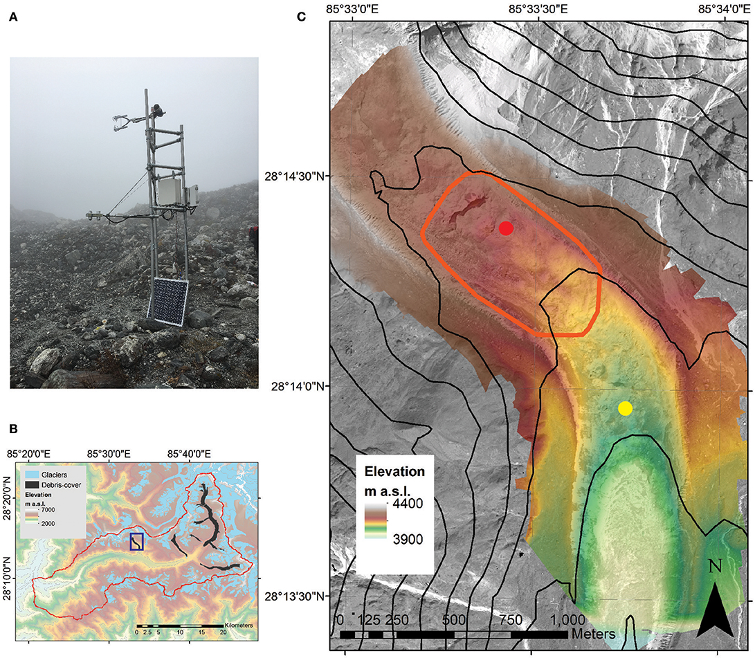
Figure 1. (A) AWS setup including CNR1 radiation sensor and eddy correlation sensor. (B) Map of the Langtang catchment, with Lirung glacier marked. (C) Map of Lirung glacier showing the location of the AWS (red spot) and the approximate outline of the thermal flights carried out during the measurement period (red polygon). The glacier tongue DEM is based on data collected by an unmanned aerial vehicle on the same day as the thermal flights, the background image of the surrounding area is a satellite image (SPOT) from October 2015. The yellow dot marks the location of the AWS from which data for the season of 2014 was available.
The local climate is dominated by monsoon circulation, with 68–89% of the annual precipitation falling between June and September (Immerzeel et al., 2014b), with a very rapid decrease in temperature, humidity and precipitation between the end of August until the end of October. The up valley winds typically transport moist air to higher altitudes resulting in condensation and generally overcast conditions in the afternoon. Due to the debris cover, surface temperatures increase well beyond air temperatures during the day (Steiner and Pellicciotti, 2016).
The location of the AWS was chosen on a location of the glacier that had several hundreds of meters relatively unobstructed fetch from the main wind direction.
The eddy correlation system was mounted onto the AWS tower. The tower is based on a modular design using three vertical anchors drilled into the ice and horizontal cross-pieces for stability (Jarosch et al., 2011). To install the tower, the debris was excavated and the vertical anchors were installed to a depth of 2 m using a manual ice auger. To limit melting of the tower into the ice, the ends were capped in plastic. After installation, the debris was replaced at the base of the tower.
At the AWS we measured incoming and outgoing shortwave and longwave radiation (1.6 m), relative humidity, air temperature measured at 10 min intervals (3.12 m) and wind speed components using an IRGASON sonic anemometer at 10 Hz (3.42 m, see Table 1 for sensor details). Temperatures within the debris were measured at depths of 0.15, 0.35, 0.55, and 0.75 m with TinyTag sensors. The debris thickness below the AWS is 0.75 m. We use the EddyPro Software (LI-COR, 2016) to calculate turbulent fluxes from the eddy correlation data. Fluxes were derived at 5 min intervals based on 10 Hz measurements of fluctuations in wind speed, humidity and temperature, then aggregated to 30 min values. Complete treatment included processes to remove trends and outliers. Linear detrending (Gash and Culf, 1996) was performed on the time series and spikes were removed based on Vickers and Mahrt (1997). We used planar-fit method, based on Wilczak et al. (2001), to rotate the coordinate system and derive the wind speed components and fluctuations. Wind measurements likely influenced by the mast structure or sensor tilt were removed by excluding all data points that were sourced within a 30° angle behind the sensor (Wilczak et al., 2001). High- and low-pass filters were applied based on Massman (2000) and Moncrieff et al. (2005) and density fluctuations were compensated based on Webb et al. (1980) accounting for attenuations of the fluxes due to sensor response, path length averaging and flux averaging periods.
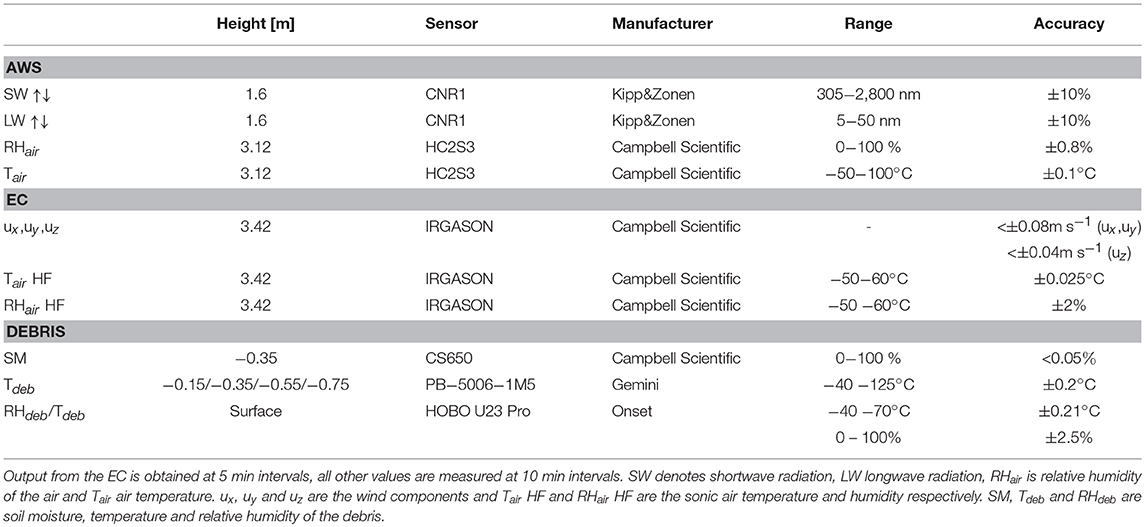
Table 1. Sensor specifications for relevant measurements at the AWS and eddy correlation system (EC) and in the debris.
In the subsequent year during the same season relative humidity and temperature measurements were carried out on the surface at the same location as the AWS, using a HOBO U23-Pro sensor.
Data from an AWS operational previously on the same glacier (Figure 1, 28.23260N, 85.56213E) from 4 May until 24 October 2014 was available to calculate bulk fluxes over a complete melting season. Sensor details are described in detail in Steiner et al. (2015).
Turbulent fluxes were estimated with the bulk aerodynamic method (Munro, 1989), using wind from the eddy correlation system and air temperature and humidity data from the AWS. Sensible and latent heat flux were calculated by
where H and LE are sensible and latent heat flux [W m−2], ρa is air density at the measurement site [kg m−3] calculated as where ρ0 is density [kg m−3] at standard sea level pressure p0 [1013.25 kPa] and p is pressure [Pa] measured at the site (Cuffey et al., 2010), u is wind speed [m s−1], Tz, Ts and qz, qs are the temperature [K] and specific humidity [-] at measurement height z [m] and the surface respectively. Ts is determined from the outgoing longwave radiation by inverting the Stephan Boltzman law, assuming an emissivity of 1. This estimate of Ts covers a larger footprint than a focused IR sensor. Le is the latent heat of vaporization for Ts >273.15 K (2.476 × 10⁶ kg J−1) and sublimation for Ts <273.15 K (2.830 × 10⁶ kg J−1) otherwise.
Cp is the specific heat capacity [J kg−1 K−1] of humid air calculated as
where cad is the specific humidity of dry air (1006 J kg−1 K−1).
Cbt denotes the bulk transfer coefficient. We test the three most commonly applied parametrizations of this bulk transfer coefficient (Fitzpatrick et al., 2017), namely one that does not include a stability correction, one that includes a stability correction based on the Richardson number and one that solves the MO length iteratively.
Some studies assume neutral stability over the debris cover (Nakawo and Young, 1982; Nicholson and Benn, 2006), which results in the straightforward calculations of Cbt excluding a stability function
where k is the von Kármán constant (0.41), zu and zt are the measurement heights [m] for wind speed as well as temperature and relative humidity respectively. z0m [m] is the surface roughness length of momentum, and z0t and z0q are the surface roughness lengths [m] for temperature and water vapor respectively, further discussed in section 4.2. Considering the large variations of surface temperature induced by the strong heterogeneous heating of the surface during the day (Brock et al., 2010; Steiner and Pellicciotti, 2016), a neutral boundary layer is unlikely and similarity theory imposes corrections for an unstable surface boundary layer. Two common methods exist to account for these stability effects. The first, employed over a debris-covered glacier before (Reid and Brock, 2010), is based on the Richardson number (Rib), where Cbt becomes
The stability functions are given by Brutsaert (1982) and used in similar context before (Favier et al., 2004; Brock et al., 2010)
where ϕm/h/v are the stability functions for momentum, heat and water vapor respectively and the Richardson number Rib (Moore, 1983; Brock et al., 2010) defined as
g is acceleration due to gravity [m s−2] and Tm [K] is the mean temperature between the measurement height z and the surface. Only values close to neutral atmospheric conditions (|Rib|<0.2) are considered.
The last approach is based on the MO stability parameter (z/L) resulting in
where and are the vertically integrated stability functions for momentum and heat (Brutsaert, 1982), with the stability function for water vapor to be assumed equal to the one for heat. L is the Obukhov length
where u* [m s−1] is the friction velocity. As L is a function of H itself an iterative process is needed to solve equations 1, 8, and 9. The stability functions are defined following Brutsaert (1992), developed specifically for the unstable layer, a situation to be expected for a warming debris-covered surface during the day.
Accurate modeling of turbulent fluxes depends on representative values for the roughness lengths of momentum (z0m), temperature (z0t) and water vapor (z0q) (Smeets et al., 1999; Smith, 2014). In former studies, for debris-covered glaciers either a constant value is used for z0m (Brock et al., 2006, 2010) or it has been estimated from high resolution DEMs for a specific field site (Rounce et al., 2015; Miles et al., 2017), then z0t and z0q were either assumed equal to z0m or an order of magnitude smaller. Due to the highly variable grain size of the debris cover, surface roughness varies considerably in space Miles et al. (2017), and since the spatial footprint of eddy correlation measurements changes in time this variability should be taken into account. We used a simple 2-dimensional model to estimate the footprint for each time step of atmospheric measurements (Kljun et al., 2015). The footprint is a transfer function f between 0 and 1 so that
where z0m is the effective surface roughness at the tower location, zl the local topographic roughness derived for the respective pixel and Ω denotes the integration domain, in this case the complete footprint. We estimated the boundary layer height to be at a maximum of 300 m, which corresponds to estimates based on Nieuwstadt (1981). Using a high-resolution DEM available for the field site (Immerzeel et al., 2014a) we derived distributed topographic roughness at a 2 m resolution, using the approach most closely matching measurements of z0m derived from wind tower measurements (Miles et al., 2017). We compared results from using this time series of z0m with those using a constant value of 0.03. We derived z0t and z0q applying a scaling relationship on z0m described in Smeets and van den Broeke (2008) for rough ice.
Turbulent latent heat flux calculations are a function of specific surface humidity (qs) which is difficult, if not impossible, to measure for the entire footprint of the flux measurements. No specific humidity measurements were available for the study period at the location of the AWS. Moreover, qs is highly variable due to variations in texture, from silt particles to large boulders, and the heterogeneous drying of the debris. Earlier studies have assumed the debris surface to be always fully saturated (Reid and Brock, 2010) or have considered two extremes ranging from fully saturated to a completely dry state (Nakawo and Young, 1982; Rounce et al., 2015). Collier et al. (2014) applied a numerical model to account for the diurnal drying of the debris, which is however relatively complex as our aim is to estimate the total energy for melt available on the debris surface. Recent literature examined links between surface temperatures and evaporation (Haghighi and Or, 2015a,b) and surface temperature measurements are relatively easy to carry out and even available at the spatially distributed scale (Kraaijenbrink et al., 2018). As the effective surface of the debris-cover surface is difficult to determine and hence representative measurements of humidity and corresponding temperature difficult to obtain we propose a semi-empirical solution based on Haghighi and Or (2015a). They provide a solution to quantify the water vapor gradient between the saturated surface and well mixed air above a viscous sublayer.
where Cs - Ca is the water vapor gradient through the sublayer [kg m−3], Mw is the molar mass of an evaporating liquid [kg mol−1], R is the universal gas constant [8.314 J mol−1 K−1] and RS is the air relative humidity at the top of the viscous sublayer, which corresponds to the effective relative humidity of the surface used to calculate the latent heat flux using the bulk approach. Psat(T) is the saturated vapor pressure estimated by the Antoine equation, a semi-empirical equation derived from the Clausius-Claperon relation.
where T is in [°C].
We solve equation 11 for RS and introduce parameters d for the unknown vapor gradient, e the vapor pressure term Psat(Ta) and f to scale the vapor pressure term Psat(Ts) leading to
Turbulent fluxes were measured for 13 consecutive days during the transition period between monsoon and post-monsoon (Figure 2). The period included days with clear skies and afternoon cloud formation due to anabatic valley circulation (27 and 30 September, 1 October, 10 and 11 October) as well as typical overcast monsoon days with high humidity, permanent cloud cover and low temperature variability (28 and 29 September, 2–9 of October; Figure 2). These overcast conditions are predominating in the monsoon dominated climate of the Nepalese Himalaya (Bonasoni et al., 2010; Forsythe et al., 2015; Shang et al., 2018). At the end of the period temperature and humidity decreased markedly while incoming radiative fluxes remained high. Sensible and latent heat are generally in the same order of magnitude and predominately negative, i.e., turbulent fluxes consistently removed energy from the debris surface.
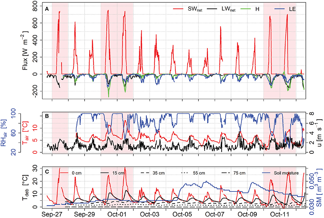
Figure 2. Fluxes and variables measured at the AWS, SWnet denoting net shortwave radiation, LWnet net longwave radiation, H sensible and LE latent heat flux (A). Climatic variables, including air temperature (Ta), wind speed (u), and relative humidity (RH) (B). Debris temperatures and soil moisture (SM) (C). The shaded time periods mark days we define as clear sky days, the others are overcast.
As incoming shortwave radiation increases, the debris surface quickly heats up to 30°C. Valley wind circulations lead to increased wind speeds and enhanced turbulent fluxes during the daytime. Relative humidity during the day quickly drops and rises again during clear days but remains saturated during overcast days often also during the day, resulting in a median full saturation. Winds on Lirung glacier are predominately anabatic, not in the direction of the glacier tongue but the valley itself, hence driven by larger convective patterns rather than local temperature gradients (Figure 3). The upslope valley winds persist and only weak katabatic winds form, likely because of the relatively warm debris surface even during the night.
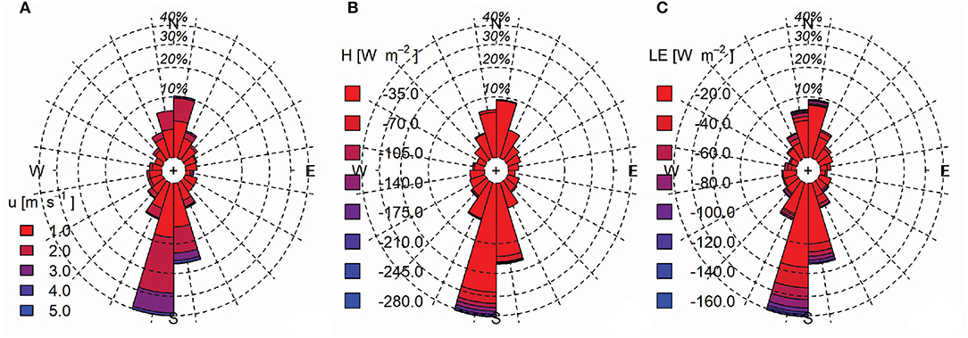
Figure 3. Wind velocities (A), sensible (B) and latent heat flux (C) relative to wind directions.
On clear sky days the sensible heat flux is more negative than latent heat due to the strong heating and quick drying of the surface, which is typical for debris (Steiner and Pellicciotti, 2016). During the day, when the glacier is sunlit, the sensible heat flux ranges between −179 ± 38 W m−2 around noon to −32 ± 18 W m−2 in the late afternoon (Figure 4). At night, between 5 pm and 6 am, sensible heat fluxes range from −10 ± 11 to 7 ± 15 W m−2. Latent heat fluxes reach values of about −102 ± 29 W m−2 at noon and decrease to −33 ± 9 and −3 ± 2 W m−2 at night (Figure 4). Because of the high relative values of the turbulent fluxes, the energy balance becomes negative around noon when incoming shortwave radiation starts to decline rapidly (Figure 5). Consequently, energy that can transit through the debris layer to melt the glacier ice is generated in the morning. Between 7 a.m. and 1 p.m., the net turbulent flux is on average lower than −150 W m−2 and the total net radiative balance is reduced between 17 and 125%.
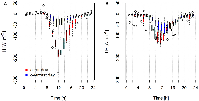
Figure 4. Measured sensible (A) and latent (B) heat fluxes on clear (red) and overcast (blue) days.
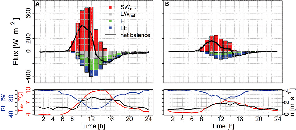
Figure 5. Median fluxes and meteorological data on (A) clear and (B) overcast days, with the net balance of all fluxes shown as a black line.
On an overcast day incoming shortwave radiation decreases from a median 846 ± 118 W m−2 to 221 ± 123 W m−2 (Figure 5). As a consequence the debris heats up less and sensible heat fluxes become smaller, reaching only −38 ± 18 W m−2 at noon up to positive values of 1.5±2 W m−2 at dawn. Latent heat plays a relatively larger role on overcast days, as daytime values reach beyond −50 W m−2 at noon (Figure 4). Between 7 a.m. and 1 p.m., the turbulent fluxes reduce the total net radiative flux by 20–74%. Under overcast conditions, due to the reduced turbulent fluxes, the positive net balance prolongs until 2 pm but reaches lower maximum values than during clear days (Figure 5).
The resulting observed evaporation rates, calculated by dividing the latent heat flux by water density and the latent heat of vaporization (2.476 MJ kg−1) over the debris surface are on average 2.8 and 1.8 mm w.e. day−1 on clear and overcast days, respectively. These values are higher than evaporation rates measured in the Tien Shan where Yao et al. (2014) report values between 0.9 and 1.9 mm w.e. day−1 and considerably higher than what has been observed on a debris-covered glacier in the European Alps, where Collier et al. (2014) report 0.6 to 0.9 mm w.e. day−1. Observations on a clean ice glacier show values of one order of magnitude lower (Kaser, 1982). Previously measured evaporation rates with a lysimeter on Lirung Glacier are one order of magnitude lower as well (Sakai et al., 2004), which could be explained by the lower wind speeds and temperature gradients that were observed. Extrapolated in space and time, evaporation may be an important mass flux on a debris-covered glacier in the Himalaya.
Sensible heat fluxes are comparable to the Tien Shan (Yao et al., 2014) but are lower than in the European Alps (Collier et al., 2014), most plausibly explained by the lower wind speeds as temperature gradients are likely higher in the Himalaya.
The total energy available for melt on the debris surface on clear (1.8 mm w.e. day−1) and overcast days (0.7 mm w.e. day−1) is considerably lower than if turbulent fluxes would be ignored (3 and 1.3 mm w.e. day−1 respectively).
The large negative flux between 1 pm and 7 pm could have implications for refreezing of liquid water present in the debris, a process so far rarely accounted for in debris energy balance models (Lejeune et al., 2013). Refreezing of water in the debris itself would have consequences for the conductivity, in turn influencing the energy transfer for melt to the debris-ice interface, while refreezing of melt water at the ice surface would reduce the total ablation directly.
Turbulent fluxes are closely correlated to the temperature difference between air and the surface both on clear (r = 0.94) and overcast (r = 0.85) days since it drives the sensible heat flux directly and the latent heat flux indirectly through the drying of the debris (Figure 6). While debris heats up quickly during the day due to direct solar radiation, after the sun has set it takes several hours before the positive surface to air difference disappears and the debris has cooled down. This retention of heat and a constant release through the afternoon explains why the overall net balance turns negative so early. Assuming full saturation of the surface, the relation to the specific humidity difference is strong for overcast days, where this assumption is valid most of the time but shows a large scatter on clear days, where the surface likely dries out considerably. The difference in atmospheric stability between these time periods explains the difference in correlation. This underlines the challenge of finding suitable stability corrections to accurately reproduce these fluxes during different and rapidly changing atmospheric conditions.
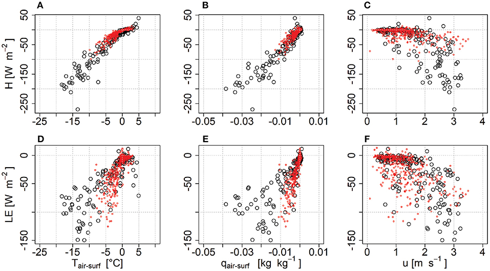
Figure 6. Half-hourly values for temperature difference between air and surface measurements (A,D) as well as specific humidity with the assumption of full saturation of the surface (B,E) and wind speed (C,F) compared to sensible (A–C) and latent heat flux (D–F). Red dots represent overcast while black dots represent clear sky days.
Debris temperatures in the upper 15 cm respond quickly to surface changes (Figure 2). This could be explained by latent heat fluxes contributing to a drier debris which eventually has a lower conductivity and hence a faster response to heating of the rocks but may also simply be due to the heating of the near-surface layers due to insolation. The relation between soil temperatures and soil humidity is not trivial (Whitaker, 1977) and goes beyond the scope of this study. Since drying and wetting originate from precipitation and drying from above, melting and freezing from the ice below as well as capillary action drawing moisture upwards from the debris-ice interface, it is difficult to quantify the moisture regime in the debris layer (Brutsaert, 2014; Collier et al., 2014). Continuous measurements of soil moisture at a depth of 35 cm show no clear relation to the fluxes on the surface (Figure 2), although days with especially low turbulent fluxes (29 September, 5, 6, and 9 October) coincide with wetting of the debris by precipitation, while the following days where the debris dries show increased fluxes. The weak relation between turbulent fluxes and soil moisture measurements is likely because this is beyond the horizon of influence of the surface fluxes or seen the other way around has little influence on the turbulent fluxes.
As the surface heats quickly, unstable conditions develop, resulting in mixing and higher wind speeds and increased turbulent fluxes (Figures 2, 3). This coincides also with stronger upvalley winds during the day that are likely a result of larger convective patterns, supplying more unsaturated air parcels.
The combination of slow cooling of the debris and sustained relatively high wind speeds into the afternoon (Figures 5, 6), maintain strong turbulent fluxes and cause the net balance to turn strongly negative from the early afternoon until the evening on most days. The relation between temperature and specific humidity differences and sensible heat are very strong, suggesting that measurements of these variables alone can give a good indication of the magnitude of the flux (Figure 6). As heating and drying of the debris becomes more heterogeneous on clear days and differences become generally much larger the scatter increases. This difference between clear and overcast days becomes even stronger for the latent heat flux, where the differences are good proxies on overcast days, but become much more variable as soon as the debris surface dries up (Figure 6). While stronger winds obviously do indicate greater turbulent fluxes, the relation is less distinct (Figure 6). Furthermore, situations with strong variation in temperature and specific humidity coincide with large instability and the assumption of stationarity may not hold anymore, causing correlation with the observations to deteriorate. This non-stationarity is facilitated by the heating as well as the large topographic variability of the debris surface. This in turn also explains why wind speeds measured at the point scale, do not accurately represent winds in the flux footprint, resulting in a poor correlation between wind and both turbulent fluxes.
Using the model proposed by Kljun et al. (2015) we calculate the footprint of the eddy correlation measurements at each time step. The model requires wind speed and direction, taken from measurements, u* [m s−1] and the Obukhov length L [m] and the standard deviation of lateral velocity fluctuations [m s−1] derived from the eddy correlation measurements and the boundary layer height assumed to be 300 m. The footprint provides a raster over the area around the AWS with each raster cell having a weight between 0 and 1 and all cells summing to unity (Equation 10). The representative roughness value of the whole footprint is then calculated by multiplying the weights with the respective topographic roughness from the gridded product. The resulting time series is relatively close to the initial constant value chosen and that provides confidence in the use of a constant value only (Figure 7). Previous energy balance studies of debris-covered glaciers assume the aerodynamic roughness length of temperature (z0t) and vapor (z0q) to be either equal to Schlögl et al. (2017) or one order of magnitude smaller than the roughness length of momentum (z0m). However, this factor is expected to be considerably lower for rough flow and high Reynolds numbers (Andreas, 2002; Smeets and van den Broeke, 2008). We use the Reynolds number calculated from flux measurements to derive the factor that is applied on the surface roughness length for momentum based on the relation found in Smeets and van den Broeke (2008) for rough ice and find a median value for the scalar of 0.05 ± 0.05, which we apply for all model runs.
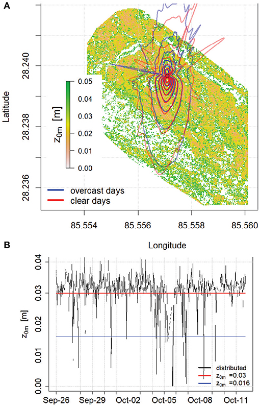
Figure 7. (A) Average footprint effective for the eddy correlation measurements visualized as contour lines for overcast and clear days during the study period. The contour lines delineate the 10–80% of the footprint area. Footprints outside the DEM domain are treated as NA. In the background the spatially distributed z0m is shown. (B) Time series of z0m obtained from the respective footprints (black) for each time step as well as the constant value used in this study (0.03, red) and in Brock et al. (2010); Reid and Brock (2010)) (0.016, blue).
Bulk model results with the assumption of a fully saturated surface are shown in Figures 8, 9 and statistics of the fit with measurements are provided in Table 2. The models work well in general but tend to overestimate peak values. All models tend to overestimate the maximum daily latent heat flux as the assumption of full saturation is not always valid, while on clear sky days the extreme temperature difference between debris surface and the air causes the bulk approach to overestimate the sensible heat flux. It is striking however that including the stability correction based on the Richardson number overestimates on average for all cases. Due to its restriction to near neutral conditions, ca 12% of the data points were already discarded a priori, if |Rib|>0.2. While the model results correlate well with measured fluxes for sensible heat (R2>0.8), the root mean square error (RMSE) is in the order of magnitude of the fluxes measured during the day. The models based on the Richardson number and without a stability correction also produce extreme spikes for latent heat fluxes, which have been reported previously (Brock et al., 2010) based on the same bulk approach and associated to strong evaporation after short rain events on the warm debris. However our comparisons between eddy correlation data and the bulk approach suggest that this is rather likely due to a structural overestimation of the model. We have as a consequence removed all values lower than −500 W m−2, which occurred 16 times for the latent heat flux in the these models, specifically on clear days, but only once for the model iterating over the MO length.
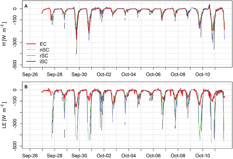
Figure 8. Model results for all bulk models over the whole study period for (A) sensible heat flux and (B) latent heat flux. EC denotes the eddy correlation measurements, nSC the model with no stability correction, rSC based on the Richardson number and iSC iterating over the Monin-Obukhov length. Timesteps with no data for a model are cases where it was below –500 W m−2.
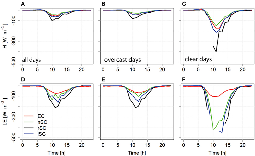
Figure 9. Diurnal cycles for all model results on all days (A,D), overcast days (B,E) and clear sky days (C,F) for sensible (A–C) and latent heat flux (D–F). EC denotes the eddy correlation measurements, nSC the model with no stability correction, rSC based on the Richardson number and iSC iterating over the Monin-Obukhov length. Timesteps with no data for a model are cases where all values were below –500 W m−2.
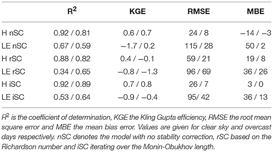
Table 2. Statistics of model performance for all days for both the latent and sensible heat flux for the three different models.
Additionally to the coefficient of determination (R2), the root mean square error (RMSE) and the mean bias error (MBE) we use the Kling-Gupta efficiency as an indicator for model performance, with 0 describing a situation where any random guess is as useful as the model and 1 a perfect prediction (Gupta et al., 2009). Both, the model without a stability correction and the model iterating over the MO length reproduce the sensible heat flux very well on all days, with an R2>0.8 and a RMSE<30 W m−2 for clear and <10 W m−2 for overcast days and a KGE>0.6 for all cases. They also perform well for the latent heat flux on overcast days, but overestimate the flux on clear sky days as the debris dries out, resulting in a RMSE between 95 and 115 W m−2 for the iterative approach and model without a stability correction respectively which is in the range of the highest measured values on these days. The MBE is 36 and 50 W m−2 respectively.
Comparing model performance to the temperature difference over the debris-covered tongue (Figure 10) shows that the model without a stability correction and the one based on the iteration over the MO length overestimate the sensible heat flux when the difference becomes large, however the one based on empirical parameters for the stability function (Equation 5) is especially off. This failure of models at large temperature gradients has been documented before for snow surfaces Schlögl et al. (2017). Comparing the results to the actual Richardson number reveals that as Rib becomes < 0, the offset increases. The empirical parameters in the function when derived for such large differences likely coincided also with higher wind speeds, typical for clear sky days with strong incoming solar radiation. The hummocky terrain of a debris-covered glacier prevents such high velocities to occur and hence makes the application of the approach using the Richardson number problematic. Similarly, the fact that the MO length measured at the eddy correlation system does not agree with the bulk model for which the Monin-Obukhov theory was developed (assuming constant flux layer and stationarity), introduced model uncertainties, which are difficult to quantify.
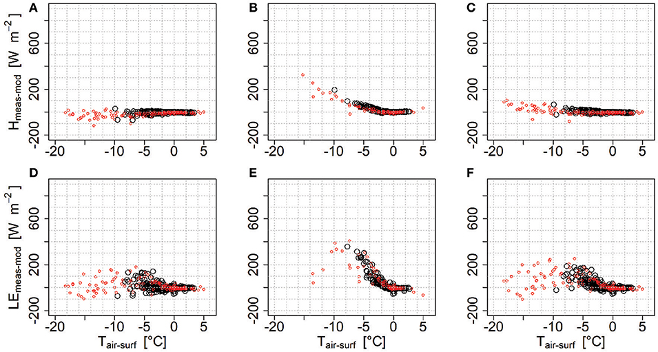
Figure 10. Differences in modeled and observed sensible (A–C) and latent (D–F) heat fluxes compared to the temperature difference measured between surface and air for the model with no stability correction (A,D), the model based on the Richardson number (B,E) and the model iterating over the Monin-Obukhov length (C,F). Colors denote clear sky (red) and overcast (black) conditions.
A similar relation between the temperature difference and the offset in the latent heat flux also is observed for all models. In this case, as the relation is especially strong on clear sky days, it can be explained with the indirect relation to the drying of the surface, as high surface temperatures caused by the incoming solar radiation cause the difference to rise and the debris to dry. In these cases the models, as they assume full surface saturation, overestimate the flux. Finding a relation between surface temperature and the observed specific humidity of the surface could therefore likely provide a possible improvement.
Given the difficulty in measuring accurate surface temperatures, the strongly heterogeneous surface roughness as well as the variable wind speed due to the hummocky terrain, we conduct a sensitivity analysis on these variables. We run the models with ±10% of the original value of temperature and wind speed. To account for the logarithmic effect we changed the log(z0m) ±50%, which corresponds to a range of z0m between 0.005 and 0.17, in line with observations of the observed spatial variability in the field Miles et al. (2017). We subsequently compare the effect on the mean of the overall fluxes. We only include the nSC and iSC models which performed reasonably well (Table 3).
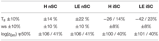
Table 3. Sensitivity of both turbulent fluxes to changes in input variables surface temperature (Ts), wind speed (ws) and surface roughness (z0m).
Results show that the models are very sensitive to surface temperature, as it is a strong direct driver of modeled fluxes (Figure 6). Note that a difference of 10% of surface temperature may occur regularly in practice due to shading and micro-relief (Steiner and Pellicciotti, 2016; Kraaijenbrink et al., 2018). Additionally, when using longwave radiation measurements to derive the surface temperature, uncertainties in emissivity cause a similar range of variation. To compare the surface temperature in the footprint of the eddy correlation measurements with the data measured at the station, we use distributed surface temperature measurements from three flights of an unmanned aerial vehicle with a thermal camera on 12 October at 7:30, 9 and 11 a.m. respectively (see Kraaijenbrink et al., 2018, for details on methods). Using the weighted footprint approach described in Kljun et al. (2015), we can derive the effective temperature at the site of the AWS, based on surface temperatures over the complete footprint and compare it to measurements taken at the station (Figure 11). The footprint at the first flight stretched only about 100 m south, while at the second and third flight covered the complete glacier toward the western moraine (ca 300 m) at a width of ca 150 m. While the overall range of temperatures in the footprints is large especially during the day, the point measurement at the AWS provides satisfying results. In the morning the temperature measured from the CNR4 underestimates the footprint temperature by 1.1°C (15%) at 7:30 a.m. and 2.4°C (19%) at 9 a.m. respectively, while by 11 a.m. the values correspond exactly. The underestimation in the morning is likely caused due to the station being shaded for a longer time. Turbulent fluxes at 7:30 are still negligible while at 09:30 the lower temperature used in bulk models could cause underestimations of fluxes beyond 20%, until the surface around the AWS heats up relatively to the rest of the glacier surface.
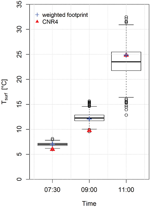
Figure 11. Surface temperatures measured by the UAV over the whole footprint at the corresponding time (boxplot), the corresponding weighted footprint temperature and the measurement from the AWS.
The fluxes are less sensitive to wind speed but the results are non-negligible as changes of ±10% can equally be caused by sensor inaccuracies. The hummocky terrain causes wind speeds to vary over the surface, as wind speeds are possibly larger on top of the debris mounds and lower in the depressions. Dadic et al. (2013) find that the sensitivity of turbulent fluxes increase with an increase in temperature and humidity, while for wind speed it peaks around 3–5 m s−1, which is largely beyond the wind speeds measured in our case. While further detailed analysis of the stability corrections is beyond the scope of this study, considering the large variety in debris surfaces when it comes to the local hummocky terrain and grain size, further sensitivities on idealized surfaces could provide insights for different climatic settings. Considering the variability of z0m observed on the footprint (Figure 6) as well as the variation among literature values (Nicholson and Benn, 2006; Brock et al., 2010; Reid and Brock, 2010; Rounce et al., 2015) the chosen range seems seems justified. Additionally the uncertainty of the factor to derive the roughness length of temperature and vapor is large as no further insight into their actual magnitude exists on debris cover, and studies over (rough) ice and snow suggest z0t to be possibly larger Calanca (2001), equal to Schlögl et al. (2017) or smaller than z0m Smeets et al. (1999). The results suggest that an accurate estimation of the roughness length is crucial for the derivation of turbulent fluxes using a bulk approach, as suggested earlier (Rounce et al., 2015).
The sensitivities reported in Table 3 have strong implications for distributed energy balance modeling, as all three variables vary in space. While z0m can be estimated with a topographic method (Miles et al., 2017), distributed wind measurements are less frequently available. A possible solution is the use of a large-eddy simulation (Sauter and Galos, 2016) to gain understanding in the wind distribution and its relation to the local topography. Distributed surface temperature measurements in time and space are difficult to obtain, although the use of thermal imagery from unmanned aerial vehicles is promising (Kraaijenbrink et al., 2018).
It is obvious from the results above that the models fail to reproduce latent heat fluxes during clear sky days when the surface dries out and the assumption of a saturated surface becomes invalid. Some of this offset can very likely be explained by inadequate stability corrections. One way to improve this would be to decrease z0q. However even decreasing it from z0q = 0.0015 to 10−5 only improves results marginally. We hence believe that the larger part of this discrepancy can be explained by our insufficient knowledge about surface drying. Since measuring surface specific humidity on a debris-covered glacier is difficult, we use surface temperatures as a proxy.
We derive the relative humidity of the surface required to model latent heat accurately with the bulk approach from the model without a stability correction by solving Equations 2 and 4 for the relative humidity, replacing the bulk flux of latent heat with the measured values. Placing these in equation 13, allows us to derive the parameters d = −0.13, e = 57 and f = 370. The data are shown in Figure 12. Measurements of surface humidity by a sensor placed within the rocks of the debris surface in the subsequent year during the same season and at the same location shows how measured values are higher for the same temperature, which is due to the gradient described in equation 11.
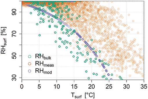
Figure 12. Relative humidity at the surface, necessary to fit the bulk model to eddy correlation measurements (RHbulk), measured embedded in the debris surface during a subsequent measurement campaign at the same location (RHmeas) and obtained using a regression based on (Haghighi and Or, 2015a) (RHmod).
Using a relative humidity value based on this equation, we are able to reduce the modeled latent heat fluxes considerably (Figure 13). As a result the RMSE for the model without a stability correction decreases from 115 to 45 W m−2 and the MBE decreases from 50 to 10 W m−2 on clear days. On overcast days the RMSE improved only marginally from 28 to 27 W m−2 and the MBE decreased from 2.1 to 1.4 W m−2. While still not accurately reproducing the fluxes on the hourly scale as the KGE only improved to 0.3 and R2 even dropped from 0.67 to 0.49 on clear days, it gives us more confidence of estimating the contribution of latent heat fluxes over a longer period of time.
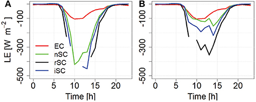
Figure 13. Diurnal cycles for the latent heat flux on clear days assuming full saturation (A) and relative humidity as a function of surface temperature (B). EC denotes the eddy correlation measurements, nSC the model with no stability correction, rSC based on the Richardson number and iSC iterating over the Monin-Obukhov length.
To assess the importance of turbulent fluxes over a complete melt season, we use the model without a stability correction to compute sensible and latent heat fluxes based on data from an AWS from May until October 2014 on the same glacier (Figure 1). We use the same parameters as before and model the surface relative humidity based on the model discussed above. We separate the data into the three distinct seasons, with pre-monsoon lasting from 4 until 14 June, monsoon from 15 June to 18 September and post-monsoon from the 19 September until 24 October. All fluxes including the measured net solar and net longwave radiation are shown in Figure 14.
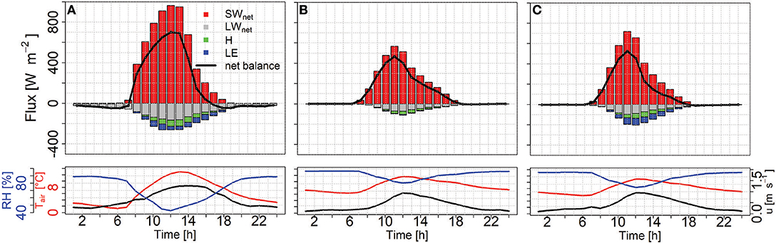
Figure 14. Energy balance on the glacier, with measured radiative fluxes and modeled turbulent fluxes based on AWS from 2014 during pre-monsoon (A), monsoon (B), and post-monsoon (C).
The location of the AWS in 2014, although only several hundred meters away, results in two distinct differences affecting the energy balance. First, net shortwave radiation is significantly higher, reaching 650 W m−2 in the post-monsoon season on average, while at the eddy correlation system such values were only reached on completely clear days. As the location is further up-glacier, it is shaded from the steep head walls most notably in the afternoon. Second, the AWS in 2014 was located in a depression resulting in wind speeds nearly half as low as at the location in 2016. As a result turbulent fluxes are considerably lower than at the measurement site from 2016. Nevertheless turbulent fluxes reduce the radiative fluxes between 7 a.m. and 5 p.m. by 5–66% in pre-monsoon, 0–12% in monsoon and 0–41% in post-monsoon. Over the entire melting season the turbulent fluxes reduce the total energy for melt available at the debris surface by 17%. During monsoon turbulent fluxes reach only 40 W m−2, largely because of a decreasing temperature gradient as the debris heats up less and an often saturated surface and very high air humidity, while wind speeds stay similar to the drier seasons. During both pre- and post-monsoon turbulent fluxes reach around 100 W m−2 between 10 a.m. and 4 p.m., with the latent heat flux being more important in the drying period in post-monsoon.
The aim of this study was to quantify turbulent fluxes over a debris-covered glacier by direct measurements with an eddy correlation system, test the accuracy of bulk models against these measurements and evaluate the contribution of turbulent fluxes to the energy balance at the debris surface. Direct measurements over a period of 16 days in the post-monsoon season in 2016 were investigated and compared against other climatic variables. Three separate bulk models, employing different parametrizations of the bulk transfer coefficient, were compared to eddy correlation measurements under different weather conditions. The best performing model was then used to evaluate turbulent fluxes over a complete melt season.
Our direct measurements of turbulent fluxes at the point scale show that turbulent fluxes are an essential part of the energy balance. Turbulent fluxes reduce the average net radiative flux input by 80% on clear days and 72% on overcast days, causing the total net surface balance to become negative very early in the afternoon, leaving only 5–7 h per day where the energy flux toward the debris is positive. While sensible heat fluxes are clearly the dominant turbulent flux on clear sky days, with values reaching up to −180 W m−2 during the day, the latent heat flux is dominant during overcast days and takes up more than 35% of the radiation input, resulting in evaporation rates between 1.8 mm day−1 on overcast and 2.8 mm day−1 on clear days.
We show that a frequently applied bulk approach using stability corrections based on the Richardson number performs poorly for large surface to air temperature differences, which are common on clear sky days. Since the original parametrization was likely developed for large differences in combination with high wind speeds, it fails for a debris-covered glacier where wind speeds remain relatively low even during the day. As a consequence the model overestimates turbulent fluxes by at least 100% during the day. The best performing models based on the same climate input data result in strong correlations for the sensible (>0.9 on clear sky and >0.8 on overcast days) and less strong for the latent heat flux (>0.5). The mismatch between model and observation is much larger for the latent heat flux because the specific humidity at the surface is below saturation during clear sky days, while the models assume full saturation. We however propose a simple parametrization based on the surface temperature that provides reasonable estimates for surface humidity and considerably improves the results on clear sky days. On overcast days the models overestimate the latent heat flux much less, with the best results provided by the model without a stability correction. This is encouraging, since most days during the melting season in High Mountain Asia are overcast, hence minimizing the error accrued over seasonal model runs. We conclude therefore that the bulk approach without a stability correction is the most suitable option for these hummocky surfaces with strong temperature differences and relatively low wind velocities.
We have used this model to calculate turbulent fluxes over a complete melt season at another location on the glacier. Because of its location in a depression at the lower tongue wind speeds were lower but incoming solar radiation higher. As a result absolute and relative turbulent fluxes were much lower at this location. However turbulent fluxes still reduced the radiative fluxes by up to 50% during the day and reduced the total energy for melt by 17% over the complete season.
It is therefore concluded that it is essential to include turbulent fluxes in melt calculations for debris-covered glaciers because they play a major role. Energy balance models for debris-covered surfaces as well as for cliffs and ponds that make use of the bulk approach should consider using the more suitable approach with no stability correction or a correction based on the MO length, rather than the Richardson parametrization, which could lead to significantly underestimated melt rates.
We also conclude that these models are very sensitive to both surface temperatures as well as wind speed and surface roughness, variables that strongly vary spatially over the glacier surface. Since the footprint for these turbulent fluxes covers a considerable surface even at these low wind speeds, an understanding of these variables in space is essential. While surface roughness can be estimated from the topography and we can show that point measurements of surface temperatures are good representations of temperatures in the footprint of the eddy correlation measurements, more efforts have to be invested to understand the surface boundary layer dynamics in order to produce reliable estimates of temperature and wind fields over such heterogeneous surfaces potentially using high resolution large-eddy simulations.
JFS wrote the initial version of the manuscript. ML, ES, JS, MB, and WI commented on the initial manuscript and helped improving this version. JFS developed the methodology with inputs from WI, MB, ML, and ES. JFS performed the analysis with support from WI, ML, and ES. All authors participated in fieldwork.
This project was supported by funding from the European Research Council (ERC) under the European Union's Horizon 2020 research and innovation program (grant agreement no. 676819) and by the research programme VIDI with project number 016.161.308 financed by the Netherlands Organisation for Scientific Research (NWO). This study was additionally supported by core funds of The International Centre of Integrated Mountain Development (ICIMOD) contributed by the governments of Afghanistan, Australia, Austria, Bangladesh, Bhutan, China, India, Myanmar, Nepal, Norway, Pakistan, Switzerland, and the United Kingdom.
The authors declare that the research was conducted in the absence of any commercial or financial relationships that could be construed as a potential conflict of interest.
We are grateful to the trekking agency Glacier Safari Treks and their staff without whom this work would not have been possible. We are grateful to GEMINI for providing the TinyTag sensors for this fieldwork. We are also grateful to our research partners, specifically Francesca Pellicciotti and Pascal Buri, for maintaining the AWS setup in 2014.
Andreas, E. L. (2002). Parameterizing scalar transfer over snow and ice: a review. J. Hydrometeorol. 3, 417–432. doi: 10.1175/1525-7541(2002)003<0417:PSTOSA>2.0.CO;2
Basnett, S., Kulkarni, A. V., and Bolch, T. (2013). The influence of debris cover and glacial lakes on the recession of glaciers in Sikkim Himalaya, India. J. Glaciol. 59, 1035–1046. doi: 10.3189/2013JoG12J184
Bolch, T., Kulkarni, A., Kääb, A., Huggel, C., Paul, F., Cogley, J. G., et al. (2012). The state and fate of Himalayan glaciers. Science 336, 310–314. doi: 10.1126/science.1215828
Bonasoni, P., Laj, P., Marinoni, A., Sprenger, M., Angelini, F., Arduini, J., et al. (2010). Atmospheric Brown Clouds in the Himalayas: First two years of continuous observations at the Nepal Climate Observatory-Pyramid (5079 m). Atmospheric Chemistry and Physics, 10, 7515–7531. doi: 10.5194/acp-10-7515-201
Brock, B. W., Mihalcea, C., Kirkbride, M. P., Diolaiuti, G., Cutler, M. E. J., and Smiraglia, C. (2010). Meteorology and surface energy fluxes in the 2005-2007 ablation seasons at the Miage debris-covered glacier, Mont Blanc Massif, Italian Alps. J. Geophys. Res. 115, D09106. doi: 10.1029/2009JD013224
Brock, B. W., Willis, I. C., and Sharp, M. J. (2006). Measurement and parameterization of aerodynamic roughness length variations at Haut Glacier d'Arolla, Switzerland. J. Glaciol. 52, 281–297. doi: 10.3189/172756506781828746
Brutsaert, W. (1982). Evaporation into the Atmosphere : Theory, History and Applications. Dordrecht: Springer Netherlands.
Brutsaert, W. (1992). Stability correction functions for the mean wind speed and temperature in the unstable surface layer. Geophys. Res. Lett. 19, 469–472. doi: 10.1029/92GL00084
Brutsaert, W. (2014). Daily evaporation from drying soil: universal parameterization with similarity. Water Resour. Res. 50, 3206–3215. doi: 10.1002/2013WR014872
Buri, P., Miles, E. S., Steiner, J. F., Brun, F., and Pellicciotti, F. (2016a). A physically-based 3D model of ice cliff evolution on a debris-covered glacier. J. Geophys. Res. Earth Surf. 121, 2471–2493. doi: 10.1002/2016JF004039
Buri, P., Pellicciotti, F., Steiner, J. F., Evan, S., and Immerzeel, W. W. (2016b). A grid-based model of backwasting of supraglacial ice cliffs on debris-covered glaciers. Ann. Glaciol. 57, 199–211. doi: 10.3189/2016AoG71A059
Calanca, P. (2001). A note on the roughness length for temperature over melting snow and ice. Q. J. R. Meteorol. Soc. 127, 255–260. doi: 10.1002/qj.49712757114
Collier, E., Nicholson, L. I., Brock, B. W., Maussion, F., Essery, R., and Bush, a. B. G. (2014). Representing moisture fluxes and phase changes in glacier debris cover using a reservoir approach. Cryosphere 8, 1429–1444. doi: 10.5194/tc-8-1429-2014
Conway, H., and Rasmussen, L. A. (2000). Summer temperature profiles within supraglacial debris on Khumbu Glacier, Nepal. Debris Covered Glaciers 89–97.
Conway, J. P., and Cullen, N. J. (2013). Constraining turbulent heat flux parameterization over a temperate maritime glacier in New Zealand. Ann. Glaciol. 54, 41–51. doi: 10.3189/2013AoG63A604
Cuffey, K. M. K., Paterson, W. S. B., Patterson, W. S. B., and Paterson, W. S. B. (2010). The Physics of Glaciers. 4 Edn., Burlington, NJ: Elsevier B.V.
Dadic, R., Mott, R., Lehning, M., Carenzo, M., Anderson, B., and Mackintosh, A. (2013). Sensitivity of turbulent fluxes to wind speed over snow surfaces in different climatic settings. Adv. Water Resour. 55, 178–189. doi: 10.1016/j.advwatres.2012.06.010
Denby, B., and Greuell, W. (2000). The use of bulk and profile methods for determining surface heat fluxes in the presence of glacier winds. J. Glaciol. 46, 445–452. doi: 10.3189/172756500781833124
Favier, V., Wagnon, P., Chazarin, J.-p., Maisincho, L., and Coudrain, A. (2004). One-year measurements of surface heat budget on the ablation zone of Antizana Glacier 15, Ecuadorian Andes. J. Geophys. Res. 109, 1–15. doi: 10.1029/2003JD004359
Fitzpatrick, N., Radić, V., and Menounos, B. (2017). Surface energy balance closure and turbulent flux parameterization on a mid-latitude mountain glacier, purcell mountains, Canada. Front. Earth Sci. 5:67. doi: 10.3389/feart.2017.00067
Forsythe, N., Hardy, A. J., Fowler, H. J., Blenkinsop, S., Kilsby, C. G., Archer, D. R., et al. (2015). A detailed cloud fraction climatology of the upper indus basin and its implications for near-surface air temperature. J. Clim. 28, 3537–3556. doi: 10.1175/JCLI-D-14-00505.1
Fyffe, C. L., Reid, T. D., Brock, B. W., Kirkbride, M. P., Diolaiuti, G., Smiraglia, C., and Diotri, F. (2014). A distributed energy-balance melt model of an alpine debris-covered glacier. J. Glaciol. 60, 587–602. doi: 10.3189/2014JoG13J148
Gardelle, J., Berthier, E., and Arnaud, Y. (2012). Slight mass gain of Karakoram glaciers in the early twenty-first century. Nat. Geosci. 5, 322–325. doi: 10.1038/ngeo1450
Gash, J. H. C., and Culf, A. D. (1996). Applying a linear detrend to eddy correlation data in realtime. Boundary Layer Meteorol. 79, 301–306. doi: 10.1007/BF00119443
Gupta, H. V., Kling, H., Yilmaz, K. K., and Martinez, G. F. (2009). Decomposition of the mean squared error and NSE performance criteria: Implications for improving hydrological modelling. J. Hydrol. 377, 80–91. doi: 10.1016/j.jhydrol.2009.08.003
Haghighi, E., and Or, D. (2015a). Thermal signatures of turbulent airflows interacting with evaporating thin porous surfaces. Int. J. Heat Mass Transfer 87, 429–446. doi: 10.1016/j.ijheatmasstransfer.2015.04.026
Haghighi, E., and Or, D. (2015b). Turbulence-induced thermal signatures over evaporating bare soil surfaces. Geophys. Res. Lett. 42, 5325–5336. doi: 10.1002/2015GL064354
Haidong, H., Yongjing, D., Shiyin, L., Han, H., Ding, Y., Liu, S., et al. (2006). A simple model to estimate ice ablation under a thick debris layer. J. Glaciol. 52, 528–536. doi: 10.3189/172756506781828395
Immerzeel, W. W., Kraaijenbrink, P., Shea, J. M., Shrestha, A. B., Pellicciotti, F., Bierkens, M. F. P., and de Jong, S. M. (2014a). High-resolution monitoring of Himalayan glacier dynamics using unmanned aerial vehicles. Remote Sens. Environ. 150, 93–103. doi: 10.1016/j.rse.2014.04.025
Immerzeel, W. W., Petersen, L., Ragettli, S., and Pellicciotti, F. (2014b). The importance of observed gradients of air temperature and precipitation for modeling runoff from a glacierized watershed in the Nepalese Himalayas. Water Resour. Res. 50, 2212–2226. doi: 10.1002/2013WR014506
Jarosch, A. H., Anslow, F. S., and Shea, J. M. (2011). “A versatile tower platform for glacier instrumentation: GPS and Eddy Covariance Measurements,” in Workshop on the Use of Automatic Measuring Systems Automatic Measuring Systems on Glaciers on Glaciers, IASC Workshop (Pontresina: IMAU), 52–55.
Kääb, A., Berthier, E., Nuth, C., Gardelle, J., and Arnaud, Y. (2012). Contrasting patterns of early twenty-first-century glacier mass change in the Himalayas. Nature 488, 495–498. doi: 10.1038/nature11324
Kaser, G. (1982). Measurement of Evaporation from Snow. Arch. Met. Geoph. BiokJ. Ser. B 30, 333–340. doi: 10.1007/BF02324674
Kljun, N., Calanca, P., Rotach, M. W., and Schmid, H. P. (2015). A simple two-dimensional parameterisation for Flux Footprint Prediction (FFP). Geosci. Model Dev. 8, 3695–3713. doi: 10.5194/gmd-8-3695-2015
Kraaijenbrink, P. D. A., Bierkens, M. F. P., Lutz, A. F., and Immerzeel, W. W. (2017). Impact of a global temperature rise of 1.5 degrees Celsius on Asia's glaciers. Nature 549, 257–260. doi: 10.1038/nature23878
Kraaijenbrink, P. D. A., Shea, J. M., Litt, M., Steiner, J. F., Treichler, D., Koch, I., and Immerzeel, W. W. (2018). Mapping surface temperatures on a debris-covered glacier with an unmanned aerial vehicle. Front. Earth Sci. 6:64. doi: 10.3389/feart.2018.00064
Lejeune, Y., Bertrand, J.-M., Wagnon, P., and Morin, S. (2013). A physically based model of the year-round surface energy and mass balance of debris-covered glaciers. J. Glaciol. 59, 327–344. doi: 10.3189/2013JoG12J149
LI-COR (2016). EddyPro. LI-COR, Inc; infrastructure for Measurements of the European Carbon Cycle consortium. Lincoln, NE: LI-COR, Inc.
Massman, W. J. (2000). A simple method for estimating frequency response corrections for eddy covariance systems. Agric. Forest Meteorol. 104, 185–198. doi: 10.1016/S0168-1923(00)00164-7
McCarthy, M., Pritchard, H., Willis, I., and King, E. (2017). Ground-penetrating radar measurements of debris thickness on Lirung Glacier, Nepal. J. Glaciol. 63, 543–555. doi: 10.1017/jog.2017.18
Mihalcea, C., Mayer, C., Diolaiuti, G., Lambrecht, A., Smiraglia, C., and Tartari, G. (2006). Ice ablation and meteorological conditions on the debris-covered area of Baltoro glacier, Karakoram, Pakistan. Ann. Glaciol. 43, 292–300. doi: 10.3189/172756406781812104
Miles, E. S., Pellicciotti, F., Willis, I. C., Steiner, J. F., Buri, P., and Arnold, N. S. (2016). Refined energy-balance modelling of a supraglacial pond, Langtang Khola, Nepal. Ann. Glaciol. 57, 29–40. doi: 10.3189/2016AoG71A421
Miles, E. S., Steiner, J. F., and Brun, F. (2017). Highly variable aerodynamic roughness length ( z 0 ) for a hummocky debris-covered glacier. J. Geophys. Res. Atmospheres 122, 1–20. doi: 10.1002/2017JD026510
Moncrieff, J., Clement, R., Finnigan, J., and Meyers, T. (2005). “Averaging, Detrending, and Filtering of Eddy Covariance Time Series,” in Handbook of Micrometeorology: A Guide for Surface Flux Measurement and Analysis, eds X. Lee, W. Massman and v. Law (Dordrecht: Springer Netherlands), 7–31.
Monin, A., and Obukhov, A. (1954). Osnovnie haraktristiki turbulentnogo peremeshivaniya v prizemnom sloe atmosferi [Main characteristics of turbulent mixing in atmospheric boundary layer]. Trudy Inst. Geofiz. (Akad. Nauk SSSR) 24, 163–187.
Moore, R. D. (1983). On the use of bulk aerodynamic formulae over melting snow. Nordic Hydrol. 14, 193–206. doi: 10.2166/nh.1983.0016
Munro, D. S. (1989). Surface roughness and bulk heat transfer on a glacier: comparison with eddy correlation. J. Glaciol. 35, 343–348. doi: 10.1017/S0022143000009266
Nakawo, M., and Young, G. (1982). Estimate of Glacier Ablation under the debris layer from surface temperature and meteorological variables. J. Glaciol. 28, 29–34. doi: 10.1017/S002214300001176X
Nicholson, L., and Benn, D. (2006). Calculating ice melt beneath a debris layer using meteorological data. J. Glaciol. 52, 463–470. doi: 10.3189/172756506781828584
Nieuwstadt, F. T. (1981). The steady-state height and resistance laws of the nocturnal boundary layer: theory compared with cabauw observations. Boundary Layer Meteorol. 20, 3–17. doi: 10.1007/BF00119920
Nuimura, T., Fujita, K., Fukui, K., Asahi, K., Aryal, R., and Ageta, Y. (2011). Temporal Changes in Elevation of the Debris-Covered Ablation Area of Khumbu Glacier in the Nepal Himalaya since 1978. Arctic Antarct. Alpine Res. 43, 246–255. doi: 10.1657/1938-4246-43.2.246
Østrem, G. (1959). Ice melting under a thin layer of moraine, and the existence of ice cores in moraine ridges. Geogr. Annaler 41, 228–230. doi: 10.1080/20014422.1959.11907953
Pellicciotti, F., Stephan, C., Miles, E., Herreid, S., Immerzeel, W. W., and Bolch, T. (2015). Mass-balance changes of the debris-covered glaciers in the Langtang Himal, Nepal, 1974-99. J. Glaciol. 61, 1–14. doi: 10.3189/2015JoG13J237
Radić, V., Menounos, B., Shea, J., Fitzpatrick, N., Tessema, M. A., and Déry, S. J. (2017). Evaluation of different methods to model near-surface turbulent fluxes for a mountain glacier in the Cariboo Mountains, BC, Canada. Cryosphere 11, 2897–2918. doi: 10.5194/tc-11-2897-2017
Ragettli, S., Bolch, T., and Pellicciotti, F. (2016). Heterogeneous glacier thinning patterns over the last 40 years in Langtang Himal. Cryosphere 10, 2075–2097. doi: 10.5194/tc-10-2075-2016
Reid, T. D., and Brock, B. W. (2010). An energy-balance model for debris-covered glaciers including heat conduction through the debris layer. J. Glaciol. 56, 903–916. doi: 10.3189/002214310794457218
Reid, T. D., and Brock, B. W. (2014). Assessing ice-cliff backwasting and its contribution to total ablation of debris-covered Miage glacier, Mont Blanc massif, Italy. J. Glaciol. 60, 3–13. doi: 10.3189/2014JoG13J045
Rounce, D. R., and McKinney, D. C. (2014). Debris thickness of glaciers in the Everest Area (Nepal Himalaya) derived from satellite imagery using a nonlinear energy balance model. Cryosphere 8, 1317–1329. doi: 10.5194/tc-8-1317-2014
Rounce, D. R., Quincey, D. J., and McKinney, D. C. (2015). Debris-covered glacier energy balance model for Imj–Lhotse Shar Glacier in the Everest region of Nepal. Cryosphere 9, 1–16. doi: 10.5194/tc-9-2295-2015
Sakai, A., Fujita, K., and Kubota, J. (2004). Evaporation and percolation effect on melting at debris-covered Lirung Glacier, Nepal Himalayas, 1996. Bull. Glacier Res. 21, 9–15.
Sakai, A., Nakawo, M., and Fujita, K. (1998). Melt rate of ice cliffs on the Lirung Glacier, Nepal Himalaya1996. Bull. Glacier Res. 16, 57–66.
Sakai, A., Takeuchi, N., Fujita, K., and Nakawo, M. (2000). “Role of supraglacial ponds in the ablation process of a debris-covered glacier in the Nepal Himalayas,” in Debris Covered Glaciers (Wallingford: IAHS), 119–130.
Sauter, T., and Galos, S. P. (2016). Effects of local advection on the spatial sensible heat flux variation on a mountain glacier. Cryosphere 10, 2887–2905. doi: 10.5194/tc-10-2887-2016
Schlögl, S., Lehning, M., Nishimura, K., Huwald, H., Cullen, N. J., Mott, R., and Ch, S. S. (2017). How do Stability Corrections Perform in the Stable Boundary Layer Over Snow? Boundary Layer Meteorol. 165, 161–180. doi: 10.1007/s10546-017-0262-1
Shang, H., Letu, H., Nakajima, T. Y., Wang, Z., Ma, R., Wang, T., et al. (2018). Diurnal cycle and seasonal variation of cloud cover over the Tibetan Plateau as determined from Himawari-8 new-generation geostationary satellite data. Sci. Rep. 8, 1105. doi: 10.1038/s41598-018-19431-w
Smeets, C. J., and van den Broeke, M. R. (2008). The parameterisation of scalar transfer over rough ice. Boundary Layer Meteorol. 128, 339–355. doi: 10.1007/s10546-008-9292-z
Smeets, C. J. P. P., Duynkerke, P. G., and Vugts, H. F. (1998). Turbulence characteristics of the stable boundary layer over a mid-latitude glacier. part i: a combination of katabatic and large-scale forcing c. j. p. p. smeets. Boundary Layer Meteorol. 87, 117–145. doi: 10.1023/A:1000860406093
Smeets, C. J. P. P., Duynkerke, P. G., and Vugts, H. F. (1999). Observed wind profiles and turbulent fluxes over an ice surface with changing surface roughness. Boundary Layer Meteorol. 92, 101–123. doi: 10.1023/A:1001899015849
Smith, M. W. (2014). Roughness in the earth sciences. Earth Sci. Rev. 136, 202–225. doi: 10.1016/j.earscirev.2014.05.016
Steiner, J., and Pellicciotti, F. (2016). On the variability of air temperature over a debris covered glacier , Nepalese Himalaya. Annals Glaciol. 57, 1–13. doi: 10.3189/2016AoG71A066
Steiner, J. F., Pellicciotti, F., Buri, P., Miles, E. S., Immerzeel, W. W., and Reid, T. D. (2015). Modelling ice-cliff backwasting on a debris-covered glacier in the Nepalese Himalaya. J. Glaciol. 61, 889–907. doi: 10.3189/2015JoG14J194
Vickers, D., and Mahrt, L. (1997). Quality control and flux sampling problems for tower and aircraft data. J. Atmospheric Oceanic Technol. 14, 512–526. doi: 10.1175/1520-0426(1997)014<0512:QCAFSP>2.0.CO;2
Webb, E., Pearman, G., and Leuning, R. (1980). Correction of flux measurements for density effects due to heat and water vapour transfer. Q. J. R. Meteorol. Soc. 106, 85–100. doi: 10.1002/qj.49710644707
Whitaker, S. (1977). Simultaneous heat, mass, and momentum transfer in porous media: a theory of drying. Adv. Heat Transf. 13, 119–203. doi: 10.1016/S0065-2717(08)70223-5
Wilczak, J. M., Oncley, S. P., and Stage, S. A. (2001). Sonic anemometer tilt correction algorithms. Boundary Layer Meteorol. 99, 127–150. doi: 10.1023/A:1018966204465
Keywords: debris-covered glaciers, turbulent fluxes, latent heat, sensible heat, surface energy balance, Himalaya
Citation: Steiner JF, Litt M, Stigter EE, Shea J, Bierkens MFP and Immerzeel WW (2018) The Importance of Turbulent Fluxes in the Surface Energy Balance of a Debris-Covered Glacier in the Himalayas. Front. Earth Sci. 6:144. doi: 10.3389/feart.2018.00144
Received: 26 March 2018; Accepted: 11 September 2018;
Published: 03 October 2018.
Edited by:
Michael Lehning, École Polytechnique Fédérale de Lausanne, SwitzerlandReviewed by:
Sebastian Schlögl, WSL Institute for Snow and Avalanche Research SLF, SwitzerlandCopyright © 2018 Steiner, Litt, Stigter, Shea, Bierkens and Immerzeel. This is an open-access article distributed under the terms of the Creative Commons Attribution License (CC BY). The use, distribution or reproduction in other forums is permitted, provided the original author(s) and the copyright owner(s) are credited and that the original publication in this journal is cited, in accordance with accepted academic practice. No use, distribution or reproduction is permitted which does not comply with these terms.
*Correspondence: Jakob F. Steiner, ai5mLnN0ZWluZXJAdXUubmw=
Disclaimer: All claims expressed in this article are solely those of the authors and do not necessarily represent those of their affiliated organizations, or those of the publisher, the editors and the reviewers. Any product that may be evaluated in this article or claim that may be made by its manufacturer is not guaranteed or endorsed by the publisher.
Research integrity at Frontiers
Learn more about the work of our research integrity team to safeguard the quality of each article we publish.