Forecasting Multiphase Magma Failure at the Laboratory Scale Using Acoustic Emission Data

Magmas fracture under high shear stresses, producing radiating elastic waves. At the volcano scale, eruption is often preceded by accelerating seismicity, while at the laboratory scales, sample failure appears to be preceded by similarly accelerating Acoustic Emission (AE). In both cases, empirical relationships between the acceleration and the time of the singular final event have offered tantalizing possibilities for forecast of eruptions and material failure. We explore the success of these tools in the laboratory by briefly reviewing datasets that have been presented previously and comparing the range of errors on forecast times with the range of errors associated with attempts to retrospectively forecast eruptions. We demonstrate that the heterogeneity of a system is crucial to making accurate forecasts on the sample scale, such that homogeneous systems are inherently unpredictable. We then analyse the effect of having an incomplete data sequence, as might be the case for real-time forecasting scenarios. We find that for heterogeneous systems, there is a critical proportion of the sequence that needs to have occurred before a forecast time converges on relatively low errors. As might be expected, the final portion of the sequence is the most important, while uncertainty on the start of the sequence is less important. Finally, we explore the simplest method for scaling the laboratory results to the volcano scenario.

Introduction

Volcanic eruptions affect ~600 million people worldwide (based on World Bank population data and the analyses of Small and Naumann, 2001; Auker et al., 2013), and yet the toolkit available for forecast of eruption times remains unreliable in many cases (see the analysis by Salvage and Neuberg, 2016). Most deterministic predictive tools are based on the observation that many geophysical signals (e.g., strain and seismicity) appear to accelerate toward a singular time, which coincides approximately with the onset of eruption (Voight, 1988; Voight and Cornelius, 1991; Kilburn and Voight, 1998; De la Cruz-Reyna and Reyes-Dávila, 2001; Kilburn, 2003; Ortiz et al., 2003; Smith et al., 2007; Smith and Kilburn, 2010; Bell and Kilburn, 2013; Boué et al., 2015; Salvage and Neuberg, 2016). This precursory phase of signal acceleration can last for minutes to years (Linde et al., 1993; Robertson and Kilburn, 2016). Accelerating signals can therefore be used to infer eruption timing ahead of the event itself, and in near real-time (Voight and Cornelius, 1991). In most cases, the feasibility of using these signals as predictors of eruption onsets has been assessed retrospectively, with variable success, such that real-time forecasting is not yet a useful reality.

A step forward can potentially be made if we understand the physical underpinning of the acceleration of volcanic signals toward eruption. The accelerating nature of certain geophysical signals toward a time-singularity has been interpreted to represent the coalescence of multiscale fracturing processes (Kilburn, 2003) scalable down to rock-fracturing processes in the laboratory (Voight, 1989; Smith et al., 2007; Benson et al., 2008; Lavallée et al., 2008). This implies that the empirical power-law relationships that generally describe failure phenomena in the lab or seismicity approaching an eruption could emerge from physically-grounded models for nucleation, growth and coalescence of small-to-large nested fracture systems, which has been shown to be the case for some rupturing systems (Main et al., 2017). This also means that there is a class of self-similarity across a truly vast range of scales, from samples just a few centimeters long in the laboratory, to volcanic conduits for which fracturing depths begin at 1,500 m and propagate to the surface during ascent (Neuberg et al., 2006; Thomas and Neuberg, 2012).

The scalability of laboratory signals to volcanic signals remains uncertain in detail, but hinges on the assumption that the point at which a rock or magma fails to remain load-bearing on a small scale, is analogous to the point at which fractures in magmatic systems become pervasive over much longer lengthscales, and an eruption can proceed by material failure (c.f. Kilburn, 2003; Neuberg et al., 2006). The scaling laws proposed are therefore relatively simple (Benson et al., 2008; Tuffen et al., 2008), and are repeated herein. However, it is clear that more laboratory work could bridge this scale gap more rigorously. For instance, laboratory investigation of fault rupture velocities in viscoelastic magma would permit to constrain slip rates in volcanic conduits in nature and would help refine those scaling laws as well as volcanic eruption forecasting models.

In this contribution, we summarize the technical insights that have arisen from the campaigns of laboratory investigation, which may shed light on volcanic precursory signal evolution. We contrast these with some of the geophysical observations made at the volcano-scale and show where the most compelling links have been made. We provide new analyses of the failure of heterogeneous rocks, and contrast those with relatively homogeneous systems across a range of volcanically-relevant textural complexity.

How Successful Have Retrospective or Real-Time Forecasting of Volcanic Eruptions Been?

A good starting point in assessing how successful mock-forecasts can be is when data have been acquired and can be analyzed retrospectively. We acknowledge that there may be a bias in the published work toward forecasts that are apparently successful, while less successful attempts are perhaps less likely to be reported. Marked exceptions to this are studies for which the central aim was to find methods of improvement of inaccurate forecasts such as Boué et al. (2015) and Salvage and Neuberg (2016).

If we take the time that an eruption has been forecast to have occurred as t_p and the actual eruption time observed as t_e, then we can take the error on the forecast as |t_e − t_p|/t_e. There are a few eruptions for which sufficient information exists that can be used to find this error magnitude on published retrospective forecast attempts, which are given in Table 1. We can see that the minimum error reported is as low as 0.002 for the Redoubt eruption in 1989–1990 (Voight and Cornelius, 1991) and as high as 0.36 for Pinatubo volcano erupting in 1991 (Bell et al., 2013). In these two cases the values refer to the minimum and maximum differences between the forecast and the eruption.

TABLE 1

Table 1. Accuracy of published retrospective eruption forecasts.

In general, there is little evidence in Table 1 that a particular volcano type, eruption style, or magma composition, results in a better predictability when using all the forecasts made. Rather, it seems more likely that variations on the error of any forecast is dominantly dependent on the placement and quality of instrumentation, the numerical forecasting technique applied (c.f. Bell et al., 2011 for a discussion of techniques), and perhaps the nature of the seismicity (all data, or discriminated datasets from picking of specific event types).

Quantitative Background

Here we aim to summarize the theoretical or empirical formulations that have been used to understand the phenomena of (1) magma or rock fracture, (2) empirical forecasting tools and probabilistic variations thereof, and (3) techniques to describe statistically heterogeneous materials. The latter is especially useful in linking the concepts in (1) and (2) as shown in part in Vasseur et al. (2017).

Rock and Magma Failure During Magma Ascent

Magmas ascend through the Earth's crust, during which both the country rock and the magma itself can break (Goto, 1999; Kilburn, 2003, 2012; Iverson et al., 2006; De Angelis and Henton, 2011; Thomas and Neuberg, 2012; Dmitrieva et al., 2013; Kendrick et al., 2014). In many cases, the seismic signals used to forecast eruptions are simply the entire aggregated number of events occurring in the vicinity of a volcano (as used in the original demonstration of Voight, 1988; Table 1). However, Neuberg et al. (2006) and Salvage and Neuberg (2016) demonstrate that low-frequency seismicity results from the repetitive fracturing events occurring at the same depth, interpreted to originate in the magma itself, and that these events are especially useful in retrospectively forecasting eruptions. Similarly, Kilburn (2003) points out that volcano-tectonic (VT) events resulting from rock fracture ahead of ascending magma must be the most useful seismic source for accelerating events that can be used to forecast the onset of a new eruption. Therefore, we expect that there is utility in low-frequency, magma-fracture events at established conduits exploited by fresh magma repetitively (e.g., at Soufriere Hills volcano, from 1995 onward), and in volcano-tectonic events leading to eruptions and originating from rock fracture ahead of new magma (e.g., Pinatubo, 1991). In either case, it is important to quantify the stress magnitudes necessary for fracturing to occur, which is also a useful comparison between the volcano- and laboratory-scale.

Magma is a viscoelastic fluid or suspension, which can fail in a brittle manner when shear stresses reach a critical value τ_s. For pure liquids without suspended bubbles or crystals, this value has been empirically found to be of order ${\tau }_s~10^8$ Pa, and varies between 100 and 300 MPa (Simmons et al., 1982; Webb and Dingwell, 1990; Cordonnier et al., 2012b; Wadsworth et al., 2018). Assuming that the liquid phase originates the fractures (acknowledging that crystals can break during flow of two-phase or multiphase magmas; Cordonnier et al., 2009; Deubelbeiss et al., 2011), we can parameterize these breaking stresses in terms of the physics of fracturing viscoelastic fluids. Assuming that Maxwell's viscoelastic model is appropriate, the breaking point has been found to occur at a single Deborah number, De = 10⁻² (c.f. Webb and Dingwell, 1990), where De is the ratio of the stress relaxation time λ_r and the stress accumulation time λ (Wadsworth et al., 2018). The stress relaxation time in Maxwell's model is λ_r = μ/G_∞, which contains the temperature- and composition-dependent liquid viscosity, μ, and the elastic shear modulus G_∞. The threshold De = 10⁻², implies that ${\tau }_s=10^{-2}{G}_{\infty }$, which is indeed ${\tau }_s~10^8$ Pa, when $G_{\infty }~10^{10}$ Pa across most silicate magmatic liquid compositions, and independent of temperature (Dingwell and Webb, 1990). Additional scaling for this threshold has been made for heterogeneous magmas involving crystals (Cordonnier et al., 2012a) and bubbles (Kameda et al., 2008). This threshold provides a clear magma strength that has been shown to be met at depth during magma ascent and is the proposed origin of some of the accelerating seismicity approaching eruption (Goto, 1999).

The onset of solid rock fracture also occurs at threshold stresses, which in the simplest view, depend on the lithostatic “confining” pressure, the pressure of fluids in the pore spaces and the driving distribution of shear stresses (Jaeger et al., 2009). Additionally, this depends on the size and volume fraction of heterogeneity elements in the material (Baud et al., 2014). In detail, it is the distance between two pre-existing cracks, two crystals or two bubbles—between elements of heterogeneity—that must be bridged in order for a system-spanning fracture to occur, and failure to ensue (Sammis and Ashby, 1986; Ashby and Sammis, 1990). As a leading example relevant to porous volcanic rocks, the unconfined compressive strength has the form ${\tau }_s=a{K}_{Ic}/({\varphi }^b\sqrt{\pi R})$, where a and b are empirical constants, R is the radius of the heterogeneity element, and K_Ic is the fracture toughness (in Pa.m^1/2), which scale with the volume fraction of heterogeneity ϕ (Sammis and Ashby, 1986; Zhu et al., 2011; Heap et al., 2016). Vasseur et al. (2017) found that these distances between textural heterogeneity elements control the strength predictably when used in conjunction with a scaled static fracture-mechanics model. In both the volcanic rock failure and magma failure, the value of strength is therefore highly dependent on ϕ, and, in detail, on the pore size distribution (Sammis and Ashby, 1986; Vasseur et al., 2017; Wadsworth et al., 2018). However, the magnitude of strength is similar at ${\tau }_s~10^2$ MPa when ϕ → 0.

The Forecasting Toolbox

Voight (1988) proposed an empirical relationship between the acceleration of an observable $\ddot{\Omega }$ and its rate $\stackrel{.}{\Omega }$, where we use dot-notation for time-derivatives. This has the general form

$\begin{array}{ll}\ddot{\Omega }=A{\stackrel{.}{\Omega }}^{\alpha }& \left(1\right)\end{array}$

where A and α are constants. Following Voight (1988), we can integrate (Equation 1) assuming that $\stackrel{.}{\Omega }={\stackrel{.}{\Omega }}_0$ at t = 0 to find solutions for α = 1 and α ≠ 1. Here ${\stackrel{.}{\Omega }}_0$ is the background event rate at t = 0. In most experimental scenarios, ${\stackrel{.}{\Omega }}_0=0$ at t = 0, but in the natural case, this may not be true (discussed later). Nevertheless, for α = 1, the result is an exponential increase of $\stackrel{.}{\Omega }$ with t of the form

$\begin{array}{ll}\stackrel{.}{\Omega }(t)=hexp(qt)& \left(2\right)\end{array}$

where h and q are constants. An exponential increase of $\stackrel{.}{\Omega }$ does not reach a singularity and so is only predictive of an eruption or of material failure if we define a critical $\stackrel{.}{\Omega }$ beyond which those critical events will occur. The more common case is that α > 1, which results in the commonly used Time-Reversed Omori Law (TROL; Kilburn, 2003; Bell et al., 2013, 2018)

$\begin{array}{ll}\stackrel{.}{\Omega }(t)=k{(t_c-t)}^{-p}& \left(3\right)\end{array}$

where k, t_c and p are constants that are allowed to freely vary such that best-fit values can be found. The constant p is equivalent to 1/(α − 1), used in previous work (Equation 1), and controls the non-linear shape of the approach of Ω to a singularity at t_c. This singularity represents a predictive quality of Equation (3) if we assume that a run-away to an infinite $\stackrel{.}{\Omega }$ must coincide with a run-away of behavior to eruption.

These two methods, the exponential (Equation 2) and the power-law (Equation 3), have a suite of fit-parameters that are not known a priori and therefore must be acquired by algorithmic fitting to data. Bell et al. (2013) demonstrated that statistically reliable fits can be found when a “Maximum Likelihood” (ML) method is applied to Equations (2) and (3). The ML parameters are those resulting in a model that gives the observed data the greatest probability and those that maximize the likelihood function. The parameters are adjusted by minimizing the negative log-likelihood function using a downhill simplex algorithm. The fundamental advantage of the ML method given here is that it does not require binning of Ω(t) data to get binned measures of $\stackrel{.}{\Omega }$, and can rather be used directly on the data themselves. Using this technique, for a time interval [t₀, t_n], the log-likelihood for Equation (2) can be written as (Bell, pers. comm.)

$\begin{array}{ll}ln(L)=q{\displaystyle \sum _{i=0}^n}{t}_i+nln(h)-\frac{h}{q}(exp(q{t}_n)-exp(q{t}_0))& \left(4\right)\end{array}$

where L is the likelihood and n is the number of events. The same approach can be taken with the power-law method (Equation 3), for which the log-likelihood becomes (Bell et al., 2013)

$\begin{array}{ll}ln(L)={\displaystyle \sum _{i=0}^n}ln(k{(t_c-t_i)}^{-p})+K& \left(5\right)\end{array}$

where

$\begin{array}{l}K=\{\begin{array}{l}k\left({(t_c-t_n)}^{1-p}-{(t_c-t_0)}^{1-p}\right)/\left(1-p\right)\text{ for }p\ne 1\\ k\left(\text{ln}(t_c-t_n)-\text{ln}(t_c-t_0)\right)\text{ for }p=1\end{array}\end{array}$

Finally, for consistency, it may be useful to define a linear evolution of $\stackrel{.}{\Omega }$ with t which is of $\stackrel{.}{\Omega }$ = c where c is a constant. As with the exponential model, it is not clear what use a linear model can be for forecasting critical events, but it nonetheless may be a reasonable descriptor of some datasets. For this,the log-likelihood is as follows (Bell, pers. comm.)

$\begin{array}{ll}\text{ln}(L)=nln(c)-c(t_n-t_0)& \left(6\right)\end{array}$

The best-fit ML parameters for each acceleration model are established by minimizing the negative of Equations (4–6). The observable Ω typically is an acoustic or seismic event count, such that it is a pure number. For this reason, here we do not present the non-cumulative best-fit models graphically because they are not informative—the clarity comes in cumulative form where the data are effectively stacked and elevated into a line with a given curvature. Moreover, as we have the advantage of working with non-binned data, there is no use in looking at a timeline of event timings, which is what non-cumulative data amount to. The cumulative form Λ of the exponential model (corresponding to Equations 2 and 4) is (Bell, pers. comm.)

$\begin{array}{ll}\Lambda (t)=\frac{h}{q}(exp(qt)-exp(q{t}_0))& \left(7\right)\end{array}$

That of the TROL (corresponding to Equations 3 and 5) is (Bell et al., 2013):

$\begin{array}{ll}\Lambda (t)=\frac{k}{p-1}({(t_c-t)}^{1-p}-{(t_c-t_0)}^{1-p})& \left(8\right)\end{array}$

And that of the constant rate model (corresponding to Equation 6) is:

$\begin{array}{ll}\Lambda (t)=c(t-t_0)& \left(9\right)\end{array}$

However, other metrics can be used such as strain, in the case of a constant driving-pressure scenario, or pressure, in the case of a constant displacement rate scenario. Other metrics that accelerate toward failure may exist. However, here we focus on event number as Ω. The energy of acoustic signals cannot be used in the same way because the ML method relies on the event timings in the log-likelihood function. In what follows we will test each of these approaches against a range of experimental datasets.

Describing Heterogeneous Magmas

Magmas may be heterogeneous in texture. While the most important distinguishing features might be identified on a volumetric basis, such as the gas volume fraction (or porosity) ϕ, or the crystal volume fraction ϕ_x, it may be important to understand the spatially defined properties. Examples are the frequency distribution of pore or crystal sizes, the distribution of inter-pore or inter-crystal distances, and degrees of anisotropy. Here we give the method described in Vasseur et al. (2017).

(Torquato et al., 1990) describe the void nearest-neighbor density function P(R) for a system of random heterogeneous overlapping particles with a characteristic radius R_p from which a pore-size density function can be derived (Torquato, 2013):

$\begin{array}{ll}\overline{P}\left(\overline{R}\right)=\frac{3\eta {\left(1+\overline{R}\right)}^2}{\varphi }exp\left(-\eta {\left(1+\overline{R}\right)}^3\right)& \left(10\right)\end{array}$

where $\overline{P}(\overline{R})=P(R)R_p$, $\overline{R}=R/R_p$ and η = −ln(ϕ). The first moment of Equation (10) allows us to compute the characteristic mean pore radius between the particles as follows

$\begin{array}{ll}\langle \overline{R}\rangle ={\displaystyle {\int }_0^{\infty }}\overline{R}\overline{P}(\overline{R})\text{d}\overline{R}.& \left(11\right)\end{array}$

Similarly, a single analytical expression for other metrics such as an inter-pore and an inter-particle distance can be derived from the first moment of a nearest neighbor function (Torquato et al., 1990):

$\begin{array}{ll}{\overline{l}}_i=\frac{\Gamma (4/3)}{{\eta }^{1/3}}& \left(12\right)\end{array}$

where Γ is the gamma function, and η = −ln(1 − ϕ) when i = 1 (the inter-pore distance; ${\overline{l}}_1=l_1/R$) and η = −ln(ϕ) when i = 2 (the inter-particle distance; ${\overline{l}}_2=l_2/R_p$). In porous volcanic rocks, Equations (10–12) result in typical inter-pore lengths $10^{-6}<l_1<10^{-4}$ m. We will use this range later in our discussion of data scaling from the laboratory to nature.

Experimental Methods

There is some commonality of technique among deformation testing equipment. First, most tests are performed on cylindrical samples in either uniaxial or triaxial deformation rigs (e.g., Vasseur et al., 2013; Heap et al., 2017). In AE studies of rock or magma fracture and failure, it is common to use piezoelectric transducers. In the case of high-temperature experiments, these can be in contact with the load frame or deformation pistons (Lavallée et al., 2008; Vasseur et al., 2015, 2017) or in direct contact with the sample or sample jacketing system via waveguides (Benson et al., 2008; Tuffen et al., 2008). Waveguides attenuate acoustic signals but do not alter frequency-amplitude ratios (Meredith and Atkinson, 1983).

The data presented herein (and from Vasseur et al., 2015, 2017) were collected using a uniaxial, high temperature, high load press built by Voggenreiter GmbH (Hess et al., 2007; see Figure 1 for a schematic). A linear variable differential transducer (LVDT) with a 150 mm travel range and a 10⁻⁶ m resolution is used to track displacement of the top piston. The force is monitored with a Lorenz Messtechnik GmbH K11 load cell with a range of 300 kN and an accuracy in either tension or compression of 0.05 % of the measured force. The rates of displacement are well-controlled in the range 8.3 × 10⁻⁷to 1 × 10⁻² m s⁻¹. A split 3-zone, 12 kW furnace (GERO GmbH) covers approximately 10 times the length of the sample and both pistons and can heat up to 1,100°C, accurate to within 2°C. With appropriate insulation, the stable hot zone is 0.12 m long. At the ends of both pistons, with a direct path through the pistons to the sample, are piezoelectric AE broadband transducers with 125 kHz central frequency. A 40 dB buffered preamplifier is used to transfer the AE signals to the Richter data acquisition system (Applied Seismology Consultants), recording an AE voltage continuously at 20 MHz sampling rate.

FIGURE 1

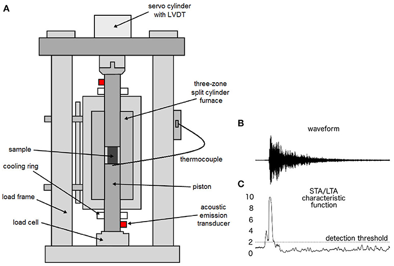
Figure 1. Experimental technique employed here. (A) The experimental set up at the Ludwig-Maximilians-Universität, Munich, showing a uniaxial press with high temperature furnace in the sample zone, capable of applying up to 300 kN. AE sensors are fitted at the top and bottom of the rig in direct contact with the single-piece pistons which in turn are in direct contact with the sample during operation. (B) An example waveform from a single experiment (see Figure 6). (C) The STA/LTA characteristic function showing that the detection threshold is exceeded at the onset of the AE event displayed in (B).

Some samples analyzed herein, and which appear in Vasseur et al. (2017), were deformed in a similar apparatus at the Laboratoire de Déformation des Roches (LDR) at the Université de Strasbourg. This device also used an LVDT transducer to measure displacement and piezoelectric transducers with central frequencies in the 100-1,000 kHz range to monitor AE signals. We refer the reader to Heap et al. (2015) for more details.

For all tests, cylindrical samples of ~ 10 mm radius and ~ 40 mm height were cored from blocks of (1) synthetic samples of welded glass beads (originally characterized in Vasseur et al., 2013; see Figure 2 for example 3D textures), or (2) volcanic rocks from Mt Meager volcano (Canada; Heap et al., 2014, 2015). We define the piston velocity as v = dL/dt and keep this constant during any test. The strain rate in the axial direction is then v/L₀, where L₀ is the starting sample length. The samples were deformed at (1) a strain rate of 10⁻³ s⁻¹ and a temperature of ~550°C (slightly above the glass transition onset in the viscoelastic regime) and (2) a strain rate of 10⁻⁵ s⁻¹ and under room temperature to ensure an elastic response. The temperature ~550°C is chosen to give an example condition typical of magma deformation, in which the sample is a relaxed liquid prior to deformation, but is driven to behave in a viscoelastic way by the application of a strain rate that is high compared with the relaxation time. At this temperature, the sample chosen has a viscosity of ~10¹² Pa s, and a relaxation time of 100 s, making the Deborah number De ≈ 0.1, which is above the critical value to ensure failure will ensue. AE event onsets were triggered and recorded automatically from the continuous acoustic datastreams using an adaptation of an autoregressive-Akaike-Information-Criterion (AR-AIC) picker (Beyreuther et al., 2010; Vasseur et al., 2015). The AR-AIC picker follows this workflow: (i) detection of the onset of a waveform above the baseline using an STA-LTA detector, (ii) de-noising of the acoustic signal, and (iii) AIC computation where the minimum indicates the arrival time. The STA-LTA window was set to 1 and 20 ms, respectively and the STA/LTA threshold was 2. The amplitude in dB and energy (typically in nJ), of each event were computed based on a resistance reference standard of 10 kΩ.

FIGURE 2

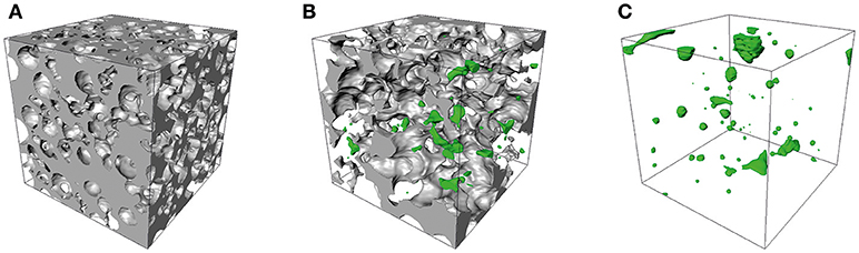
Figure 2. Example textures of variably porous sintered materials for which the pore space is rendered in 3-dimensions and colored gray if it is connected from edge-to-edge in any direction, or green if it is not. The porosities shown are (A) 0.460, (B) 0.290, and (C) 0.014. The box edge length is 0.3 mm. The non-pore phase (glass in this case) is made invisible for clarity. These textures are typical of the types of material microstructures that are deformed in the experiments presented herein and are especially relevant to granular or variably welded volcanic deposits. These images were obtained in situ at the Paul-Scherer-Institute (the Swiss Light Source beamline TOMCAT) and are taken with permission from Wadsworth et al. (2017).

All 42 samples were driven at constant rate as described above, until failure occurred where mechanical failure is defined as the point after which the sample is no longer load-bearing and the force drops to zero. This force-drop is easily picked in each mechanical dataset and provides excellent resolution on the measured t_c, which can then be compared with the predicted t_p using predictive tools described in section Quantitative Background.

Forecasting the Failure of Multiphase Magmas

We take a staggered approach to data analysis. First, we consider that effects of material heterogeneity on forecast efficacy can be best determined by using the complete data set of acoustic emissions (section The Effect of Porosity). However, we acknowledge that a true “forecast” would only be useful if it can be made before the final critical failure event has been reached, and therefore using less than the complete dataset. Therefore, in a second step, we analyse the effect of taking an incomplete sequence of data on the efficacy of forecasts (section Hindcasting or Simulated Forecasting).

The Effect of Porosity

Using datasets produced for deformation of sintered, variable porosity, variable grainsize, soda-lime silica glass beads (Vasseur et al., 2013, 2015), and natural sintered Mt Meager volcanic rock (Heap et al., 2015; Vasseur et al., 2017), we can apply the techniques described above to test the efficacy of failure forecast tools.

First, if we use 100% of the AE sequence, we can use the log-likelihoods given in Equations (4–6) to fit for the unknown constants in a linear form Equation (6), an exponential form Equation (4) and a power-law form Equation (5). In Figure 3 we plot the cumulative AE event number with time for low-to-high porosity samples for both sample types (sintered glass beads and welded volcanic debris from Mt Meager). The data are compared with the three model forms (Equations 7–9).

FIGURE 3

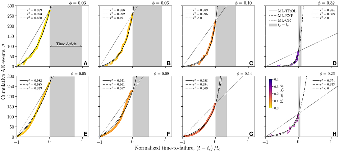
Figure 3. The cumulative number of AE events as a function of normalized time. For comparison the best-fit power-law (ML-TROL; Equation 8), exponential (ML-EXP; Equation 7), and linear models (ML-CR; Equation 9) are given. (A–D) are for synthetic samples of variably sintered soda-lime-silica glass beads (Vasseur et al., 2013, 2015). (E–H) are for variably welded natural samples of Mt Meager deposits (Heap et al., 2014, 2015). Each panel represents a different porosity sample with low porosity on the left and high porosity on the right. The gray shaded boxes represent the time difference between the observed failure time (left margin of the box) and the failure time predicted by the extrapolated singularity of the ML-TROL power-law model (right margin of the box), such that the box itself represents the time-deficit in the forecast. All panels contain information about the coefficient of determination r² obtained for each fit. Adapted from Vasseur et al. (2017).

The power-law (Equation 3) includes t_c as a fit-parameter, interpreted to be the best-fit modeled failure time (analogous to t_p described earlier). The value of t_p is much greater than the observed failure time t_c when the sample porosity is low (Figures 3A,E), creating a substantial time-deficit that equates to a poor predictability. However, as porosity is increased, t_p systematically approaches t_c (compare Figures 3A,E with Figures 3D,H) such that the time deficit is reduced and the potential for predictability is increased.

In the case of the linear and exponential forms, they fit the data better at low porosity than at high porosity. Therefore, it is clear that low-porosity samples do not deform with power-law precursory signals and rather the precursory signals follow exponential behavior. Indeed, at very low porosities, the data are almost linear (Figure 3E). This leads to the proposition that the power-law behavior in these critical mechanical systems is due to individually unpredictable events bridging gaps between textural flaws. And that the power-law predictability is an emergent property of a complex system, rather than intrinsic to material failure.

Hindcasting or Simulated Forecasting

In real forecasting scenarios at volcanoes, the beginning of the precursory sequence may not be detected, and similarly, by definition, a forecast requires that the end of the sequence is incomplete. Here we test these scenarios in which a data sequence may be partially incomplete and how such cases affect the efficacy of forecast times.

First, if we assume that we can rigorously define the beginning of the sequence, such that the initial time is well-defined, then we can test the effect of missing data at the end of the sequence. This is similar to real-time forecasting scenarios in which we might be acquiring new data in real time and adding it to the sequence and at each time-step, the fitting procedure would be repeated using (Equation 5). Examples of single low- and high-porosity data sets are given in Figures 4A,B (sintered glass beads) and Figures 4E,F (Mt Meager volcanic debris), in which fits to 100, 90, 80, and 70% of the time data are shown (given as fractions of the data sequence 0.7 ≤ f ≤ 1.0). The quality of the fits is similar from f = 1 down to f = f′ (where f′ is about 0.8 for the sintered glass beads and 0.9 for the welded volcanic debris), and the error on the forecast time is similar in that window. However, with sequences of less than f = f′, the forecast errors become larger for the high porosity samples. This indicates that the forecast efficacy is highly dependent on the amount of the sequence that has occurred, and that this dependence is stronger for high-porosity samples (see Figures 4C,G). Indeed, for f < f′, the dependence of forecast error on porosity is the inverse of the dependence found for f > f′, such that it would appear that high-porosity materials are less well-forecast than low-porosity materials. This also shows that the forecast error for high-porosity materials collapses to near zero as the sequence converges on t→t_c. Conversely, for low-porosity samples, we note that the inverse trend is observed, albeit with a lower degree: the variability in the forecast error grows as more and more of the sequence is acquired.

FIGURE 4

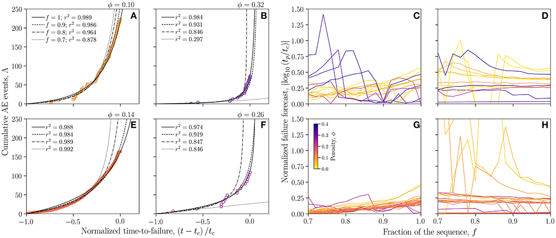
Figure 4. The effect of taking different fractions of a complete dataset. (A–D) are for the synthetic variably sintered glass bead samples, while (E–H) are for the variably welded Mt Meager datasets. Panels (A,B,E,F) are the data for two porosities, for which the ML-TROL power-law model is fit using increasing fractions of the data. f = 1 represents the full dataset, while f = 0.7, for example, would indicate that 70% of the total data set, measured from the beginning, has been used in the fitting. Panels (C,G) are the effect of taking increasing fractions of the data on the failure time accuracy. Contrastingly, in panels (D,H), the curves at f < 1 refers to a case when data at the beginning of the sequence is missing. A normalized failure forecast of unity (zero on this log axis), represents a perfect forecast. (A,B,E,F) contain information about the coefficient of determination r² obtained for each fit.

We also check the effect of missing the beginning of the sequence, analogous to missing low-amplitude events at the beginning of a precursory phase of activity at a volcano (especially problematic during long-duration precursory unrest phases; Robertson and Kilburn, 2016). In Figures 4D,H we show this effect is relatively independent of porosity and less important than the data accumulating at the end of the sequence.

Probability and Accuracy

For 0.7 ≤ f ≤ 1.0, we show in Figure 5 the effect of taking different proportions of the sequence on the forecast error. A complete sequence f = 1.0 relates to the forecast error for a complete sequence, and therefore represents a limiting case where the entire dataset is known ahead of time. Any reports of the predicted failure time for f = 1.0 are therefore not forecasts and are instead useful for assessing the quality of the functional forms for $\stackrel{.}{\Omega }(t)$ that could be used in forecasts. Here we see the strong dependence of the error on the sample porosity, with high-porosity materials being fully predictable with near-zero error. However, at f = 0.7, for which the uncertainty on the signal is higher, we note that the variability in the forecast error for high-porosity materials is larger than for materials with ϕ < 0.2, for which it becomes easier to forecast failure. We cast these as a Probability Density Function (PDF) of a given forecast error (Figure 5). For a given sample, we do this by sweeping over a range of initial guesses (using a reasonable initial value combined with a multiplicative factor varying between 1 and 10 every 0.05) on the fitted parameters in Equation (5), performing fits and computing the distribution of fitted forecast errors. The distribution is then converted to a PDF weighted by the coefficients of determination obtained from the fitting procedure. Displayed in Figure 5 is thus the intensity of the PDF obtained for each sample as a color map. The points represent the results obtained from using a single reasonable initial guess for each parameter and do not necessarily coincide with the most probable outcome.

FIGURE 5

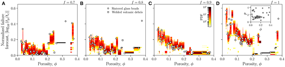
Figure 5. A probability map for what the likely error on a forecast time would be as a function of porosity. We give this for different fractions of a complete sequence in panels (A–D). A normalized failure forecast of unity (zero on this log axis), represents a perfect forecast. We show that there is a high probability of a perfect forecast at high porosities, but a low probability of good forecast at low porosities. See text for the details of the probability mapping. Inset to (D) shows the best-fit p exponent of the TROL obtained using (Equation 5) for f = 1.

Simple Scaling From the Lab to the Field

Across all values of porosity ϕ, the frequency F of the acoustic events in the laboratory-scale experiments detailed here ranged between F = 3 × 10⁴ and F = 1 × 10⁶ Hz. In Figure 6b we see that an additional complexity associated with high-porosity samples lies in the clear discrete onset being slightly masked compared with Figure 6a because the coda from the previous waveform overlaps with the onset of the new waveform.

FIGURE 6

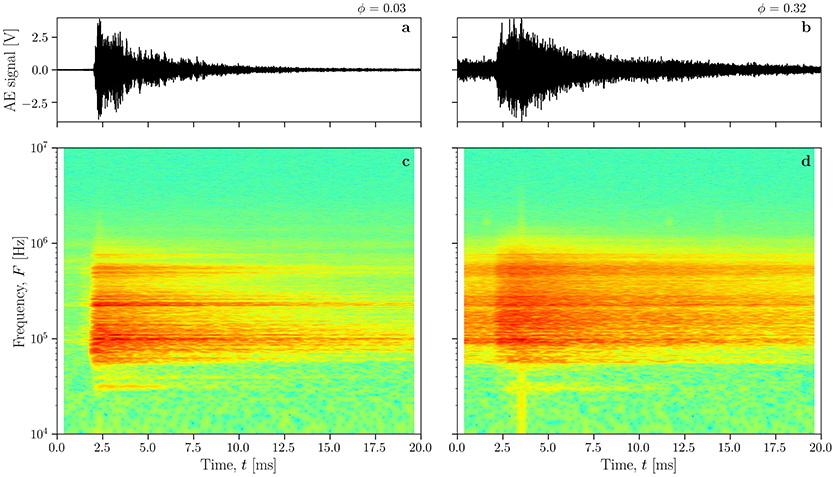
Figure 6. Typical waveforms for low porosity (a) and high porosity (b) samples with their related spectrograms (c,d), showing that the peak amplitude and frequency range does not significantly differ.

In other laboratory set-ups, events at much lower frequencies are detected; for example in Benson et al. (2008) and Tuffen et al. (2008), events as low as F = 10⁴ Hz, are found to be associated with pore fluid movement associated with sudden fracture propagation. This is only possible in pore-pressure controlled, jacketed triaxial experiments.

The scaling ratio most commonly deployed compares the product of a fracture lengthscale L and event frequency F at scale 1 to the same product at scale 2. This assumes that the fracture lengthscale is associated with the event that produced the signal frequency. If we use subscripts to denote the two scales, then this relation is L₁F₁ = L₂F₂ (Aki and Richards, 2002; Burlini et al., 2007). If scale 2 is the volcano scale, and scale 1 is the laboratory scale, then we can most easily place constraints on L₁, F₁, and F₂, and use these to predict L₂. If we stick to order-of-magnitude analysis, as shown above, $10^4\le F_1\le 10^6$ Hz and does not appear to depend on ϕ. We might expect that L₁ depends on ϕ and is the inter-pore length given by Equation (12). In a porous system, such as the sintered system used herein, we see that L₁ depends on the grainsize R. In natural sintered systems in volcanic environments, the grainsize is typically 10⁻⁵ < R < 10⁻³ m (Saubin et al., 2016). In turn, across the full range of ϕ from the initial packing ϕ down to low sintered ϕ > 0.03, using (Equation 12), we find that $10^{-6}\le L_1\le 10^{-4}$ m (see section Describing Heterogeneous Magmas). Finally, we know that VT events at volcanoes are typically 1 ≤ F₂ ≤ 10 Hz. This renders $10^{-3}<L_2<10^2$ m and gives insight into the fracture lengthscales between flaws on the volcano scale and is consistent with the pervasive fracture system lengthscales expected in some of the source-mechanism models for seismogenic eruptions (Neuberg et al., 2006). This also implies that while fracture lengths in the laboratory are typically related to the flaw or maximally, the sample lengths, at the volcano scale these would be much larger on the millimetric to hundred-meter scale. We work on the assumption that low-frequency magma-fracture events are damped events of an original VT-frequency content, congruent with the model of low-frequency events as magma rupture events (Neuberg et al., 2006; Thomas and Neuberg, 2012; Salvage and Neuberg, 2016).

A key difference between the laboratory cases presented here and natural cases is that laboratory experiments of this kind tend to be performed at a constant strain rate, allowing the stress to evolve in response, until failure. However, in nature, the magmatic conduit system may be more likely to be in a state of variable local strain rate (e.g., constant pressure at the conduit base or constant flux; c.f. Gonnermann and Manga, 2003). Future research should aim to explore scaling from laboratory to nature across a wide range of conditions and we identify this as a frontier topic.

Conclusions

We show that it is the heterogeneity of the system that most effects the efficacy of forecasts of material failure. Given this insight, we have presented the simplest scaling from the laboratory to the natural case on the basis of the relationship between rupture lengthscale and radiated frequency. On the laboratory scale, it is the inter-pore lengthscales that fail in each individual acoustic event, which leads to larger scale failure at the critical time. By scaling, we see that these events and the associated frequencies would be equivalent to seismic events at volcanoes with much larger rupture lengthscales. However, independent tests of the rupture lengthscales at active volcanoes are poorly known and would represent fruitful future work.

We explore the effect of having an incomplete dataset during a deformation episode. We find that the error on an attempted critical time forecast is substantially affected by missing data at the end of the sequence. The implication is that in any real-time scenario, the efficacy of the forecast will improve as the critical time approaches, especially for highly heterogeneous systems. Poor constraint on when the deformation episode began, however, is less important for effective forecasting.

We identify the specifics of scaling heterogeneities from the laboratory to nature as a frontier topic in need of attention. We propose that experimental work at larger scales could be used to validate the scale independence of forecast efficacies in highly heterogeneous systems, and explore the effect of system size on the forecasts possible in homogeneous systems. The ability to scale from laboratory findings to real crises in nature is critical.

Author Contributions

JV performed the experiments and processed the data. JV and FW conceptualized the study and analyzed the data. DD supervised the analysis. All authors contributed to the manuscript.

Conflict of Interest Statement

The authors declare that the research was conducted in the absence of any commercial or financial relationships that could be construed as a potential conflict of interest.

The reviewer, MF, declared a past co-authorship with one of the authors, DD, to the handling editor.

Acknowledgments

Thanks to three reviewers for thoughtful comments, and to Yan Lavallée, Ian G. Main, Andrew F. Bell, Caron Vossen, and Taylor Witcher for interesting discussions about forecasting rupture of geomaterials. We thank Mathieu Colombier for technical assistance with 3D data-rendering.

References

Aki, K., and Richards, P. (2002). Quantitative Seismology. Sausalito, CA.

Google Scholar

Ashby, M., and Sammis, C. (1990). The damage mechanics of brittle solids in compression. Pure Appl. Geophys. 133:489. doi: 10.1007/BF00878002

CrossRef Full Text | Google Scholar

Auker, M. R., Sparks, R. S. J., Siebert, L., Crosweller, H. S., and Ewert, J. (2013). A statistical analysis of the global historical volcanic fatalities record. J. Appl. Volcanol. 2:2. doi: 10.1186/2191-5040-2-2

CrossRef Full Text | Google Scholar

Baud, P., Wong, T., and Zhu, W. (2014). Effects of porosity and crack density on the compressive strength of rocks. Int. J. Rock Mech. Min. Sci. 67, 202–211. doi: 10.1016/j.ijrmms.2013.08.031

CrossRef Full Text | Google Scholar

Bell, A. F., and Kilburn, C. R. J. (2013). Trends in the aggregated rate of pre-eruptive volcano-tectonic seismicity at Kilauea volcano, Hawaii. Bull. Volcanol. 75:677. doi: 10.1007/s00445-012-0677-y

CrossRef Full Text | Google Scholar

Bell, A. F., Naylor, M., Heap, M. J., and Main, I. G. (2011). Forecasting volcanic eruptions and other material failure phenomena: an evaluation of the failure forecast method. Geophys. Res. Lett. 38:L15304. doi: 10.1029/2011GL048155

CrossRef Full Text | Google Scholar

Bell, A. F., Naylor, M., Hernandez, S., Main, I. G., Elizabeth Gaunt, H., Mothes, P., et al. (2018). Volcanic eruption forecasts from accelerating rates of drumbeat long-period earthquakes. Geophys. Res. Lett. 45, 1339–1348. doi: 10.1002/2017GL076429

CrossRef Full Text | Google Scholar

Bell, A. F., Naylor, M., and Main, I. G. (2013). The limits of predictability of volcanic eruptions from accelerating rates of earthquakes. Geophys. J. Int. 194, 1541–1553. doi: 10.1093/gji/ggt191

CrossRef Full Text | Google Scholar

Benson, P. M., Vinciguerra, S., Meredith, P. G., and Young, R. P. (2008). Laboratory simulation of volcano seismicity. Science 322, 249–252. doi: 10.1126/science.1161927

PubMed Abstract | CrossRef Full Text | Google Scholar

Beyreuther, M., Barsch, R., Krischer, L., Megies, T., Behr, Y., and Wassermann, J. (2010). ObsPy: a python toolbox for seismology. Seismol. Res. Lett. 81, 530–533. doi: 10.1785/gssrl.81.3.530

CrossRef Full Text | Google Scholar

Boué, A., Lesage, P., Cortés, G., Valette, B., and Reyes-Dávila, G. A. (2015). Real-time eruption forecasting using the material failure forecast method with a Bayesian approach. J. Geophys. Res. 120, 2143–2161. doi: 10.1002/2014JB011637

CrossRef Full Text | Google Scholar

Burlini, L., Vinciguerra, S., Di Toro, G., De Natale, G., Philip, M., and Burg, J.-P. (2007). Seismicity preceding volcanic eruptions: new experimental insights. Geology 35, 183–186. doi: 10.1130/G23195A.1

CrossRef Full Text | Google Scholar

Cordonnier, B., Caricchi, L., Pistone, M., Castro, J. M., Hess, K.-U., Gottschaller, S., et al. (2012a). The viscous-brittle transition of crystal-bearing silicic melt: direct observation of magma rupture and healing. Geology 40, 611–614. doi: 10.1130/G3914.1

CrossRef Full Text | Google Scholar

Cordonnier, B., Hess, K.-U., Lavallee, Y., and Dingwell, D. B. (2009). Rheological properties of dome lavas: case study of Unzen volcano. Earth Planet. Sci. Lett. 279, 263–272. doi: 10.1016/j.epsl.2009.01.014

CrossRef Full Text | Google Scholar

Cordonnier, B., Schmalholz, S. M., Hess, K.-U., and Dingwell, D. B. (2012b). Viscous heating in silicate melts: an experimental and numerical comparison. J. Geophys. Res. 117:B02203. doi: 10.1029/2010JB007982

CrossRef Full Text | Google Scholar

De Angelis, S., and Henton, S. M. (2011). On the feasibility of magma fracture within volcanic conduits: constraints from earthquake data and empirical modelling of magma viscosity. Geophys. Res. Lett. 38:L19310. doi: 10.1029/2011GL049297

CrossRef Full Text | Google Scholar

De la Cruz-Reyna, S., and Reyes-Dávila, G. A. (2001). A model to describe precursory material-failure phenomena: applications to short-term forecasting at Colima volcano, Mexico. Bull. Volcanol. 63, 297–308. doi: 10.1007/s004450100152

CrossRef Full Text | Google Scholar

Deubelbeiss, Y., Kaus, B. J. P., Connolly, J. A. D., and Caricchi, L. (2011). Potential causes for the non-Newtonian rheology of crystal-bearing magmas. Geochem. Geophys. Geosyst. 12, 1–22. doi: 10.1029/2010GC003485

CrossRef Full Text | Google Scholar

Dingwell, D. B., and Webb, S. L. (1990). Relaxation in silicate melts. Eur. J. Mineral. 427–449. doi: 10.1127/ejm/2/4/0427

CrossRef Full Text | Google Scholar

Dmitrieva, K., Hotovec-Ellis, A., Prejean, S., and Dunham, E. (2013). Frictional-faulting model for harmonic tremor before redoubt volcano eruptions. Nat. Geosci. 6, 652–656. doi: 10.1038/ngeo1879

CrossRef Full Text | Google Scholar

Gonnermann, H., and Manga, M. (2003). Explosive volcanism may not be an inevitable consequence of magma fragmentation. Nature volume 426, 432–435. doi: 10.1038/nature02138

CrossRef Full Text | Google Scholar

Goto, A. (1999). A new model for volcanic earthquake at Unzen Volcano: Melt Rupture Model. Geophys. Res. Lett. 26, 2541–2544. doi: 10.1029/1999GL900569

CrossRef Full Text | Google Scholar

Heap, M., Violay, M., Wadsworth, F., and Vasseur, J. (2017). From rock to magma and back again: the evolution of temperature and deformation mechanism in conduit margin zones. Earth Planet. Sci. Lett. 463, 92–100. doi: 10.1016/j.epsl.2017.01.021

CrossRef Full Text | Google Scholar

Heap, M. J., Farquharson, J. I., Wadsworth, F. B., Kolzenburg, S., and Russell, J. K. (2015). Timescales for permeability reduction and strength recovery in densifying magma. Earth Planet. Sci. Lett. 429, 223–233. doi: 10.1016/j.epsl.2015.07.053

CrossRef Full Text | Google Scholar

Heap, M. J., Kolzenburg, S., Russell, J. K., Campbell, M. E., Welles, J., Farquharson, J. I., et al. (2014). Conditions and timescales for welding block-and-ash flow deposits. J. Volcanol. Geotherm. Res. 289, 202–209. doi: 10.1016/j.jvolgeores.2014.11.010

CrossRef Full Text | Google Scholar

Heap, M. J., Wadsworth, F. B., Xu, T., Chen, C.-F., and Tang, C. (2016). The strength of heterogeneous volcanic rocks: a 2d approximation. J. Volcanol. Geotherm. Res. 319, 1–11. doi: 10.1016/j.jvolgeores.2016.03.013

CrossRef Full Text | Google Scholar

Hess, K.-U., Cordonnier, B., Lavallée, Y., and Dingwell, D. B. (2007). High-load, high-temperature deformation apparatus for synthetic and natural silicate melts. Rev. Sci. Instrum. 78, 75102–75104. doi: 10.1063/1.2751398

PubMed Abstract | CrossRef Full Text | Google Scholar

Iverson, R., Dzurisin, D., Gardner, C., Gerlach, T., LaHusen, R., Lisowski, M., et al. (2006). Dynamics of seismogenic volcanic extrusion at Mount St Helens in 2004–05. Nature 444, 439–443. doi: 10.1038/nature05322

PubMed Abstract | CrossRef Full Text | Google Scholar

Jaeger, J., Cook, N., and Zimmerman, R. (2009). Fundamentals of Rock Mechanics. Hoboken, NJ: Wiley.

Google Scholar

Kameda, M., Kuribara, H., and Ichihara, M. (2008). Dominant time scale for brittle fragmentation of vesicular magma by decompression. Geophys. Res. 35:L034530. doi: 10.1029/2008GL034530

CrossRef Full Text | Google Scholar

Kendrick, J. E., Lavallée, Y., Hirose, T., di Toro, G., Hornby, A. J., de Angelis, S., et al. (2014). Volcanic drumbeat seismicity caused by stick-slip motion and magmatic frictional melting. Nat. Geosci. 7, 438–442. doi: 10.1038/ngeo2146

CrossRef Full Text | Google Scholar

Kilburn, C. R. J. (2003). Multiscale fracturing as a key to forecasting volcanic eruptions. J. Volcanol. Geotherm. Res. 125, 271–289. doi: 10.1016/S0377-0273(03)00117-3

CrossRef Full Text | Google Scholar

Kilburn, C. R. J. (2012). Precursory deformation and fracture before brittle rock failure and potential application to volcanic unrest. J. Geophys. Res. 117:B02211. doi: 10.1029/2011JB008703

CrossRef Full Text | Google Scholar

Kilburn, C. R. J., and Voight, B. (1998). Slow rock fracture as eruption precursor at Soufriere Hills volcano, Montserrat. Geophys. Res. Lett. 25, 3665–3668. doi: 10.1029/98GL01609

CrossRef Full Text | Google Scholar

Lavallée, Y., Meredith, P. G., Dingwell, D. B., Hess, K.-U., Wassermann, J., Cordonnier, B., et al. (2008). Seismogenic lavas and explosive eruption forecasting. Nature 453, 507–510. doi: 10.1038/nature06980

PubMed Abstract | CrossRef Full Text | Google Scholar

Linde, A., Agustsson, K., Sacks, I., and Stefansson, R. (1993). Mechanism of the 1991 eruption of Hekla from continuous borehole strain monitoring. Nature 365, 737–740. doi: 10.1038/365737a0

CrossRef Full Text | Google Scholar

Main, I. G., Kun, F., and Bell, A. F. (2017). “Crackling noise in digital and real rocks–implications for forecasting catastrophic failure in porous granular media,” in Avalanches in Functional Materials and Geophysics, eds E. Salje, A. Saxena, and A. Planes (Cham: Springer), 77–97.

Google Scholar

Meredith, P. G., and Atkinson, B. K. (1983). Stress corrosion and acoustic emission during tensile crack propagation in Whin Sill dolerite and other basic rocks. Geophys. J. Int. 75, 1–21. doi: 10.1111/j.1365-246X.1983.tb01911.x

CrossRef Full Text | Google Scholar

Neuberg, J. W., Tuffen, H., Collier, L., Green, D., Powell, T., and Dingwell, D. B. (2006). The trigger mechanism of low-frequency earthquakes on Montserrat. J. Volcanol. Geotherm. Res. 153, 37–50. doi: 10.1016/j.jvolgeores.2005.08.008

CrossRef Full Text | Google Scholar

Ortiz, R., Moreno, H., García, A., Fuentealba, G., Astiz, M., Peña, P., et al. (2003). Villarrica volcano (Chile): characteristics of the volcanic tremor and forecasting of small explosions by means of a material failure method. J. Volcanol. Geotherm. Res. 128, 247–259. doi: 10.1016/S0377-0273(03)00258-0

CrossRef Full Text | Google Scholar

Robertson, R., and Kilburn, C. (2016). Deformation regime and long-term precursors to eruption at large calderas: Rabaul, Papua New Guinea. Earth Planet. Sci. Lett. 438, 86–94. doi: 10.1016/j.epsl.2016.01.003

CrossRef Full Text | Google Scholar

Salvage, R., and Neuberg, J. W. (2016). Using a cross correlation technique to refine the accuracy of the failure forecast method: application to Soufrière Hills volcano, Montserrat. J. Volcanol. Geotherm. Res. 324, 118–133. doi: 10.1016/j.jvolgeores.2016.05.011

CrossRef Full Text | Google Scholar

Sammis, C. G., and Ashby, M. F. (1986). The failure of brittle porous solids under compressive stress states. Acta Metall. 34, 511–526. doi: 10.1016/0001-6160(86)90087-8

CrossRef Full Text | Google Scholar

Saubin, E., Tuffen, H., Gurioli, L., Owen, J., Castro, J. M., Berlo, K., et al. (2016). Conduit dynamics in transitional rhyolitic activity recorded by tuffisite vein textures from the 2008–2009 Chaitén Eruption. Front. Earth Sci. 4:59. doi: 10.3389/feart.2016.00059

CrossRef Full Text | Google Scholar

Simmons, J. H., Mohr, R. K., and Montrose, C. J. (1982). Non-Newtonian viscous flow in glass. J. Appl. Phys. 53, 4075–4080. doi: 10.1063/1.331272

CrossRef Full Text | Google Scholar

Small, C., and Naumann, T. (2001). The global distribution of human population and recent volcanism. Glob. Environ. Chang. Part B Environ. Hazards 3, 93–109. doi: 10.1016/S1464-2867(02)00002-5

CrossRef Full Text | Google Scholar

Smith, R., and Kilburn, C. R. J. (2010). Forecasting eruptions after long repose intervals from accelerating rates of rock fracture: the June 1991 eruption of Mount Pinatubo, Philippines. J. Volcanol. Geotherm. Res. 191, 129–136. doi: 10.1016/j.jvolgeores.2010.01.006

CrossRef Full Text | Google Scholar

Smith, R., Kilburn, C. R. J., and Sammonds, P. R. (2007). Rock fracture as a precursor to lava dome eruptions at Mount St Helens from June 1980 to October 1986. Bull. Volcanol. 69, 681–693. doi: 10.1007/s00445-006-0102-5

CrossRef Full Text | Google Scholar

Thomas, M., and Neuberg, J. (2012). What makes a volcano tick—a first explanation of deep multiple seismic sources in ascending magma. Geology 40, 351–354. doi: 10.1130/G32868.1

CrossRef Full Text | Google Scholar

Torquato, S. (2013). Random Heterogeneous Materials: Microstructure and Macroscopic Properties. New York, NY: Springer Science and Business Media.

Google Scholar

Torquato, S., Lu, B., and Rubinstein, J. (1990). Nearest-neighbour distribution function for systems on interacting particles. J. Phys. A23:L103. doi: 10.1088/0305-4470/23/3/005

CrossRef Full Text | Google Scholar

Tuffen, H., Smith, R., and Sammonds, P. R. (2008). Evidence for seismogenic fracture of silicic magma. Nature 453, 511–514. doi: 10.1038/nature06989

PubMed Abstract | CrossRef Full Text | Google Scholar

Vasseur, J., Wadsworth, F. B., Heap, M. J., Main, I. G., Lavallée, Y., and Dingwell, D. B. (2017). Does an inter-flaw length control the accuracy of rupture forecasting in geological materials? Earth Planet. Sci. Lett. 475, 181–189. doi: 10.1016/j.epsl.2017.07.011

CrossRef Full Text | Google Scholar

Vasseur, J., Wadsworth, F. B., Lavallée, Y., Bell, A. F., Main, I. G., and Dingwell, D. B. (2015). Heterogeneity: the key to failure forecasting. Sci. Rep. 5:13259. doi: 10.1038/srep13259

PubMed Abstract | CrossRef Full Text | Google Scholar

Vasseur, J., Wadsworth, F. B., Lavallée, Y., Hess, K.-U., and Dingwell, D. B. (2013). Volcanic sintering: timescales of viscous densification and strength recovery. Geophys. Res. Lett. 40, 5658–5664. doi: 10.1002/2013GL058105

PubMed Abstract | CrossRef Full Text | Google Scholar

Voight, B. (1988). A method for prediction of volcanic eruptions. Nature 332, 125–130. doi: 10.1038/332125a0

CrossRef Full Text | Google Scholar

Voight, B. (1989). A relation to describe rate-dependent material failure. Science 243, 200–203. doi: 10.1126/science.243.4888.200

PubMed Abstract | CrossRef Full Text | Google Scholar

Voight, B., and Cornelius, R. R. (1991). Prospects for eruption prediction in near real-time. Nature 350, 695–698. doi: 10.1038/350695a0

CrossRef Full Text | Google Scholar

Wadsworth, F. B., Vasseur, J., Llewellin, E. W., Dobson, K. J., Colombier, M., Von Aulock, F. W., et al. (2017). Topological inversions in coalescing granular media control fluid-flow regimes. Phys. Rev. E96:033113. doi: 10.1103/PhysRevE.96.033113

CrossRef Full Text | Google Scholar

Wadsworth, F. B., Witcher, T., Vasseur, J., Dingwell, D. B., and Scheu, B. (2018). “When does magma break?” in Advances in Volcanology, eds J. Gottsmann, J. Neuberg, and B. Scheu (Berlin; Heidelberg: Springer).

Webb, S. L., and Dingwell, D. B. (1990). Non-Newtonian rheology of igneous melts at high stresses and strain rates: experimental results for rhyolite, andesite, basalt, and nephelinite. J. Geophys. Res. 95, 15695–15701. doi: 10.1029/JB095iB10p15695

CrossRef Full Text | Google Scholar

Zhu, W., Baud, P., Vinciguerra, S., and Wong, T.-F. (2011). Micromechanics of brittle faulting and cataclastic flow in Alban Hills tuff. J. Geophys. Res. 116:B06209. doi: 10.1029/2010JB008046

CrossRef Full Text | Google Scholar