 Adrien Napoly
 Tom Grassmann
 Fred Meier
 Daniel Fenner
- 1CNRM UMR 3589, Météo France/CNRS, Toulouse, France
- 2Chair of Climatology, Institute of Ecology, Technische Universität Berlin, Berlin, Germany
In urban areas, dense atmospheric observational networks with high-quality data are still a challenge due to high costs for installation and maintenance over time. Citizen weather stations (CWS) could be one answer to that issue. Since more and more owners of CWS share their measurement data publicly, crowdsourcing, i.e., the automated collection of large amounts of data from an undefined crowd of citizens, opens new pathways for atmospheric research. However, the most critical issue is found to be the quality of data from such networks. In this study, a statistically-based quality control (QC) is developed to identify suspicious air temperature (T) measurements from crowdsourced data sets. The newly developed QC exploits the combined knowledge of the dense network of CWS to statistically identify implausible measurements, independent of external reference data. The evaluation of the QC is performed using data from Netatmo CWS in Toulouse, France, and Berlin, Germany, over a 1-year period (July 2016 to June 2017), comparing the quality-controlled data with data from two networks of reference stations. The new QC efficiently identifies erroneous data due to solar exposition and siting issues, which are common error sources of CWS. Estimation of T is improved when averaging data from a group of stations within a restricted area rather than relying on data of individual CWS. However, a positive deviation in CWS data compared to reference data is identified, particularly for daily minimum T. To illustrate the transferability of the newly developed QC and the applicability of CWS data, a mapping of T is performed over the city of Paris, France, where spatial density of CWS is especially high.
Introduction
Dense atmospheric observational networks providing high-quality data are still a challenge today, especially in urban areas where spatial heterogeneity of surface cover and surface structures lead to a distinct spatial distribution of air temperature (T) (Oke, 1982). While for some cities high-density networks such as the Birmingham Urban Climate Laboratory (Chapman et al., 2015) are available, high costs to deploy and maintain them over time have limited their number (Chapman et al., 2015; Muller et al., 2015). As a result, many cities have only a few measurement sites, often only one single station (e.g., airport), or even none at all.
The term “crowdsourcing” has been[200mm][-12mm] Q22 defined by Howe (2006) as a web-based business model that uses a distributed network of individuals to obtain data. It was then specified by Muller et al. (2015) for atmospheric science as obtaining data through non-traditional and large number of sources, notably public sensors connected by the internet. The use of crowdsourced data is yet relatively new in atmospheric research (Bell et al., 2013; Overeem et al., 2013) compared to other scientific disciplines such as biology or astrophysics (Dickinson et al., 2010; Cook, 2011). However, the potential of such data has already been shown, notably for T observations (Chapman et al., 2017; Droste et al., 2017; Fenner et al., 2017; Meier et al., 2017), pressure observations (Madaus et al., 2014; Kim et al., 2016; McNicholas and Mass, 2018) or precipitation measurements (De Vos et al., 2017) in urban environments, and hence crowdsourcing could be an approach to overcome the limitations induced by traditional networks.
The benefit of crowdsourced data in atmospheric research lies in high spatial resolution and extended coverage in urban areas, potentially long-term measurements, and low cost that it provides compared to traditional networks. However, the most critical issue is found to be the quality of data from such networks (Bell et al., 2015; Chapman et al., 2017; De Vos et al., 2017; Meier et al., 2017). As crowdsourced data are directly collected by citizen weather stations (CWS) owned by individuals of the crowd, there is no or very little external control to ensure the quality of the obtained data set and hence data quality assessment is a crucial step before any analysis can be carried out (Chapman et al., 2017; Meier et al., 2017). Chapman et al. (2017), e.g., studied T in London, United Kingdom, using CWS data by removing measurements from their data set if the temporal average deviated more than three times the standard deviation of the average of all stations. Meier et al. (2017) accurately addressed the issue of quality assessment of crowdsourced CWS data, suggesting a detailed approach to identify suspicious crowdsourced T and filter these from the data set. Their method relies mostly on data from a quality-controlled reference network that allows them to exclude the suspicious CWS measurements. Main error sources were not due to the quality of the sensor itself but mostly related to the siting of the CWS (Meier et al., 2017), i.e., (i) the CWS are not always set up outside, and (ii) some stations are influenced by solar radiation leading to radiative errors. Recently, Hammerberg et al. (2018) applied a modified version of this QC approach to quality-control CWS data in Vienna, Austria, also including a statistically-based QC step that relies on the distribution of T data. While these QC procedures (Meier et al., 2017; Hammerberg et al., 2018) specifically address and identify common error sources in CWS data by using reference data, the methods can only be applied in other urban regions where high-quality reference data are available from multiple stations in different environments. This, of course, hinders the transferability due to the lack of detailed reference data in most cities. Therefore, in the current study, a new statistically-based QC approach is proposed for crowdsourced T data that is independent of such detailed reference networks.
Crowdsourced T data from Netatmo CWS (https://www.netatmo.com/) are used in this study, as these stations are distributed worldwide with a high spatial density especially in European cities, and the data can easily and freely be accessed via an API (Meier et al., 2017). The objectives of this study are to address the quality assessment of this data set by developing a new QC procedure based on a statistical analysis that (i) does not need a set of reference data, (ii) is robust and can be applied in different cities, and (iii) can easily be applied in future studies. The cities of Berlin, Germany, and Toulouse, France, are in this way investigated during a 1-year period (July 2016 to June 2017). First, the newly developed QC is evaluated and compared with the method developed by Meier et al. (2017). Second, a detailed comparison between T observed by CWS and reference networks is performed for an assessment of the quality-controlled crowdsourced data sets. Third, to illustrate the transferability and a possible application of CWS, a mapping of T is performed over the city of Paris, France, using quality-controlled CWS data.
Materials and Methods
Study Areas and Period
Two cities are investigated in this study for the development of the QC: Berlin, Germany (52.52° N, 13.40° E) and Toulouse, France (43.60° N, 1.45° E). They were chosen for two reasons: (i) their climatic and topographic similarities, i.e., weak influence of mountains or seas, overall relatively flat topography, and a humid warm temperate climate (Cfb) according to Köppen's classification (Kottek et al., 2006), (ii) the availability of CWS data with a high number of stations, and (iii) the availability of reference networks (more details in section Reference data sets). However, the two cities also exhibit morphologic differences, i.e., size, population and thus density of their CWS networks. The main characteristics of the two cities are summarized in Table 1. The investigated period lasts one year, from 1 July 2016 to 30 June 2017.
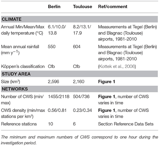
Table 1. Main characteristics of the two investigated cities.
Reference Data Sets
Quality-controlled reference measurements were used to evaluate the performance of the new QC. In Berlin, the reference data set consists of six stations maintained by the Chair of Climatology at Technische Universität Berlin (Urban Climate Observation Network–UCON; Fenner et al., 2014), and four stations maintained by the German weather service (DWD) (Figure 1, right and Table A1 in Supplementary Material). Note that only stations set up in built-up local climate zone (LCZ) classes were considered, using the LCZ classification in Fenner et al. (2017). UCON measurements are taken by Campbell Scientific CS215 T and relative humidity probes (specified accuracy ± 0.4 K in range 5–40°C) at 1-min resolution, fixed in white radiation shields that are actively ventilated during sunlit periods. These data were calibrated and quality controlled as described in Meier et al. (2017), and aggregated to hourly mean values. DWD measurements are taken with Eigenbrodt LTS2000 T probes (specified accuracy ± 0.2 K), fixed in actively-ventilated white radiation shields. Data are provided as quality-checked products (Kaspar et al., 2013; DWD Climate Data Center, 2017) at one-hourly resolution.
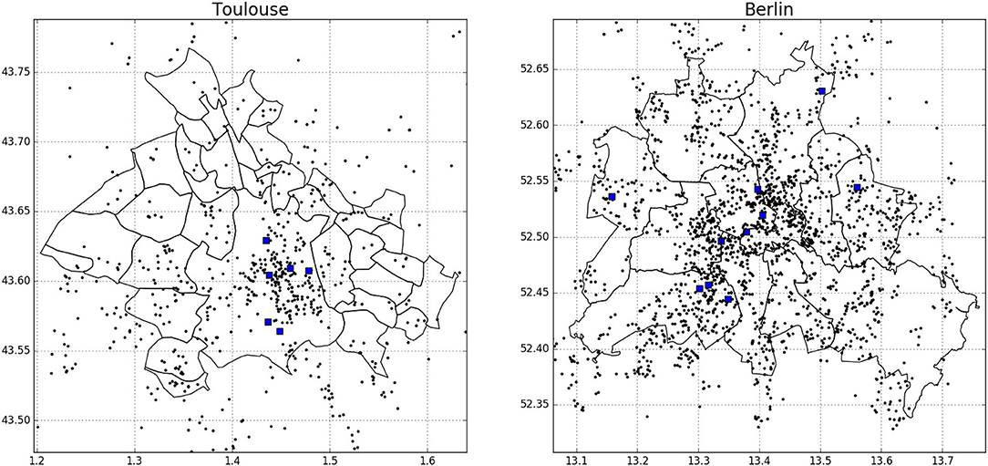
Figure 1. Maps of the two study areas, urban area of Toulouse (left) and Berlin (right). Black dots correspond to Netatmo CWS (20 June 2017, 00:00 UTC) and blue squares to reference stations. Black lines denote borders of city districts. Projection: WGS-84.
In Toulouse, the stations of a network recently set up by Météo France (Figure 1, left and Table A1 in Supplementary Material) within the city are used. Again, only stations which belong to built-up areas are used, following the LCZ classification in Hidalgo et al. (personal communication). All measurement sites consist of semi-professional Davis Vantage Pro 2 (tested in Bell et al., 2015) meteorological stations (accuracy for T ±0.5 K), equipped with actively-ventilated white radiation shields. Measurements are available at 5-min intervals and were aggregated to hourly mean values.
Netatmo Data Acquisition
Air temperature (T) data from CWS sold by the company “Netatmo” (https://www.netatmo.com/) were used in this study. An automatic work-flow was set up to fetch T data from Netatmo CWS for the investigation period, i.e., from July 1, 2016 until June 30, 2017. The setup has previously been described in Meier et al. (2017) and Fenner et al. (2017), in the following a brief summary is given. Measurements by the CWS are taken by two modules, an indoor and an outdoor module. The outdoor module measures relative humidity and T (specified accuracy ± 0.3 K in the range −40 to 65°C) at 5-min intervals, data are uploaded automatically to the Netatmo server via private Wi-Fi connection. If the user agrees, measurement data made by the outdoor module are shared online and can be obtained freely via an application programming interface (API) provided by Netatmo. The “getpublicdata” method of this API was used to obtain T data for all available CWS in Berlin and Toulouse (Figure 1) at one-hourly intervals (instantaneous values). The returned JSON objects were parsed and data written into a local MySQL database. A consistency check was carried out and all CWS that returned data with an invalid date/time were omitted. Measurements were assigned to the next full hour (e.g., all measurements between 10:00:01 h and 11:00:00 h assigned to 11:00:00 h) since the CWS do not measure at identical times. For Toulouse, data in the months July–September 2016 were acquired using the “getmeasure” method of the API. This method provides one-hourly average values for each CWS and allows the acquisition of CWS data in retrospect. One-hourly mean values differ from instantaneous values especially during the morning and afternoon hours, otherwise differences in the data obtained through the two methods are within measurement accuracy (Fenner et al., 2017). It should be noted nonetheless that CWS data are instantaneous hourly values compared to hourly mean values for the reference networks (see above). For more details concerning the CWS data acquisition the reader is referred to Meier et al. (2017). Note that the number of available CWS at each hour varies in time (Table 1), which is a unique characteristic of this data set.
Development of the QC
Before introducing the developed QC routine, the used notation is presented. The data set is represented as a matrix T ∈ (R ∪ NaN)n×m. In this matrix each row (n) contains values from one station, each column contains values from one time step (m). Not a number (NaN) is used to represent missing values or values flagged by a QC step1. If not otherwise stated, unary and binary functions containing a NaN value yield NaN. Higher order functions ignore NaN values.
Let f be a function, then f〈.〉 denotes row-wise and f〈.〉 column-wise application, i.e., parentheses refer to the temporal, and angle brackets to the spatial domain. Further, a subscript like f(.)d denotes the application for values in a given time range. The used ranges are d for days and m for month, i.e., a matrix containing the daily minima of each station could be created by min(T)d. If no range is explicitly stated, the range is hourly. As an example, a vector containing the spatial minimum for each hour would be stated as min〈T〉.
The developed QC routine consists of seven levels. The first four levels are designed to ensure the data quality and are, therefore, considered part of the main routine (M1–M4). The benefit of the following three levels (O1–O3) is dependent on the application. Therefore, those levels are considered optional. The QC-level of T is specified by an index, e.g., TM1 is a data set where QC step M1 has been applied. Each level uses the result of the previous level as input.
Main QC Levels
During level M1, the data is controlled by using the available meta data. Stations with equal longitude and latitude are set to NaN. These stations are assumed to have not been properly set up by the owner, which led to automatic location assignment based on the IP address of the wireless network (Meier et al., 2017). This is a unique feature of the Netatmo data set, but the filter could also be relevant for other CWS data sets.
In level M2 a height corrected data set () is first calculated. This is done to account for the natural vertical variation of T due to the different elevations of the CWS stations. We use globally available elevation data from the Shuttle Radar Topography Mission (SRTM), version 4.1 at 0.000833° spatial resolution (~90 m at the equator) (Jarvis et al., 2008) and extracted the nearest neighbor pixel value for each station. Let this elevation be denoted as z then is calculated as:
where 0.0065 corresponds to the usual standard atmospheric lapse rate. It should be noted that this lapse rate might not be valid in special meteorological conditions such as strong radiation inversions during night-time. The lapse-rate adjustment is an optional setting in filter step M2, which could be omitted.
This height correction has very little effect for the cities studied due to the overall relatively flat topography, but ensures the transferability of the method to other regions. As an alternative to SRTM data, the elevation information provided in the meta data of each CWS could be used in this step. However, it was decided to use SRTM data instead to ensure the transferability of the method to other crowdsourced data sets in the absence of elevation information, and since Netatmo owners can manually specify the elevation information, which could be faulty or mistaken for information regarding height above ground level. The use of SRTM data instead of the elevation provided via the API also avoided that wrong or missing elevation values reduced data availability as in Madaus et al. (2014).
Then, a modified z-score approach for outlier detection and masking of suspicious data as described in Aggarwal (2013) and Iglewicz and Hoaglin (1993) is applied. The underlying assumption of normal distribution should be given since T at a given place can be seen as a result of a large number of independent processes (central limit theorem). As recommended (Iglewicz and Hoaglin, 1993; Aggarwal, 2013; Leys et al., 2013), we use a robust method to estimate the expected value and variance of the distribution. Instead of the median absolute deviation (MAD) as estimator for variance, we use the Qn estimator established by Rousseeuw and Croux (1993), since it has been shown to be more efficient. The used implementation of Qn is from Maechler et al. (2017).
The z-score Z is calculated as:
Values that would lead to rejection of the null hypothesis for α = 0.05 on the upper tail and α = 0.01 at the lower tail of the distribution are considered faulty and therefore masked. Formally:
where i and j correspond to the time step and each of the CWS, respectively. We treat the upper tail stricter since Meier et al. (2017) showed that most common error sources in CWS data are related to indoor locations of stations or radiative errors in non-shaded areas, increasing T. It should be noted that for areas where only a small amount of CWS are available (i.e. n < 200) the use of the t-distribution for calculating the critical values would be beneficial. In section Sensitivity Tests the robustness of the QC to different cut-of values of Z is investigated.
In level M3, all data of a station within 1 month is removed if step M2 flagged more than 20% of the considered month. It is assumed that if too many values were removed by level M2, the station is too erroneous to be kept. The time frame of 1 month could be shortened if shorter time periods are to be investigated with CWS data.
Finally, in level M4, the Pearson correlation coefficient (R) between each individual station and the median of CWS is calculated for each month. If the correlation is lower than 0.9, the data in month m of the considered station j are set to NaN, such as:
The indoor stations are targeted here, since it is assumed that they are less correlated to outdoor stations as their diurnal cycles are shifted in time or otherwise non-representative of outdoor environments. The threshold of R included here will be justified in section Test 1—Indoor Stations. The application of the median is valid, as long as all stations are subject to similar meso-scale atmospheric conditions. If regions larger than a city and its surrounding areas are investigated, e.g., a whole continent, a division into sub-regions should be carried out.
Optional QC Levels
In level O1, missing values for a single time step are interpolated by the mean of the two closest values of the same station so that the time series can be as continuous as possible. These missing values are due to either server errors, failed wireless transmission, or battery failures, leading to missing data, or due to step M2 of the QC, which removed individual T values from the data set. To allow a more robust calculation of daily or monthly statistics, in levels O2 and O3 values are removed if they belong to a station with <80% data available per day and month, respectively, following the work of Meier et al. (2017).
Table 2 shows the resulting percentage of data after each steps of the QC. At each step, this percentage is similar between the two cities. Note that the steps O2 and O3 are very restrictive and decrease data availability much more than QC steps M1–M4.
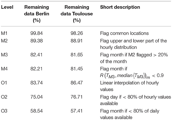
Table 2. QC steps and remaining percentage of valid data at each level.
Evaluation of the QC and Discussion
In the following, we will refer to the different data sets as: TREF for T measured by the reference stations, TRAW for raw T from CWS, TME17 when the quality control method from Meier et al. (2017) is applied to CWS data (after level D, being the highest in those procedures), and TQC when the method developed in this study is applied (after level O3). To evaluate the new QC, a qualitative evaluation is firstly carried out, followed by a comparison with the method developed by Meier et al. (2017). Then, we propose two specific tests designed to evaluate the ability of the QC to identify the indoor CWS as well as the CWS affected by radiative errors. A sensitivity analysis of the main statistical parameters in level M2 of the QC is then carried out. The evaluation is finished by quantitative comparisons between the CWS (TQC) and the reference (TREF) data sets.
Qualitative Evaluation
Time series of CWS from TQC and TRAW during January and June 2017 in Berlin are presented in Figures 2, 3, respectively. Some raw time series show a weak amplitude of diurnal cycles compared to the average (Figure 2A). They most likely belong to CWS not properly set up in an outdoor environment but rather indoors (e.g., room, basement, greenhouse) or to CWS with a dysfunction. In June, very high T (>40 °C) is also regularly measured by many CWS (Figure 3A) during daytime. These values are likely due to solar-radiation exposition, directly heating the station and leading to radiative errors (Nakamura and Mahrt, 2005). The TQC data set (Figures 2B, 3B) does not contain any CWS with very low amplitude of diurnal cycles, or stations measuring very high T. The data set is cleaned up from its outliers and the ensemble of T time series is more homogeneous, while preserving a realistic variability due to spatial heterogeneities.
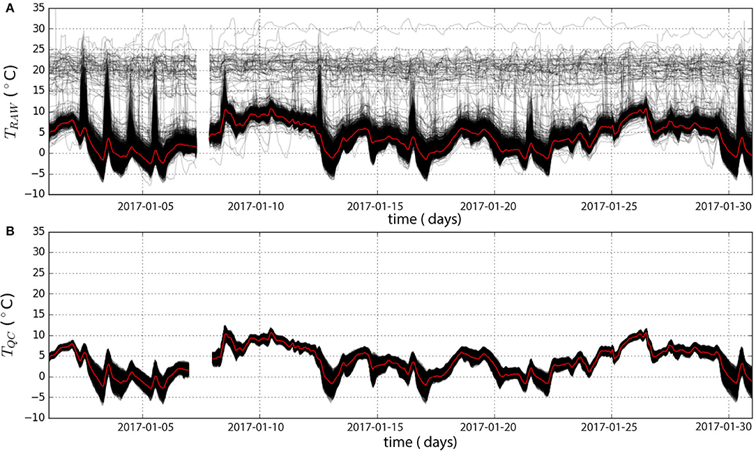
Figure 2. Temporal time series of air temperature (T) of all citizen weather stations (CWS, black) before (upper panel ≈ 1825 stations) and after (lower panel ≈ 1137 stations) the quality control (after step O3) for Berlin in January 2017. The spatial median across all CWS is shown in red.
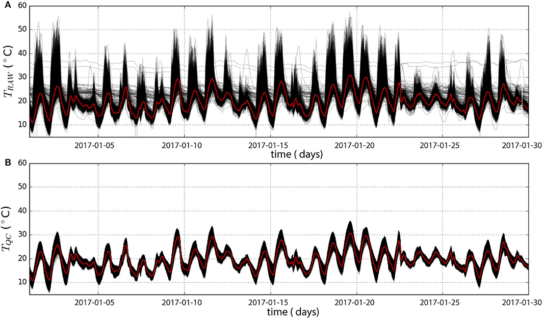
Figure 3. Same as Figure 2 but for June 2017 (upper panel ≈ 2056 stations, lower panel ≈ 1100 stations).
Looking at the spatio-temporal averages and standard deviations of the different data sets (Figure 4), it appears that the TQC data sets get closer to the TREF data set, comparing to TRAW which overestimates both the average and standard deviation of T. This can be explained by (i) the indoor stations, that are usually measuring higher T, particularly during the colder months, and (ii) the stations exposed to solar radiation, leading to unrealistically high T during daytime. As these stations are excluded in the TQC data set, the average T as well as the standard deviation decrease compared to the TRAW data set, even if they remain higher than for the TREF data set. However, differences between TREF and TRAW could also be attributed to spatial heterogeneity in T because the urban locations of both observational network are not identical.
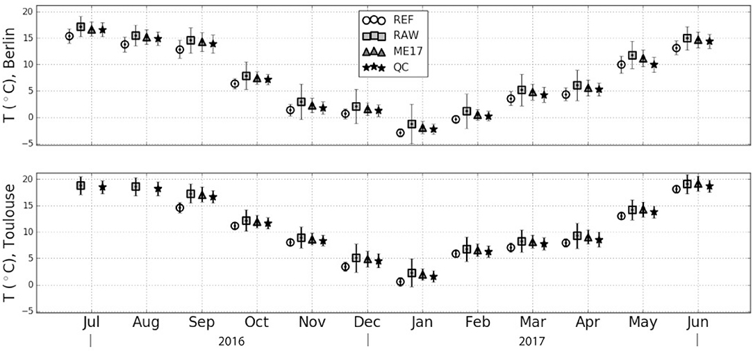
Figure 4. Spatio-temporal average and average of temporal standard deviation (in °C) of the different air temperature (T) data sets for Berlin and Toulouse per month. REF, Reference network, RAW, raw citizen weather station (CWS) data, ME17, quality-controlled CWS data according to Meier et al. (2017), QC, quality-controlled data according to this study (level O3).
Comparison to the Meier et al. (2017) Method
The spatio-temporal monthly averages and standard deviations between TME17 and TQC (Figure 4) are close in Berlin and Toulouse with a maximum difference of 0.5 K in their average and 0.3 K in their standard deviation. Compared to TME17, the TQC averages are closer to the ones calculated from the TREF data set (0.3 and 0.4 K closer on average for Berlin and Toulouse, respectively). The same improvement can be seen for the monthly standard deviation, with an average improvement of 0.1 K for Berlin and Toulouse. A positive average difference compared to the reference data set remains each month in the quality-controlled CWS data sets, also noticed by Meier et al. (2017).
However, the TQC and TME17 data sets do not resemble each other entirely. First, the ME17 approach keeps 54% of TRAW, while the new QC keeps 58% on average for Berlin and Toulouse (Table 2). Considering the total number of available raw data, 76.7% of the filter-flags are common in TME17 and TQC. Among the remaining 23.3%, there are 9.6% that correspond to T measurements which are now flagged FALSE based on the new QC. The remaining 13.7% are now flagged TRUE thereby increasing the availability of data in TQC.
These differences are mainly due to two reasons:
• The quality assessment by Meier et al. (2017) is very restrictive with the hourly daytime radiation filter [filter step C2 in Meier et al. (2017)], i.e., during daytime, T higher than three standard deviations of a set of reference stations are flagged FALSE. As shown in Figure 5a, the number of available stations strongly decreases during some specific periods of daytime, making the number of stations with valid data highly dependent on the diurnal cycle (Figure 5c). This partly explains the 13.7% of data hereafter kept in the TQC data set.
• The interpolation step (O1) of the QC increases the number of data, leading to a more continuous time series.
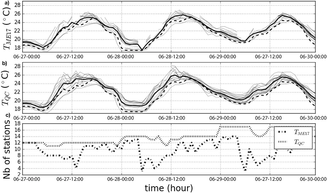
Figure 5. Air temperature (T) at citizen weather stations (CWS, gray lines) and their spatial average (thick black line) during June 27 to 29, 2017 from stations close (distance <2000 m) to the reference station Swinemuender Strasse in Berlin (thick dashed black line). (a) Applying quality control of Meier et al. (2017), (b) applying the newly developed quality control, and (c) number of CWS with valid data at each time step.
Tests
To quantitatively investigate the efficiency of the new QC, we proceed hereafter with two tests, aiming to identify whether the indoor stations and the stations exposed to shortwave (SW) radiation were properly masked from the original data set.
Test 1—indoor Stations
To investigate whether the indoor CWS, or more generally speaking the stations that were not set up properly, are flagged by the QC we calculate the Pearson correlation coefficient (R) between each individual station and the median of the reference stations for each month, using the hourly data set. Indoor stations are assumed to be less correlated to the outdoor reference stations as their diurnal cycles are shifted and altered in time.
First, this testing procedure is applied to the reference data set. All-time series of the reference data set show a correlation >0.9 with their median time series. This result justifies the threshold used in step M4 of the QC (section Development of the QC). In the following, a CWS will be considered as failing the test for 1 month if the correlation to the median of the reference stations is <0.9 with p < 0.05. For each station, a maximum of twelve tests are performed (i.e., one for each month of the year; subject to data availability). The percentage of stations failing this test in the TRAW data set is 14.6% in Berlin and 18.9% in Toulouse (Table 3). After application of the new QC the percentage of stations failing this test is 0.8% for Berlin and 2.0% for Toulouse (Table 3). This indicates that almost all stations which are not properly set up are excluded by the new QC method. This matches the qualitative result shown in Figures 2,3 for the city of Berlin.

Table 3. Percentage and number of months for the different data sets in Berlin and Toulouse which failed test 1 (c.f. section Test 1—Indoor Stations).
Test 2—Systematic Radiative Errors
To identify whether the new QC efficiently excluded the stations showing radiative errors due to solar heating, a method suggested in Meier et al. (2017) is used. For each month, the correlation between the difference of a given station to the median of the reference stations, and the SW radiation is calculated, using daytime values only, i.e., when SW > 0, (using the UCON station at the main building of the Technische Universität in Berlin and the Blagnac airport station in Toulouse). If a significant (p < 0.05) correlation is higher than 0.5 (threshold defined in Meier et al., 2017), the temporal evolution of T is considered suspicious with regard to solar radiation.
As for Test 1, the testing procedure is first applied to TREF to evaluate the test. Every station/month passes this test for Toulouse (Table 4, 0% of the months lead to correlation higher than 0.5) but not for Berlin (Table 4). Out of the 7 months failing the test, five belong to one station (Spandauer Strasse), which could be due to the micro-scale conditions around this site. Due to the site's location in a backyard behind a house and trees surrounding it, the shading conditions are highly variable along the annual and diurnal cycles. This may lead to situations when the radiation screen of the sensor is exposed to solar radiation, while the photo-voltaic panel to power the ventilation might be shaded, as it is positioned below the radiation screen. In such conditions the radiation screen would not be actively ventilated, which may lead to radiative errors (Nakamura and Mahrt, 2005). The results on the TQC and TRAW data sets are then investigated. The percentage of months during which variations of T are significantly correlated to SW radiation is 5.5% in the TQC data set, while it is 14.3% for the TRAW data set in Berlin (respectively 0.8 and 6.0% in Toulouse, Table 4).
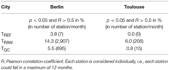
Table 4. Percentage and number of months for the different data sets in Berlin and Toulouse which failed test 2 (c.f. section Test 2—Systematic Radiative Errors).
The results for Toulouse indicate that most of the Netatmo stations that are exposed to solar radiation have been excluded from the data set by the new QC.
The two tests have shown that the quality-controlled CWS data may still contain suspicious T values. These two tests could thus be added to the entire control process if reference data sets are available (i.e., SW radiation data at one location and a sufficiently large set of T measurements from reference stations). In this study, since the aim is to develop a universally applicable technique, it was decided to not do this. These two tests could therefore be considered as optional QC steps of the whole method developed in this study and should be applied between steps O1 and O2 (section Development of the QC).
Sensitivity Tests
In the following section, the robustness of the main QC step (M2) shall be investigated. This step includes two parameters which determine the size of the removed lower and upper parts of the T distribution at each time step. These parameters are by default chosen to correspond to the value leading to rejection of the null-hypothesis for a z-test with α = 0.01 and α = 0.05 for the lower and upper part of the distribution, respectively. We test the sensitivity by making additional simulations on the data sets of Berlin and Toulouse with these parameters equal to either 50 or 150% of the default values. The two tests as described in section Tests are used to evaluate the outcome of these sensitivity tests and the results are presented in Table 5.
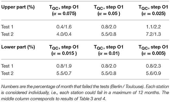
Table 5. Results of the sensitivity tests of the thresholds (upper and lower values of α) of QC step M2 for Berlin and Toulouse.
The parameter for the lower part of the distribution is very robust as the rejected percentage of data barely changes when using ± 50% of its default value (maximum 0.3% difference). For the parameter of the upper part, despite being more sensitive, the percentages of data that failed tests 1 and 2 remain close to the ones obtained with the default TQC data set with a maximum of 1.7% difference in Berlin when testing upper α = 0.025. Overall, it indicates a robustness of the method to the applied parameters.
Comparison with Reference Stations
While Figure 5b shows that T measured by the reference station is quite similar to the average of the nearby (<2,000 m) CWS, it also shows that individual CWS display larger deviations of up to 4 K. The yet unsolved challenge is to determine whether these deviations are natural or artificial. Artificial errors could be due to multiple reasons, e.g., the distance between CWS stations and building walls, station height or exposure, or close-by artificial heat sources such as exhausts or air conditioning outlets. Thus, picking somewhat randomly a pair of CWS as it is traditionally done to measure the urban heat island (UHI) (e.g., Wilby, 2003) could lead to a mis-quantification and neglects the spatial heterogeneity of T in urban regions. De Vos et al. (2017) showed that for precipitation measurements from Netatmo stations, averaging multiple stations is needed to better represent the precipitation in Amsterdam, the Netherlands, in comparison to a reference gauge-adjusted radar. Chapman et al. (2017) and Fenner et al. (2017) also pointed out some issues when considering only one CWS. Hence, we consider that data from one single station should be evaluated carefully and that a spatial average of stations should better be exploited.
Figures 6, 7 thus show a comparison between two reference stations (Berlin: Swinemuender Strasse, Toulouse: Marengo) and the weighted average of the surrounding CWS within a radius of 2,000 m (weighting is attributed using the inverse distance method, formula in Appendix A.2 in Supplementary Material). Figures 6a, 7a show scatter plots using hourly data. On average for all stations, the CWS present a positive mean deviation (MD, Appendix A.3 in Supplementary Material) with regard to the reference station of 0.95 and 0.49 K in Berlin and Toulouse, respectively (Table 6). The resulting root-mean-square deviation (RMSD) is quite low for both cities (< 1.5 K). Figures 6c, 7c show the results using daily minimum T, highlighting a stronger positive MD. This also results in a higher RMSD of 1.59 and 1.77 K for Berlin and Toulouse, respectively (Table 6). For daily maximum T, the MD is less consistent between the two cities, with an average of 0.60 K for Berlin and −0.22 K for Toulouse, resulting in relatively low RMSD (1.17 and 1.23 K). It is remarkable that an underestimation in Toulouse is found for daily maximum T (Figure 7d).
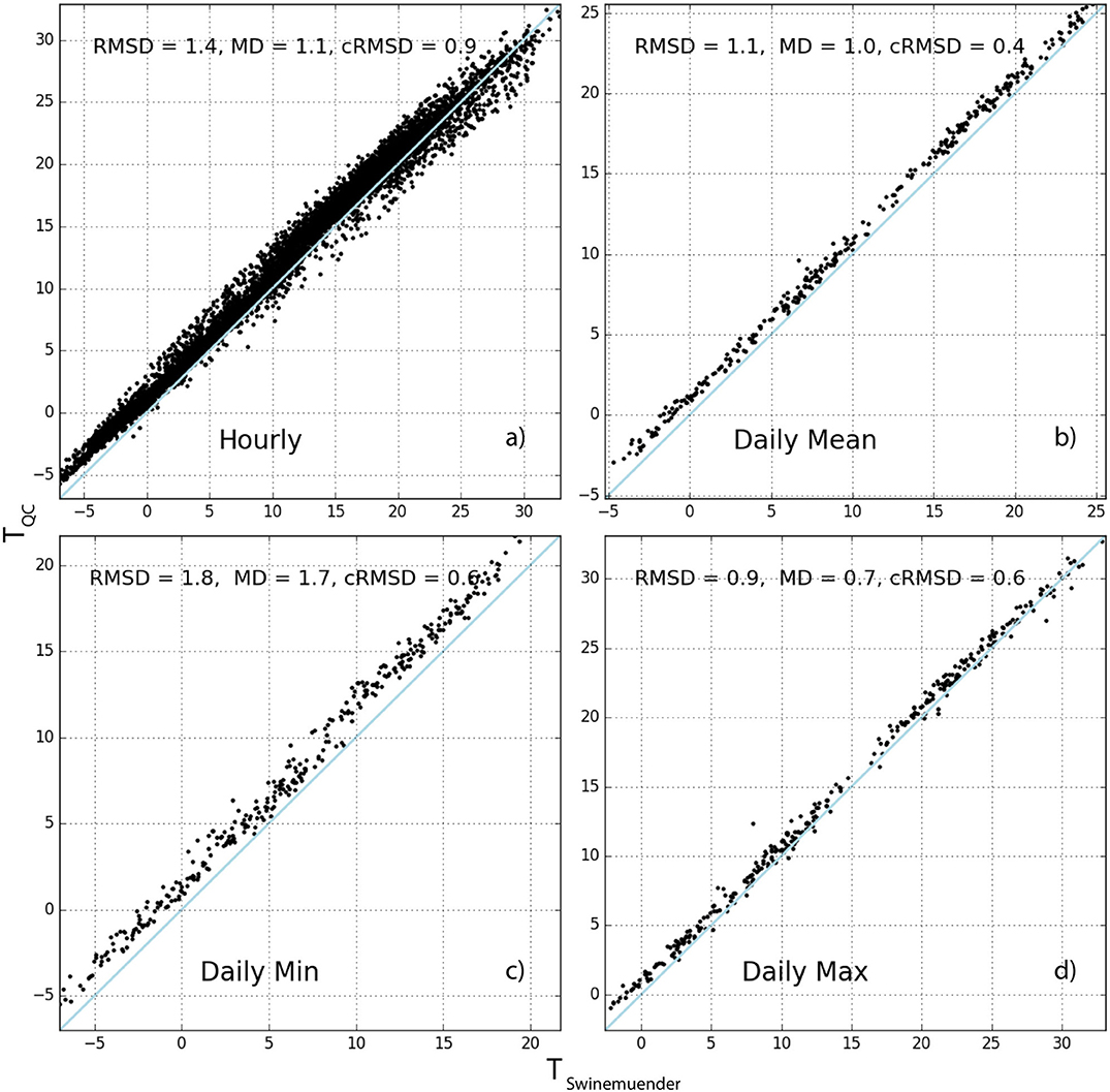
Figure 6. Relations of air temperature (T) at reference station Swinemuender Strasse in Berlin and the inverse-distance weighted average of quality-controlled T measured by citizen weather stations (TQC) within a radius of 2000 m: hourly values (a), daily mean (b), daily minimum (c), and daily maximum (d). The root-mean-square deviation (RMSD), mean deviation (MD) and centered RMSD (cRMSD) (section Appendix A.3 in Supplementary Material) are given in each panel (units K). The blue line indicates the 1:1 line.
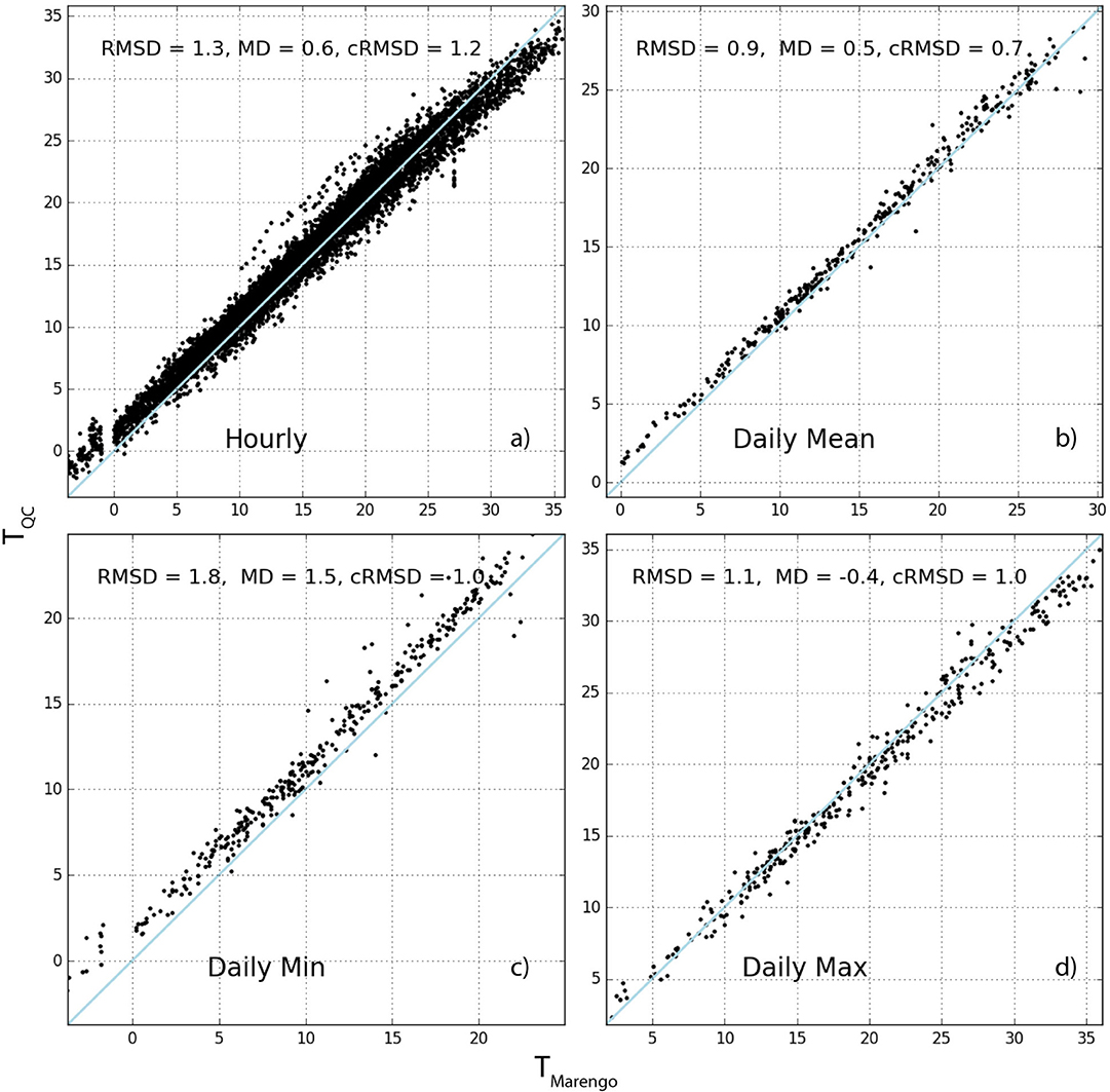
Figure 7. Same as Figure 6 but for the Marengo (Toulouse) reference station.
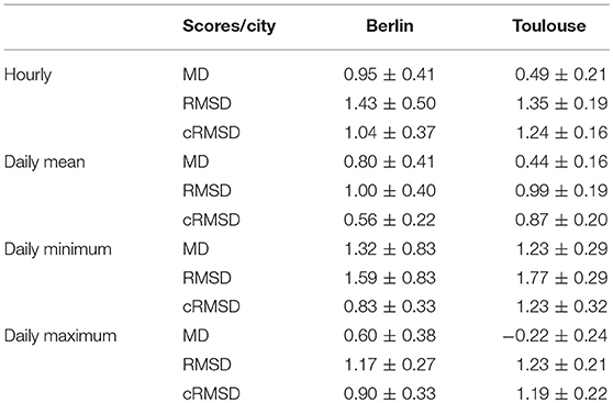
Table 6. Annual average ± standard deviation of scores (MD, RMSD, cRMSD in K, see Appendix A.3 in Supplementary Material for formula) calculated between each reference station (Berlin: ten stations, Toulouse: six stations) and the inverse-distance weighted average of the Netatmo CWS within a radius of 2,000 m.
Such positive MD were also observed in the study of Chapman et al. (2017). They showed that the deviation between CWS and a reference station fluctuates and notably increases with atmospheric stability. They assumed that this MD could be due to the fact that their reference data were more likely to be located in areas of green space. In this study, however, only reference stations that belong to non-green areas are considered. The results of Table 6 point out that this MD issue thus cannot only be explained by the difference in local-scale settings, adding to results by Fenner et al. (2017) who showed positive deviations between CWS and reference data for different LCZ classes. Further, the study of Meier et al. (2017) showed that the MD in crowdsourced T is unlikely due to instrumentation but to the siting of the station. Indeed, we assume that most of the CWS are set up close to building walls (e.g., directly on a window sill or on a balcony), especially in dense urban areas. On the contrary, the reference stations are often set up on public furniture (e.g., street lamp-posts), which are more distant to walls. Adding the fact that the Netatmo CWS do not include a proper radiation shield, we hypothesize that the observed positive MD could be due to long-wave radiation emitted by walls. This would then lead to warming of the nearby air and the aluminum casing of the Netatmo CWS. This issue of the siting of a CWS was addressed in the study of Wolters and Brandsma (2012), who excluded all CWS in their data set that were positioned too close to a building wall (<1.5 m). However, such a removal of stations is not possible with crowdsourced Netatmo data, since the meta data provided with the actual data are sparse, and do not include information about the specific set-up, as in the data set of Wolters and Brandsma (2012). These missing meta data is yet one of the biggest challenge when working with crowdsourced atmospheric data (Chapman et al., 2017).
One of the challenges of this study is to determine if the crowdsourced data set can actually represent the urban heterogeneities in surface properties and the resulting T pattern. As seen in this section, a MD is almost constantly observed between the CWS and the reference network, particularly with daily minimum T. For this reason, it is challenging to demonstrate that the CWS network is able to capture the natural spatial variation caused by local- and meso-scale forcings. In order to consider this systematic deviation, we analyze the centered root–mean-square deviation (cRMSD, Taylor, 2001, see Appendix A.3 in Supplementary Material for formula), which can be seen as the classical RMSD of unbiased time series or a combination of the correlation, and the standard deviation of both the CWS and reference time series.
Figure 8 shows, for each reference station, how the cRMSD calculated between daily minimum T of each single CWS and the reference station evolves with distance. In every case except reference station Albrechtstrasse, cRMSD increases with distance. Note that this reference station is located close to a canal in an area of allotment gardens which may strongly influence T, especially in the evening and at night (Heusinkveld et al., 2014; Steeneveld et al., 2014).
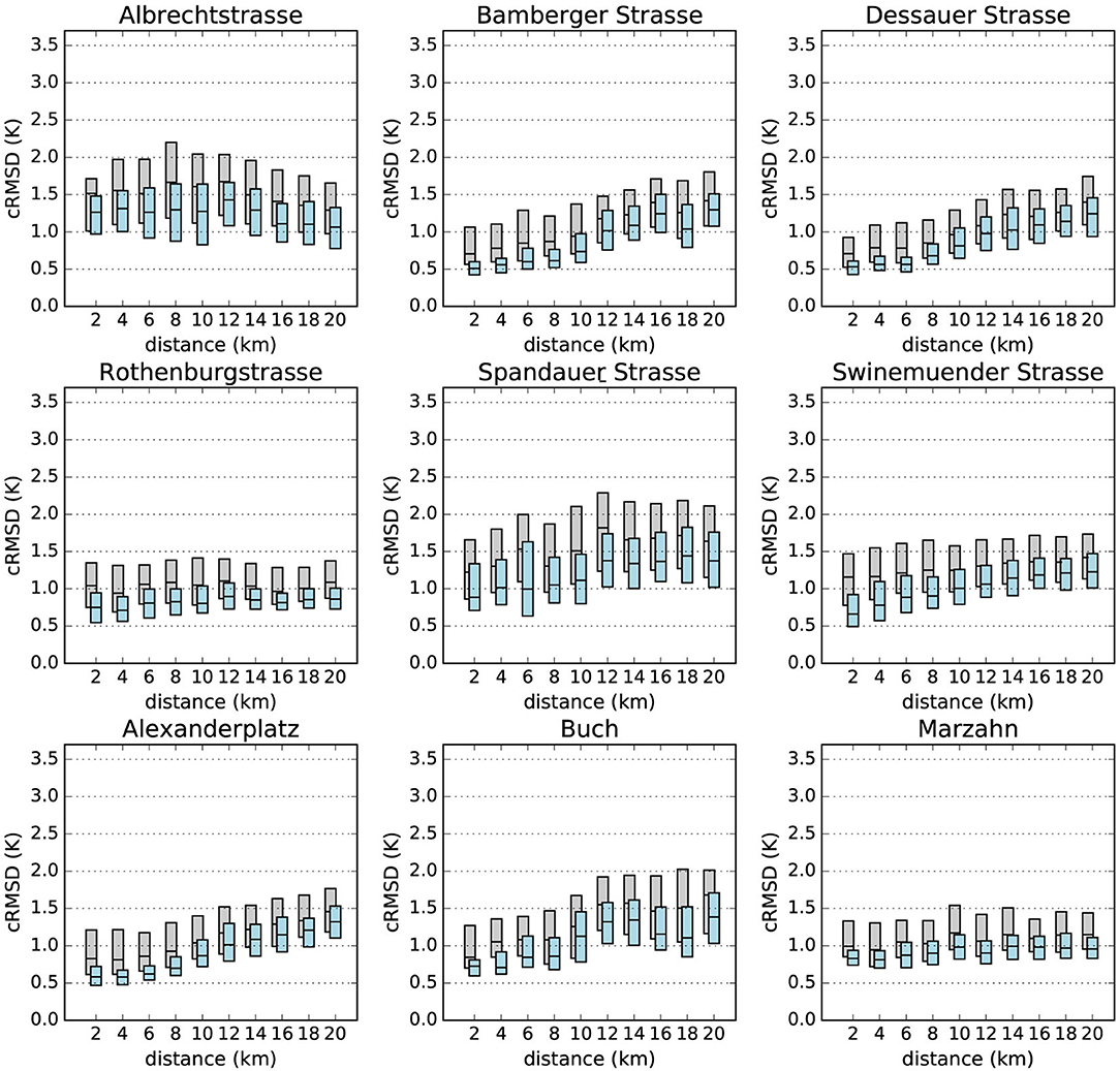
Figure 8. Boxplots of centered root-mean-square deviation (cRMSD) using daily minimum T (y axis, see Appendix 2 in Supplementary Material for definition) calculated between each individual CWS and reference stations according to the distance between them (x axis) for the investigation period July 2016 – June 2017. Scores are calculated from raw data (TRAW, gray) and after the quality control (TQC, level O3, blue). For more readability, only the 25, 50, and 75 percentiles are represented by the boxes.
The calculated cRMSD from the TRAW data set is also shown in Figure 8. Not only are the cRMSD values much higher without the QC, but the consistency between close-by CWS and reference stations is also less visible. This illustrates again the need for having an effective QC before starting any analysis.
The same spatial comparison was also performed using daily maximum T (Figure 9), showing that no clear relationship can be established for cRMSD values and the distance between individual CWS and reference stations. This can be expected since spatial T differences within a city are only weakly pronounced during daytime due to an unstable stratification of the urban atmosphere, when daily maximum T typically occurs (e.g., Fenner et al., 2017). The average cRMSD slightly varies around 1 K, independent of the distance to the reference station. Yet, the cRMSD is also greatly improved after the QC is applied.
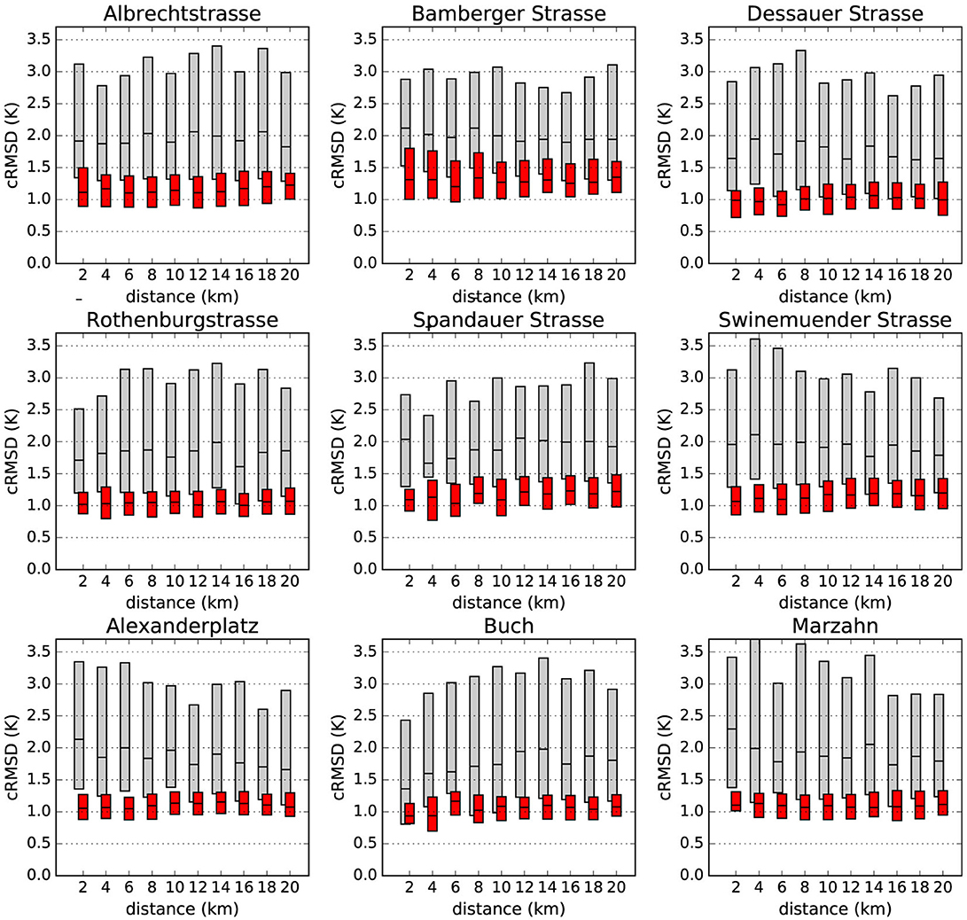
Figure 9. Same as Figure 8 but using daily maximum T. TRAW data are in gray and TQC in red.
Application
To illustrate the transferability and applicability of the newly developed QC, we apply it to crowdsourced T data observed by CWS in Paris and surrounding areas, where dense reference networks are missing and where the spatial density of Netatmo CWS is especially high. CWS data for Paris were acquired as explained in section Netatmo Data Acquisition.
We propose a spatial interpolation of T which could overcome challenges typically associated with the investigation and quantification of UHI. This method avoids (i) the spatial issues that are involved if only a single pair of stations is used (e.g., Wilby, 2003) thanks to a spatial continuum, as well as (ii) the temporal inconsistency of T measurements that are inherent in mobile transect methods (e.g., mobile measurements, Brandsma and Wolters, 2012; Leconte et al., 2015).
Figure 10 shows the estimated spatial distribution of T over Paris on 21 June 2017 at 00:00 UTC. Within the region of interest 3931 CWS are available and considered valid (at level O1) at this date and time. The T distribution is shown for a grid with 500 × 500 m spatial resolution. In each grid cell the mean T of all CWS within a radius of 2,000 m, weighted by the inverse distance method (see Appendix A.2 in Supplementary Material for formula), is shown. This radius is chosen consistently with results of section Comparison With Reference Stations and increases the number of considered stations when calculating the mean per grid cell, thus decreasing the weight of each single one of them. To strengthen this point, a value is only assigned to each grid cell if at least five CWS provide valid data. Two transects (horizontal and vertical) are also plotted in Figure 10. Note that map and transects show the differences between T and the minimum T of the whole area.
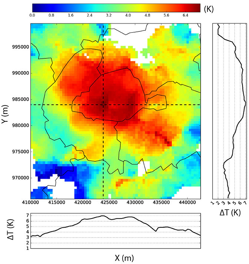
Figure 10. Spatial distribution (see text for explanations) of air temperature difference (ΔTQC) in Paris, France based on quality-controlled citizen weather station data (level O1) in Paris, June 21, 2017 at 00:00 h (UTC). ΔTQC is calculated as the difference between each individual grid box and the minimum value of the area. Dashed lines represent exemplary transects through the study region. Solid lines denote the departmental borders. Projection: Lambert conformal conic.
Figure 10 clearly indicates a spatial T pattern with higher T within the city center of Paris and lower T in the outskirts. Moreover, an inner-city differentiation of T can be seen, highlighting the possibility to obtain spatially continuous T information from CWS data that is seldom achievable with reference networks due to limited number of stations.
Conclusion and Outlook
In this study we developed a QC procedure to automatically filter out potentially erroneous data from crowdsourced T measured by CWS. Even though the QC is statistically based, it addresses common error sources in crowdsourced T data as identified by previous works (Chapman et al., 2017; Meier et al., 2017) and effectively filters out data that are affected by such errors. Moreover, the QC does not need reference data from professionally operated weather stations but uses information from the crowdsourced data set itself. It is easily transferable to other urban regions. Thus, it provides a homogeneous data set that can be used for further analyses.
Small deviations between quality controlled CWS and reference data were found when considering the spatial average of CWS in close proximity to a reference station. However, single stations show considerable larger errors, highlighting the fact that analyses relying on data from single CWS are to be treated carefully. A positive MD remained in the quality-controlled CWS data set, notably for daily minimum T. This issue is likely related to the siting of the CWS (i.e., close to walls) compared to the siting of standard meteorological observations at urban sites and could be investigated in detail in a future study. Despite the positive deviation, CWS data provide valuable information of T by capturing local-scale variations. These evaluations permit to justify the construction of a T map in the city of Paris using direct measurements.
Apart from the positive MD mentioned above, it could be investigated in more detail whether or not CWS data are able to capture hot or cold spots in urban areas at a finer spatial scale (i.e., <1 km) related to the underlying surface properties (e.g., sky view factor, water surface fraction, vegetation height). High resolution professional data sets are necessary for this investigation too, as well as accurate knowledge of the land cover and more detailed meta data about the CWS (i.e. orientation, height). In a further study, the applicability of the new QC for atmospheric humidity, precipitation, and wind speed and direction could be investigated.
Code Availability
Example data and the code used to perform the QC described in this work is publicly available as an R-package at the DepositOnce service of the Technische Universität Berlin under https://doi.org/10.14279/depositonce-6740.3.
Author Contributions
All authors contributed to the design and implementation of the research. AN and TG carried out the coding, calculations, and analyses. AN wrote the manuscript with support from TG, FM, and DF. TG, FM, and DF performed the collection and processing of crowdsourced data for Berlin, Toulouse, and Paris. DF collected and processed reference data for Berlin. AN collected and processed reference data for Toulouse.
Conflict of Interest Statement
The authors declare that the research was conducted in the absence of any commercial or financial relationships that could be construed as a potential conflict of interest.
Acknowledgments
The authors thank the owners of the Netatmo stations who shared their data. They also thank Guillaume Poujol from CNRM, and Hartmut Küster and Ingo Suchland from the Chair of Climatology for setting up and maintaining the professional weather station networks in Toulouse and Berlin, respectively, funded by the CNRM and Toulouse Métropole and the Technische Universität Berlin, respectively. DF is funded by the Deutsche Forschungsgemeinschaft (DFG) as part of the research project ‘Heat waves in Berlin, Germany–urban climate modifications’ (Grant No. SCHE 750/15-1). TG is funded by the German Ministry of Research and Education as part of the research programme ‘Urban Climate Under Change ([UC]2)’ (funding code: 01LP1602A).
Supplementary Material
The Supplementary Material for this article can be found online at: https://www.frontiersin.org/articles/10.3389/feart.2018.00118/full#supplementary-material
Footnotes
1. ^1In the code implementation these two cases are treated differently. Quality-controlled values are marked by a flag instead of setting them to NaN. However, the implementation details are omitted in the text here to allow a better understanding of the main ideas.
References
Aggarwal, C. C. (2013). “High-dimensional outlier detection: the subspace method,” in Outlier Analysis (New York, NY: Springer), 135–167.
Bell, S., Cornford, D., and Bastin, L. (2013). The state of automated amateur weather observations. Weather 68, 36–41. doi: 10.1002/wea.1980
Bell, S., Cornford, D., and Bastin, L. (2015). How good are citizen weather stations? Addressing a biased opinion. Weather 70, 75–84. doi: 10.1002/wea.2316
Brandsma, T., and Wolters, D. (2012). Measurement and statistical modeling of the urban heat island of the city of Utrecht (the Netherlands). J. Appl. Meteorol. Climatol. 51, 1046–1060.
Chapman, L., Bell, C., and Bell, S. (2017). Can the crowdsourcing data paradigm take atmospheric science to a new level? A case study of the urban heat island of London quantified using Netatmo weather stations. Int. J. Climatol. 37, 3597–3605. doi: 10.1002/joc.4940
Chapman, L., Muller, C. L., Young, D. T., Warren, E. L., Grimmond, C. S. B., Cai, X.-M., et al. (2015). The Birmingham urban climate laboratory: an open meteorological test bed and challenges of the smart city. Bull. Am. Meteorol. Soc. 96, 1545–1156. doi: 10.1175/BAMS-D-13-00193.1
Cook, C. (2011). Grassroots clinical research using crowdsourcing. J. Man. Manip. Ther. 19, 125–126. doi: 10.1179/106698111x12998437860767
De Vos, L., Leijnse, H., Overeem, A., and Uijlenhoet, R. (2017). The potential of urban rainfall monitoring with crowdsourced automatic weather stations in Amsterdam. Hydrol. Earth Syst. Sci. 21, 765–777. doi: 10.5194/hess-21-765-2017
Dickinson, J. L., Zuckerberg, B., and Bonter, D. N. (2010). Citizen science as an ecological research tool: challenges and benefits. Annu. Rev. Ecol. Evol. Syst. 41, 149–172. doi: 10.1146/annurev-ecolsys-102209-144636
Droste, A. M., Pape, J. J., Overeem, A., Leijnse, H., Steeneveld, G.-J., and Uijlenhoet, R. (2017). Crowdsourcing urban air temperatures through smartphone battery temperatures in São Paulo, Brazil. J. Atmos. Oceanic Technol. 34, 1853–1866. doi: 10.1175/jtech-d-16-0150.1
DWD Climate Data Center (CDC) (2017). Historical Hourly Station Observations of 2m Air Temperature and Humidity – Version v005.
Fenner, D., Meier, F., Bechtel, B., Otto, M., and Scherer, D. (2017). Intra and inter 'local climate zone' variability of air temperature as observed by crowdsourced citizen weather stations in Berlin, Germany. Meteorol. Z. 26, 525–547. doi: 10.1127/metz/2017/0861
Fenner, D., Meier, F., Scherer, D., and Polze, A. (2014). Spatial and temporal air temperature variability in Berlin, Germany, during the years 2001–2010. Urban Clim. 10, 308–331. doi: 10.1016/j.uclim.2014.02.004
Hammerberg, K., Brousse, O., Martilli, A., and Mahdavi, A. (2018). Implications of employing detailed urban canopy parameters for mesoscale climate modelling: a comparison between WUDAPT and GIS databases over Vienna, Austria. Int. J. Climatol. 38, e1241–e1257. doi: 10.1002/joc.5447
Heusinkveld, B. G., Steeneveld, G. J., van Hove, L. W. A., Jacobs, C. M. J., and Holtslag, A. A. M. (2014). Spatial variability of the Rotterdam urban heat island as influenced by urban land use. J. Geophys.Res. 119, 677–692. doi: 10.1002/2012jd019399
Iglewicz, B. and Hoaglin, D. C. (1993). How to detect and handle outliers, Vol. 16. Milwaukee, WI: ASQC Quality Press
Jarvis, A., Reuter, H. I., Nelson, A., and Guevara, E. (2008). Hole-Filled Seamless SRTM data V4, International Centre for Tropical Agriculture (CIAT). Available online at: http://srtm.csi.cgiar.org
Kaspar, F., Müller-Westermeier, G., Penda, E., Mächel, H., Zimmermann, K., Kaiser-Weiss, A., et al. (2013). Monitoring of climate change in Germany–data, products and services of Germany's National Climate Data Centre. Adv. Sci. Res. 10, 99–106. doi: 10.5194/asr-10-99-2013
Kim, Y. H., Ha, J. H., Yoon, Y., Kim, N. Y., Hyucim, H., Sim, S., et al. (2016). Improved correction of atmospheric pressure data obtained by smartphones through machine learning. Comput. Intell. Neurosci. 2016:9467878. doi: 10.1155/2016/9467878
Kottek, M., Grieser, J., Beck, C., Rudolf, B., and Rubel, F. (2006). World map of the Köppen-Geiger climate classification updated. Meteorol. Z. 15, 259–263. doi: 10.1127/0941-2948/2006/0130
Leconte, F., Bouyer, J., Claverie, R., and Pétrissans, M. (2015). Using Local Climate Zone scheme for UHI assessment: evaluation of the method using mobile measurements. Build. Environ. 83, 39–49. doi: 10.1016/j.buildenv.2014.05.005
Leys, C., Ley, C., Klein, O., Bernard, P., and Licata, L. (2013). Detecting outliers: do not use standard deviation around the mean, use absolute deviation around the median. J. Exp. Soc. Psychol. 49, 764–766. doi: 10.1016/j.jesp.2013.03.013
Madaus, L. E., Hakim, G. J., and Mass, C. F. (2014). Utility of dense pressure observations for improving mesoscale analyses and forecasts. Mon. Weather Rev. 142, 2398–2413. doi: 10.1175/MWR-D-13-00269.1
Maechler, M., Rousseeuw, P., Croux, C., Todorov, V., Ruckstuhl, A., Salibian-Barrera, M., et al. (2017). Package ‘robustbase.’
McNicholas, C., and Mass, C. F. (2018). Smartphone pressure collection and bias correction using machine learning. J. Atmos. Ocean. Technol. 35, 523–540. doi: 10.1175/JTECH-D-17-0096.1
Meier, F., Fenner, D., Grassmann, T., Otto, M., and Scherer, D. (2017). Crowdsourcing air temperature from citizen weather stations for urban climate research. Urban Clim. 19, 170–191. doi: 10.1016/j.uclim.2017.01.006
Muller, C., Chapman, L., Johnston, S., Kidd, C., Illingworth, S., Foody, G., et al. (2015). Crowdsourcing for climate and atmospheric sciences: current status and future potential. Int. J. Climatol. 35, 3185–3203. doi: 10.1002/joc.4210
Nakamura, R., and Mahrt, L. (2005). Air temperature measurement errors in naturally ventilated radiation shields. J. Atmos. Ocean. Technol. 22, 1046–1058. doi: 10.1175/jtech1762.1
Oke, T. R. (1982). The energetic basis of the urban heat island. Q. J. R. Meteorol. Soc. 108, 1–24. doi: 10.1002/qj.49710845502
Overeem, A. R., Robinson, J., Leijnse, H., Steeneveld, G.-J. P., Horn, B., and Uijlenhoet, R. (2013). Crowdsourcing urban air temperatures from smartphone battery temperatures. Geophys. Res. Lett. 40, 4081–4085. doi: 10.1002/grl.50786
Rousseeuw, P. J., and Croux, C. (1993). Alternatives to the median absolute deviation. J. Am. Stat. Assoc. 88, 1273–1283. doi: 10.1080/01621459.1993.10476408
Steeneveld, G., Koopmans, S., Heusinkveld, B., and Theeuwes, N. (2014). Refreshing the role of open water surfaces on mitigating the maximum urban heat island effect. Landsc. Urban Plan. 121, 92–96. doi: 10.1016/j.landurbplan.2013.09.001
Taylor, K. E. (2001). Summarizing multiple aspects of model performance in a single diagram J. Geophys. Res. 106, 7183–7192. doi: 10.1029/2000JD900719
Wilby, R. L. (2003). Past and projected trends in London's urban heat island. Weather 58, 251–260. doi: 10.1256/wea.183.02
Keywords: urban climate, crowdsourcing, citizen weather stations, air temperature, data quality, quality control
Citation: Napoly A, Grassmann T, Meier F and Fenner D (2018) Development and Application of a Statistically-Based Quality Control for Crowdsourced Air Temperature Data. Front. Earth Sci. 6:118. doi: 10.3389/feart.2018.00118
Received: 06 April 2018; Accepted: 30 July 2018;
Published: 29 August 2018.
Edited by:
Gert-Jan Steeneveld, Wageningen University & Research, NetherlandsReviewed by:
Luke Madaus, Fiske Planetarium, University of Colorado Boulder, United StatesSimon Bell, University of Birmingham, United Kingdom
Copyright © 2018 Napoly, Grassmann, Meier and Fenner. This is an open-access article distributed under the terms of the Creative Commons Attribution License (CC BY). The use, distribution or reproduction in other forums is permitted, provided the original author(s) and the copyright owner(s) are credited and that the original publication in this journal is cited, in accordance with accepted academic practice. No use, distribution or reproduction is permitted which does not comply with these terms.
*Correspondence: Adrien Napoly, YWRyLm5hcG9seUBnbWFpbC5jb20=
Fred Meier, ZnJlZC5tZWllckB0dS1iZXJsaW4uZGU=