What is the smallest physically acceptable scale for 1D turbulence schemes?

In numerical weather prediction (NWP) models, at mesoscale, the sub-grid convective boundary-layer turbulence is dominated by the uni-dimensional (1D) vertical thermal production. In Large-Eddy Simulations (LES), the thermal plumes are resolved and the residual sub-grid turbulent motions are homogeneous and isotropic, thus three-dimensional (3D), resulting from the dynamical production. This article sets the critical horizontal resolution for which the usually 1D turbulence schemes of NWP models must be replaced by 3D turbulence schemes. LES from five dry and cumulus-topped free convective boundary layers and one forced convective boundary layer are performed. From these LES data, the thermal production and vertical and horizontal dynamical productions are calculated at several resolutions from LES to mesoscale. It appears that the production terms of both dry and cumulus-topped free convective boundary layers have the same behavior. A pattern emerges whenever data are ranked by the resolution scaled by the size of thermal plumes, (h + h_c, where h is the boundary-layer height and h_c is the depth of the cloud layer). In free convective boundary layers, the critical horizontal resolution for which the horizontal motions must be represented is 0.5(h + h_c). However, the critical horizontal resolution in the forced convective boundary layer case is 3(h + h_c).

1. Introduction

Wyngaard (2004) first described the gray zone of turbulence, which he calls terra incognita. In this range of scales, the grid spacing is on the order of the dominant length scale in the atmospheric boundary layer (BL). The turbulent eddies are neither entirely sub-grid scale as at mesoscale, nor mainly resolved as in the Large-Eddy Simulations (LES). Honnert et al. (2011) studied the gray zone of turbulence in dry and cloudy free convective BLs (CBLs) using LES data. The authors showed that the gray zone of turbulence ranges from 0.2 to 2(h + h_c), where h is the boundary-layer height and h_c is the depth of the cloud layer and they proposed recommendations of the sub-grid/resolved partitioning of the turbulence. Shin and Hong (2013) extended this method to forced CBLs, where the BL is driven both by buoyancy and shear. BL thermals were thoroughly investigated in the latter two studies. At large scale, these structures produce uni-dimensional (1D) thermal turbulence, (André et al. 1978). On the other hand, in LES, the thermal production is resolved and the turbulence is homogeneous, isotropic and produced by the three-dimensional (3D) motions of eddies resulting from dynamical processes. It follows that the usually 1D turbulence schemes must be converted into 3D ones in the gray zone of turbulence. Thanks to increasing numerical resources, numerical weather prediction (NWP) models have now grid spacing of the order of 1 km. So they enter or have already entered the gray zone of turbulence. But, how does this transition proceed on production terms? When is the horizontal grid spacing no longer suitable for a 1D scheme? This article addresses these questions for free and forced CBLs.

It is organized as follows. Section 2 gives a description of the method used, followed by a presentation of LES cases from field campaigns where the simulations used are taken as that of the true atmosphere. Thence the dynamic and thermal productions of the turbulence kinetic energy (TKE) are calculated. Section 3 deals with the quantification of the dynamical and thermal production of TKE at all scales. Section 4 is dedicated to discussion.

2. Methods

High resolution fields from LES are considered as a reference accurately describing the turbulent motions. Horizontal averaging of the LES fields is used to calculate the production terms of the turbulence at coarser resolutions.

2.1. LES Cases

The free convective LES cases used in this study are taken from Honnert et al. (2011). Three cases of dry CBLs are presented. The first one, IHOP, corresponds to a clear continental growing CBL (see Couvreux et al., 2005 for details of this case). The second case, Wangara, Clarke et al. (1971) presents a growing boundary layer over Australia (without horizontal advection). The last case, AMMA, Redelsperger et al. (2006) has a heat flux twice as large as in the previous simulations. In addition, two cases of cumulus non-drizzling CBLs are used. The first case, BOMEX, presents marine shallow cumulus (Siebesma et al., 2002). The second case, ARM, presents a cumulus-topped CBL over land (Brown et al., 2002). Finally, in this study, a forced convective boundary layer, TRAC (Turbulence Radar Avion Cellules, Bernard-Trottolo et al., 2004), is added. TRAC took place in the Beauce Plain, some 80 km south-west of Paris, far away from any sea coast or mountain. The surface is flat and homogeneous, devoted to cereal-growing with no forest or large urban area. The campaign lasted from June 15th to July 5th 1998. The simulated period is June 29th from 9 to 18 LT. The LES presents mesoscale structures (convective rolls) which is consistent with $\frac{-h}{L_{MO}}=4.7$ on average (Weckwerth, 1995). All LES data are selected so that the production terms only depends on $\frac{\Delta x}{\text{h}+{\text{h}}_{\text{c}}}$, where Δx is the horizontal grid spacing (Honnert et al., 2011). A summary of the case properties is listed in Table 1.

TABLE 1

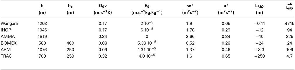
Table 1. Modeled boundary-layer characteristics (mean values over the used periods) : boundary-layer height (h), depth of the cloud layer (h_c) when there are clouds (criteria : condensed water mixing ratio larger than 10⁻⁶kg.kg⁻¹), surface buoyancy flux (Q₀v), surface humidity flux (E₀), convective vertical velocity (w*), friction velocity (u*), Monin-Obukhov length (L_MO) and $\frac{-\text{h}}{L_{MO}}$.

The Meso-NH model (Lafore et al., 1998) is used to conduct LES of the six flat diurnal cases. The five free CBLs are performed on a 16 × 16 × 5 km³ domain, whereas the forced CBL is performed on a 32 × 32 × 6 km³ domain. The horizontal grid size is 62.5 m. The vertical resolution increases when nearing the ground. The stetching depends on simulated cases but the vertical grid spacing is always less than 100 m in the boundary layer, so that the grid boxes are close to cubic in the BL. A summary of the simulation properties is listed in Table 2.

TABLE 2

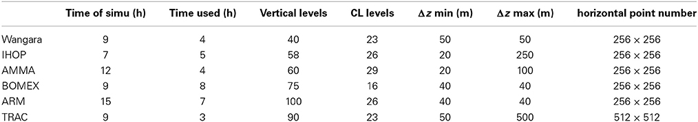
Table 2. Summary of the LES : simulation time, used time in the diagnostics, number of vertical points, number of points in the BL, vertical finest resolution, vertical coarsest resolution, number of horizontal points.

2.2. Mean Operator

The resulting LES fields are considered as the “truth.” The resolved fields at coarser resolutions are calculated by horizontally averaging the following parameters, viz the wind components and virtual potential temperature (see Honnert et al., 2011), as shown in Figure 1. This method produces a^Δx, the average value of a (a, a field at random) over a Δx scale. a^Δx is the “true” resolved value of a at a Δx grid spacing.

FIGURE 1

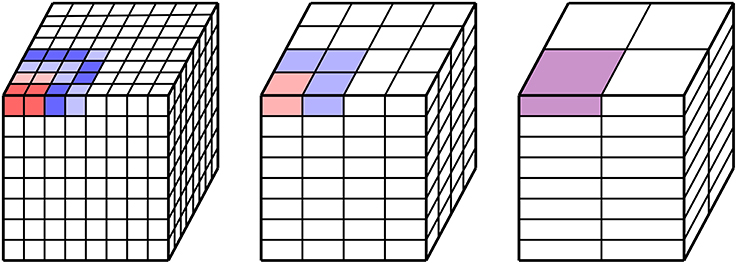
Figure 1. Illustration of the approach : successive means at different scales for Δx equal to the LES mesh size, Δx equal to two times the LES mesh size and Δx equal to four times the LES mesh size.

2.3. Computation of the Production Terms

The prognostic equation of the sub-grid TKE is:

$\begin{array}{l}\underset{\text{Tendency}}{\underbrace{\frac{\partial \overline{e}}{\partial t}}}=\underset{\text{Advection}}{\underbrace{-\overline{u_i}\frac{\partial \overline{e}}{\partial x_i}}}\underset{\begin{array}{l}\text{Turbulent}\\ \text{transport}\end{array}}{\underbrace{-\frac{\partial (\overline{{u^{\prime }}_i{e}^{\prime }}+\overline{{u^{\prime }}_i{p}^{\prime }})}{\partial x_i}}}\underset{\begin{array}{l}\text{Dynamical}\\ \text{production}\end{array}}{\underbrace{-\overline{{u^{\prime }}_i{u^{\prime }}_j}\frac{\partial \overline{u_j}}{\partial x_i}}}+\underset{\begin{array}{l}\text{Thermal}\\ \text{production}\end{array}}{\underbrace{\beta \overline{{u^{\prime }}_3{{\theta }^{\prime }}_v}}}\\ -\underset{\text{Dissipation}}{\underbrace{\nu \overline{\frac{\partial {u^{\prime }}_i}{\partial x_j}\frac{\partial {u^{\prime }}_i}{\partial x_j}}}}\end{array}$

where e is the TKE, p the pressure, θ_v is the virtual potential temperature, β the buoyancy parameter, ν the viscosity. u_i is a wind velocity component, i and j are between 1 and 3, u₃ is the vertical velocity. a is the resolved part of a and a′ = a − a is the sub-grid a. This equation respects the Einstein notation.

In this equation, the TKE locally varies because of the transport terms (advection, turbulent transport and fluctuation of pressure), the production terms, due to the shear (dynamical production) and the buoyancy (thermal production), and the dissipation of the energy (conversion of kinetic energy into internal energy). The dynamical production terms are 3D, while the thermal production term is 1D (vertical). The question is whether the horizontal dynamical production terms are negligeable at a given grid spacing Δx.

The sub-grid thermal production term at a Δx grid spacing is:

$<\beta {\overline{(u_3-{\overline{u_3}}^{\Delta x})({\theta }_v-{\overline{{\theta }_v}}^{\Delta x})}}^{\Delta x}>$

where < a > is the average value of a over the whole domain at a given altitude, which is independent of the grid size.

The dynamical production term at a Δx grid spacing is :

$<{\overline{(u_i-{\overline{u_i}}^{\Delta x})(u_j-{\overline{u_j}}^{\Delta x})}}^{\Delta x}\frac{\partial {\overline{u_i}}^{\Delta x}}{\partial x_j}>$

where ${\overline{(u_i-{\overline{u_i}}^{\Delta x})(u_j-{\overline{u_j}}^{\Delta x})}}^{\Delta x}$ is the sub-grid flux of the wind component u_j in the i direction.

3. Results

In this section, the production terms are calculated at several resolutions using the above method. As structures are more organized (mesoscale rolls) in the forced CBL, the resolved part of the turbulence is larger than in free CBLs for the same $\frac{\Delta x}{\text{h}+{\text{h}}_{\text{c}}}$ (Shin and Hong, 2013). That is why the results from free and forced CBLs are analyzed separately. The resolved and sub-grid parts of the turbulence in free CBLs only depend on $\frac{\Delta x}{\text{h}+{\text{h}}_{\text{c}}}$ (Honnert et al., 2011). It follows that the production terms are represented as a function of $\frac{\Delta x}{\text{h}+{\text{h}}_{\text{c}}}$.

3.1. Turbulence Production in Free CBLs

The ratio of the horizontal and vertical dynamical productions, as well as the thermal production, to the total production at several grid spacings can be seen on Figure 2A for the five free CBL cases. The data are inside the boundary layer.

FIGURE 2

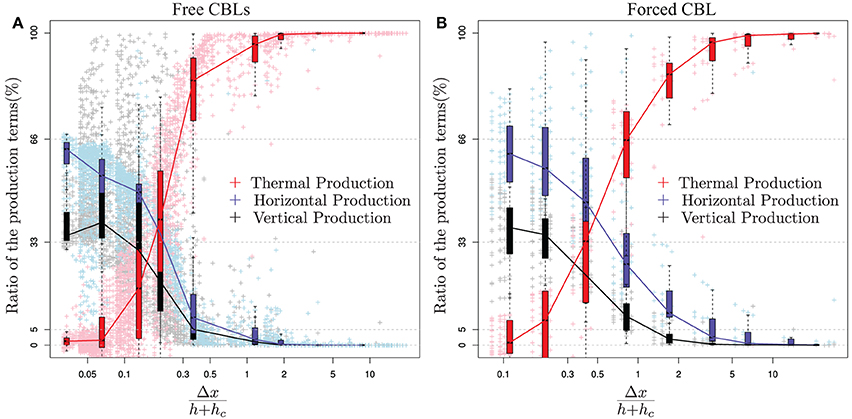
Figure 2. Ratio of the thermal production (in red), the horizontal dynamical production (in blue) and the vertical dynamical production (in black) out of the total production as a function of $\frac{\Delta x}{\text{h}+{\text{h}}_{\text{c}}}$ for (A) the simulations IHOP, AMMA, Wangara, ARM and BOMEX, and (B) TRAC.

First of all, the five simulations lie on top of each other. Hence, the assumption that the sub-grid ratio of production terms only depend on $\frac{\Delta x}{\text{h}+{\text{h}}_{\text{c}}}$ is true. For the finest grid spacing, the thermal production is null as the thermal plumes are entirely resolved. The turbulence production is entirely dynamical and the horizontal production is about two-thirds of the total production. Indeed, the sub-grid turbulence is fully isotropic in the mixed layer (500 m altitude) in the LES. The turbulence from the surface BLs and the entrainment zones are not. That is why the horizontal production is less than two-thirds and the vertical production is more than one-third on Figure 2A. When the grid spacing becomes coarser, the thermal production part grows while both the vertical and horizontal production terms decrease as the thermal plumes become subgrid. A term is considered negligible when it represents less than 5% of the total motions. The finer scale in free CBLs where the horizontal motions can be ignored is 0.5(h + h_c). In BLs of mid-latitudes, where the BL is about 1000 m depth, the critical grid spacing would be 500 m.

Beare (2014) defined the gray zone from the dissipation length scale rather than from the grid spacing of the model. This underlies the fact that the sub-grid part of a turbulent scheme not only depends on the grid spacing of the model, but also on the dissipation of a model. This implies that the critical length Δx calculated here must be understood as an effective resolution Skamarock (2003), when used in a model.

Moreover, Figure 2A shows that in the gray zone the turbulence is not fully isotropic. Firstly, the thermals are not completely resolved, thus the vertical component of the sub-grid thermal mixing must be represented by an updraft. Secondly, the components of the dynamical turbulence are not equal, as the vertical component is stronger than each of the horizontal terms. Indeed, the vertical dynamical production represents more than half of the horizontal dynamical production.

3.2. Turbulence Production in a Forced CBL

By definition, in a forced CBL, the sub-grid dynamical production is important as the wind strongly mixes the boundary layer. Figure 2B is similar to Figure 2A but applied to the TRAC LES. For the finer resolutions, the coarser eddies are resolved as in a free CBL. However, in TRAC, mesoscale structures (convective rolls) are present. As these structures are large, they are completely resolved at resolutions coarser than 0.1(h + h_c), whereas at this resolution the convective structures are partly sub-grid in free CBLs. When the resolution becomes coarser, the decrease of the dynamical production is slower than in free BLs. The finer scale in forced convective boundary layers for which the horizontal motions can be ignored is 3(h + h_c), about 2.3 km resolution in the case of TRAC, where the BL height is about 760 m (at 14 h LT).

4. Discussion

This article provides recommendations about the dimensionality of a turbulence scheme when used in convective cases in the gray zone of turbulence. The dimensionality depends on the wind shear (forced or free CBLs) and on the resolution normalized by the boundary-layer height together with the depth of the cloud layer ($\frac{\Delta x}{\text{h}+{\text{h}}_{\text{c}}}$). In free CBLs, the dimensionality of the scheme must be 3D if $\frac{\Delta x}{\text{h}+{\text{h}}_{\text{c}}}$ ≤ 0.5. In forced CBLs, the dimensionality of the scheme must be 3D if $\frac{\Delta x}{\text{h}+{\text{h}}_{\text{c}}}$ ≤ 3. The transition between free and forced BLs is not addressed in this article. The difference in behavior between the free BLs and TRAC is the presence of mesoscale structures.

Some recent studies have shown that models need to be improved to run in the gray zone of turbulence. Wyngaard (2004) studied the transport of scalars in the surface boundary layer using observational data. He found out that the production terms in the gray zone of turbulence should be represented by tensor eddy-diffusivity. Hatlee and Wyngaard (2007) extended this study to advection, vertical turbulent transport and buoyant production terms. It is well-known that the eddy-diffusivity approach alone cannot adequately represent the upper part of the CBL. The non-local turbulence has to be represented at mesoscale, as well as in the gray zone. However, Honnert et al. (2011) showed that in free CBLs the non-local mixing has to be reduced when the resolution enters the gray zone of turbulence while the local mixing can remain unchanged. The authors proposed to used the two-scale separation of Eddy-diffusivity/Mass-flux (EDMF) schemes (Hourdin et al., 2002; Soares et al., 2004). Indeed, in EDMF schemes, the mass-flux parametrization represents the non-local buoyancy production while the local dynamical production is represented by the eddy-diffusivity part. Likewise, in Arakawa et al. (2011) and Arakawa and Wu (2013), the author modified the mass-flux deep convection scheme and increased the updraft fraction so that the parametrization can be adapted to the gray zone of convection. Some other schemes are developed to overcome the limitations in the gray zone. Dorrestijn et al. (2013) made a stochastic parametrization based on LES data of a convective boundary layer. Using the law of Honnert et al. (2011), Boutle et al. (2014) blended a mesoscale parametrization and a LES turbulence scheme to generate a partially-resolved turbulence parametrization.

However, although the gray zone of turbulence is at first reached by the convective structures, this study shows that 3D dynamical movements are necessary in turbulence schemes in the gray zone. The horizontal movements of the non-local structures are not always taken into account in the schemes, and these modifications may be difficult to implement in NWP models. For example, as the AROME model has only 1D parametrizations, the implementation of a 3D turbulence scheme would require a complete reorganization of the code.

Finally, when the horizontal turbulence is taken into account, for instance, in Boutle et al. (2014), it is assumed isotropic. This study shows that the shear-driven turbulence is not isotropic in the gray zone. Thus, a scale adaptive turbulent scheme must have different eddy diffusivities on the horizontal and on the vertical, which is not the case when LES schemes, such as the Smagorinsky-type schemes, are used.

Conflict of Interest Statement

The authors declare that the research was conducted in the absence of any commercial or financial relationships that could be construed as a potential conflict of interest.

References

André, J. C., De Moor, G., Lacarrre, P., Therry, G., and Du Vachat, R. (1978). Modeling the 24-hour evolution of the mean and turbulent structures of the planetary boundary layer. J. Atmos. Sci. 35, 1861–1883. doi: 10.1175/1520-0469(1978)035<1861:MTHEOT>2.0.CO;2

CrossRef Full Text | Google Scholar

Arakawa, A., Jung, J.-H., and Wu, C.-M. (2011). Toward unification of the multiscale modeling of the atmosphere. Atmo. Chem. Phys. 11, 3731–3742. doi: 10.5194/acp-11-3731-2011

CrossRef Full Text | Google Scholar

Arakawa, A., and Wu, C. (2013). Arakawa, akio, chien-ming wu, 2013: a unified representation of deep moist convection in numerical modeling of the atmosphere. part i. J. Atmos. Sci. 70, 1977–1992. doi: 10.1175/JAS-D-12-0330.1

CrossRef Full Text | Google Scholar

Beare, R. J. (2014). A length scale defining partially-resolved boundary-layer turbulence simulations. Bound. Layer Meteorol. 151, 39–55. doi: 10.1007/s10546-013-9881-3

CrossRef Full Text | Google Scholar

Bernard-Trottolo, S., Campistron, B., Druilhet, A., Lohou, F., and Sad, F. (2004). TRAC98 : detection of coherent structures in a convective boundary layer using airborne measurements. Bound. Layer Meteorol. 111, 181–224. doi: 10.1023/B:BOUN.0000016465.50697.63

CrossRef Full Text | Google Scholar

Boutle, I. A., Eyre, J. E. J., and Lock, A. P. (2014). Seamless stratocumulus simulation across the turbulent grey zone. Mon. Wea. Rev. 142, 1655–1668. doi: 10.1175/MWR-D-13-00229.1

CrossRef Full Text | Google Scholar

Brown, A., Cederwall, R., Chlond, A., Duynkerke, P., Golaz, J.-C., Khairoutdinov, M., et al. (2002). Large-eddy simulation of the diurnal cycle of shallow cumulus convection over land. Q. J. R. Meteorol. Soc. 128, 1075–1093. doi: 10.1256/003590002320373210

CrossRef Full Text | Google Scholar

Clarke, R. H, Dyer, A. J., Reid, D. G., and Troup, A. J. (1971). “The wangara experiment: boundary layer data,” in Division Meteorological Physics Paper (CSIRO), 19.

Google Scholar

Couvreux, F., Guichard, F., Redelsperger, J.-L., Kiemle, C., Masson, V., Lafore, J.-P., et al. (2005). Water vapour variability within a convective boundary-layer assessed by large-eddy simulations and ihop2002 observations. Q. J. R. Meteor. Soc. 131, 2665–2693. doi: 10.1256/qj.04.167

CrossRef Full Text | Google Scholar

Dorrestijn, J., Crommelin, D. T., Siebesma, A. P., and Jonker, H. J. (2013). Stochastic convection parameterization estimated from high-resolution model data. Theor. Comput. Fluid Dyn. 27, 133–148. doi: 10.1007/s00162-012-0281-y

CrossRef Full Text | Google Scholar

Hatlee, S. C., and Wyngaard, J. C. (2007). Improved subfilter-scale models from the hats field data. J. Amtospher. Sci. 64, 1694–1705. doi: 10.1175/JAS3909.1

CrossRef Full Text | Google Scholar

Honnert, R., Masson, V., and Couvreux, F. (2011). A diagnostic for evaluating the representation of turbulence in atmospheric models at the kilometric scale. J. Atmos. Sci. 68, 3112–3131. doi: 10.1175/JAS-D-11-061.1

CrossRef Full Text | Google Scholar

Hourdin, F., Couvreux, F., and Menut, L. (2002). Parameterization of the dry convective boundary layer based on a mass flux representation of thermals. J. Atmos Sci. 59, 1105–1122. doi: 10.1175/1520-0469(2002)059<1105:POTDCB>2.0.CO;2

CrossRef Full Text | Google Scholar

Redelsperger, J. L., Thorncroft, C. D., A. Diedhiou, T. L., Parker, D. J., and Polcher, J. (2006). African monsoon multidisciplinary analysis an international research project and field campaign. Bull. Amer. Meteor. Soc. 87, 1735–1746. doi: 10.1175/BAMS-87-12-1739

CrossRef Full Text | Google Scholar

Shin, H., and Hong, S. (2013). Analysis on resolved and parameterized vertical transports in the convective boundary layers at the gray-zone resolution. J. Atmos. Sci. 70, 3248–3261. doi: 10.1175/JAS-D-12-0290.1

CrossRef Full Text | Google Scholar

Siebesma, A. P., Bretherton, C. S., Brown, A., Chlond, A., Cuxart, J., Duynkerke, P. G., et al. (2002). A large eddy simulation intercomparison study of shallow cumulus convection. J. Atmos Sci. 60, 1201–1219. doi: 10.1175/1520-0469(2003)60<1201:ALESIS>2.0.CO;2

CrossRef Full Text | Google Scholar

Skamarock, W. C. (2003). Evaluation of filtering and effective resolution in the wrf mass nnn dynamical core. Mon. Wea. Rev. 132, 3019–3032. doi: 10.1175/MWR2830.1

CrossRef Full Text

Soares, P. M. M., Miranda, P. M. A., Siebesma, A. P., and Teixeira, J. (2004). An eddy-diffusivity/mass-flux parametrization for dry and shallow cumulus convection. Q. J. R. Meteorol. Soc. 130, 3365–3383. doi: 10.1256/qj.03.223

CrossRef Full Text | Google Scholar

Lafore, J., Stein, J., Asencio, N., Bougeault, P., Ducrocq, V., Duron, J., et al. (1998). The Méso-NH atmospheric simulation system. Part I : Adiabatic formulation and control simulation. Anna. Geophys. 16, 90–109. doi: 10.1007/s00585-997-0090-6

CrossRef Full Text

Weckwerth, T. A. (1995). Study of Horizontal Convective Rolls Occuring Within Clear-Air Convective Boundary Layers. Ph.D. thesis, University of California, Los Angeles, National Center for Atmospheric Research.

Google Scholar

Wyngaard, J. (2004). Toward numerical modelling in the 'Terra Incognita'. J. Atmos. Sci. 61, 1816–1826. doi: 10.1175/1520-0469(2004)061<1816:TNMITT>2.0.CO;2

CrossRef Full Text | Google Scholar