- 1Centre de Recherche du Centre Hospitalier de l'Université de Montréal, Université de Montréal, Montreal, QC, Canada
- 2Taipei Hospital, Ministry of Health and Welfare, New Taipei City, Taiwan
- 3Département d'informatique, Université du Québec à Montréal, Montreal, QC, Canada
- 4Department of Chest Medicine, Taipei Veterans General Hospital, Taipei, Taiwan
- 5Faculty of Medicine, School of Medicine, National Yang-Ming University, Taipei, Taiwan
Background: Increasing numbers of variables in surveys and administrative databases are created. Principal component analysis (PCA) is important to summarize data or reduce dimensionality. However, one disadvantage of using PCA is the interpretability of the principal components (PCs), especially in a high-dimensional database. By analyzing the variance distribution according to PCA loadings and approximating PCs with input variables, we aim to demonstrate the importance of variables based on the proportions of total variances contributed or explained by input variables.
Methods: There were five data sets of various sizes used to understand the performance of PC approximation: Hitters, SF-12v2 subset of the 2004–2011 Medical Expenditure Panel Survey (MEPS), and the full set of 1996–2011 MEPS data, along with two data sets derived from the Canadian Health Measures Survey (CHMS): a spirometry subset with the measures from the first trial of spirometry and a full data set that contained non-redundant variables. The variables in data sets were first centered and scaled before PCA. PCs were approximated through two approaches. First, the PC loadings were squared to estimate the variance contribution by variables to PCs. The other method was to use forward-stepwise regression to approximate PCs with all input variables.
Results: The first few PCs had large variances in each data set. Approximating PCs using stepwise regression could efficiently identify the input variables that explain large portions of PC variances than approximating according to PCA loadings in the data sets. It required fewer numbers of variables to explain more than 80% of the PC variances through stepwise regression.
Conclusion: Approximating and interpreting PCs with stepwise regression is highly feasible.PC approximation is useful to (1) interpret PCs with input variables, (2) understand the major sources of variances in data sets, (3) select unique sources of information, and (4) search and rank input variables according to the proportions of PC variance explained. This can be an approach to systematically understand databases and search for variables that are important to databases.
Introduction
Currently there are data and large numbers of variables generated at an unprecedented rate (Hulten et al., 2001; Gandomi and Haider, 2015). It becomes a challenge to assess the importance of variables individually. For this reason, several techniques have been developed and principal component analysis (PCA) has been used to summarize data or reduce dimensionality (Hastie et al., 2009). This approach has been proven useful for descriptive summary or analysis and applied in techniques like principal component regression (Hastie et al., 2009). However, one disadvantage of using PCA is that the principal components (PCs) are not easy to interpret and involves all input variables, especially in a unlabeled high-dimensional database (Allen and Maletic-Savatic, 2011). One way to interpret PCs is to use loadings to understand how PCs are constructed (Hastie et al., 2009) because the PCA loadings are the coefficients or weights of input variables to form each PC. The loadings to each PC may not be sparse because the loadings can rarely approaching zero in real-world settings (Hastie et al., 2009). Some techniques aim to improve the non-sparse problem with regularization (Hastie et al., 2009; Johnstone and Lu, 2009) or supervised PCA (Barshan et al., 2011). However, these approaches do not specifically address the problem of interpretability. Sparse PCA also requires user specification that may be arbitrary and need to be justified (Allen and Maletic-Savatic, 2011).
Another approach is to apply other decomposition methods that produce products that are similar to PCs from PCA (Goreinov et al., 1997; Mahoney and Drineas, 2009; Bodor et al., 2012). PCs are interpreted by comparing the derived decomposition products and PCs. These decomposition methods may use only a subset of variables to approximate the PCs of interest (Mahoney and Drineas, 2009; Bodor et al., 2012) or provide the ranks of input variables as a reference (Chan, 1987). In fact, many of these methods use indirect methods to understand PCs or major sources of variances (Mahoney and Drineas, 2009; Bodor et al., 2012). The direct assessment or interpretation of PCs remains lacking. One major drawback to these novel methods is that they cannot be implemented if complex survey design needs to be adjusted (Lumley, 2004).
In practice, among many data summary tools, we are taking PCA as the first data summary tool to interpret complex and representative components in major national surveys because PCA is the only feasible option in consideration of survey design (Lumley, 2004, 2011; Chao et al., 2017). Using PCA loadings to interpret PCs often requires the understanding in large numbers of input variables (Chao et al., 2017). Sometimes the input variables are too diverse and difficult to interpret the PCs collectively. We feel that the interpretation of PCs or other complex components derived from dimension reduction tools can be further improved.
To better understand the role of input variables in PCs, we would like to directly assess the PCs by approximating them with input variables using forward regression, compared to the interpretation of PCs according to loadings. If sparse presentation of PCs could be achieved through approximation with input variables, this can lead to further reduction in dimensions and improve the interpretability of PCs. To test this method this study aims to (1) interpret PCs and search for sparse representation of PCs by approximating them with input variables, and (2) summarize the importance of input variables according to the proportions of total variances contributed or explained by them within data from major surveys.
Methods
There were many dimension reduction tools available. PCA was first tried in this project for its wide use and the capacity to adjust for survey design that we often encountered in national surveys (Lumley, 2004, 2011). PC variances were interpreted with two approaches. First, the PC loadings were squared to estimate the variance contribution by variables to PCs. The other method was to use forward-stepwise (Hastie et al., 2009) to approximate PCs with all input variables.
Data Sets
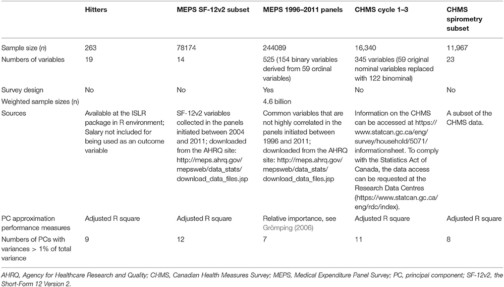
There were five data sets of various sizes used to understand the performance of PC approximation in Table 1. The first one, Hitters, was a small data set with 20 variables from a R package and was also a textbook example to demonstrate variable selection for multiple regression (James et al., 2013). Except for the outcome variables, “Salary,” all other variables were used for PCA and approximation. The second one contained the information on physical and mental health, the SF-12v2 (Short-Form 12 version 2) questionnaire (Ware et al., 1996), used to interview subjects aged 18 years or over in the first years of the 2-year panels in the Medical Expenditure Panel Survey (MEPS) implemented between 2004 and 2011 (Center for Financing Access and Cost Trends, 2014). The subjects did not respond to the SF-12v2 questions were discarded.
The third data set contained the 426 non-redundant first-year variables collected from interviewees age 0–90 years in the MEPS initiated between 1996 and 2011 (Chao, 2015; Chao et al., 2017). These variables were selected from 1991 variables common to these panels. The redundant variables with Spearman's correlation more than 0.9 were removed (Hall and Smith, 1997). The missing values in the 426 variables were imputed and log transformed if skewness was reduced with log transformation. There were 60 ordinal variables transformed to 156 binary variables and this led to 522 variables in total for PCA (see Data Sheet 1 for detail).
The fourth one included non-redundant variables from the Canadian Health Measures Survey (CHMS), we first selected variables with a correlation-based method that was designed in part to remove redundant variables and increasing computational feasibility (Hall and Smith, 1997; Saeys et al., 2007; Chao et al., 2018). The data redundancy might be created for the ease of survey implementation or data processing or concerns in measurement failures. For example, the food frequencies were reported in numbers per year and derived from daily, weekly, and annually intake. The spirometry could be tried for multiple times and the measurements of eight trials were documented in different variables (Chao et al., 2018). The details in the CHMS variables could be found in Data Sheet 2.
The last one was the spirometry subset of the CHMS data. There were 23 variables documenting the first trial of lung function tests and 11,967 subjects with complete measurement (see Data Sheet 2 for details). Among all lung function variables, forced expiratory volume in 1 s (FEV1), forced vital capacity (FVC) and the ratio of FEV1 and FVC (FEV1/FVC) were used as diagnostic criteria and important indicators of lung functions (Pierce, 2005; Quanjer et al., 2012). FVC measured the air volume that could be blown out with force and FEV1 was regarded as an indicator of chronic obstructive pulmonary disease across age groups (Fletcher and Peto, 1977). FEV1/FVC served as an indicator to distinguish restrictive or obstructive lung defect (Pierce, 2005).
Principal Component Analysis and Interpretation
The variables in the data sets were first centered and scaled before PCA. The first of the two interpretation methods was to show how information from all variables was aggregated to each PC. First, the input variables were sorted according to the descending order of the absolute values of loadings. The loadings were squared to estimate the proportions of variable variance contributed to each PC by input variables.
The other interpretation method was to conduct forward-stepwise regression (Hastie et al., 2009) to predict PCs with input variables. For each PC, we began with null model that did not contain any independent variables. By searching for the variable that improved the model performance the most in terms of Bayesian information criterion (BIC), we gradually increased the number of predictors in the selection process (Lumley and Lumley, 2004). We allowed all of the input variables to be used for approximation in each data set. Because of our interested in by how much R squared adding one more variables could increase, the incremental increase of R squared by adding one more variables in the forward selection was calculated. However, forward selection was not applicable to the third data set under complex survey design. Instead, we assessed the relative importance of independent variables that aim to show the breakdown of total R squared, one, to all independent variables in the model (Grömping, 2006). The sum of R squared of all independent variables regarding each PC was set to one.
The results of two approximation methods were illustrated with (1) line charts with the accumulated R squared for PCs and (2) mosaic plots (Theus and Urbanek, 2008) that demonstrated the distribution or redistribution of total variances by PCs and input variables. In the horizontal axes of the mosaic plots, the total variances of the data sets were projected to columns representing PCs. In each PC column of the mosaic plots, the variances contributed by variables to each PC was ordered by proportions of contributed variances (first approximation methods for all data sets) or incremental R squared in forward selection or relative importance of all input variables in terms of R squared. P < 0.05, two-tailed, were considered statistically significant. All analyses were conducted with R (v 3.22) (R Development Core Team, 2016) and RStudio (R Studio Team, 2016).
Performance of PC Approximation
We developed three criteria to assess the results of PC approximation. First, the efficiency of PC approximation by the first variables was assessed with R squared (Hastie et al., 2009) or relative importance measured in R squared (Grömping, 2006). Second, the efficacy of PC approximation was expressed by the differences in the areas under curves (AUCs) between the curves of accumulated squared loadings of input variables and those of the R squared of PC approximation curves. The accumulated squared loadings were ordered from large to small and summed sequentially. The curves represented the accumulated sums were plotted. On the other hand, the R squared of the PC variances explained by input variables that were selected based on forward-stepwise regression models were ordered from large to small. The curves represented the accumulated sums of R squared were also plotted. The differences in the AUCs were divided by the total area of the plots to obtain differences in the AUCs by proportions of total plotting areas. Last, the sparsity was represented by the numbers of input variables required to explain more than 80% of PC variances.
Results
Ordinary PCA was implemented with the data sets listed in Table 1. Total variances equaled the numbers of input variables or PCs. The input variables were summed together based on the loadings for each PC. The first few PCs had variances greater than the others. For example, the first PCs could explain 38.3%, 54.8%, 48.2%, 12.1%, and 50.3% of total variances in the five data sets, respectively. The relationships between the first two PCs in the first three data sets were shown in Figure 1. Scatter plots of the CHMS data were not allowed to be released for confidentiality reasons. The red and black coloring was based on the first variables selected in the process of approximating first PCs in forward-stepwise regression. These selected variables seemed to perform well in classifying observations into two major groups, especially for the Hitters data set.
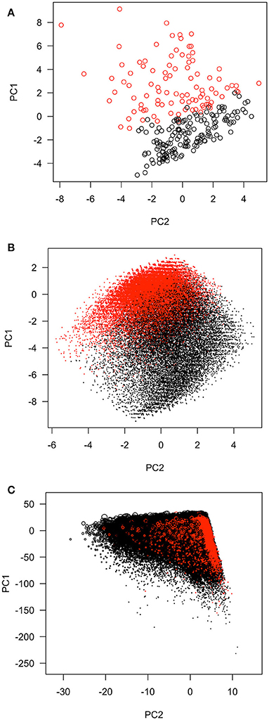
Figure 1. The distributions of first two principal components of the data sets. (A) The Hitters data set. Red: observations with CRBI (career runs batter in, the variable first selected in the stepwise regression to approximate the first principal component) >330; Black: observations with CRBI ≤ 330. (B) The MEPS SF-12 v2. subset. Red, observations with little or none of the time being limited in kind of work or other activities as result of physical health during past four weeks (variable name: adpwlm2, the variable first selected in the stepwise regression to approximate the first principal component); Black, some or most or all of the time being limited in kind of work or other activities. (C) The MEPS 1996–2011 panels. MEPS, Medical Expenditure Panel Survey; PC, principal component; SF-12v2, the Short-Form 12 Version 2. Red, subjects with the amounts of workers' compensation larger than zero; Black, subjects without any workers' compensation.
Variances Contributed According to Squared Loadings in Each PC
The first charts of Figures 2–6 showed the accumulative proportions of PC variances by adding the input variables according to the values of loadings in each PC. The curves of the squared loadings of the first PCs tended to be the lowest ones. This suggested that the creation of first PCs required contributions from the majorities of the input variables. Simply summing the products of the leading input variables and their loadings would not result in high-percentage approximation of first PCs. However, for the other PCs, the curves of squared loadings could reach the top, optimal approximation of PCs, sooner than the first four or five PCs.
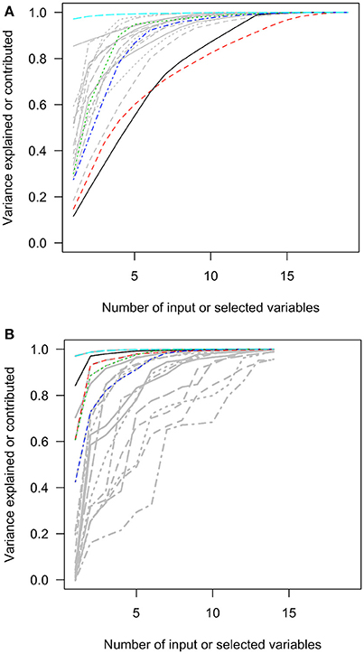
Figure 2. The squared loadings in each PC and the R squared of PC approximation in the Hitters data set. (A) The squared loadings of all variables in PCs. (B) The adjusted R squared of the variables that were used to approximate PCs. PC, principal component; black, first PC; red, second PC; green, third PC; blue, fourth PC; light blue, fifth PC.
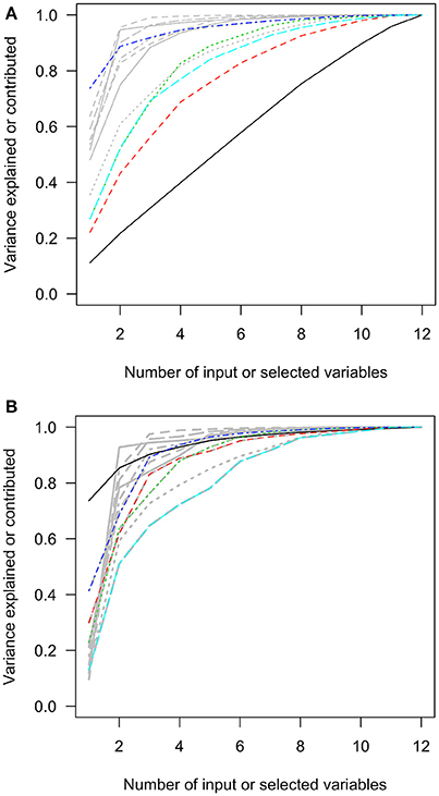
Figure 3. The squared loadings in each PC and the R squared of PC approximation in the MEPS SF-12v2 subset data. (A) The squared loadings of all variables in PCs. (B) The adjusted R squared of the variables that were used to approximate PCs. MEPS, Medical Expenditure Panel Survey; PC, principal component; SF-12v2, the Short-Form 12 Version 2. Black, first PC; red, second PC; green, third PC; blue, fourth PC; light blue, fifth PC.
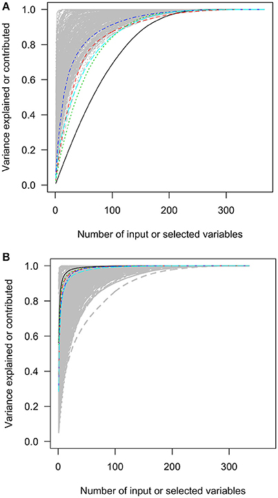
Figure 4. The squared loadings in each PC and the R squared of PC approximation in the Medical Expenditure Panel 1996–2011 panel data. (A) The squared loadings of all variables in PCs. (B) The adjusted R squared of the variables that were used to approximate PCs. PC, principal component. Black, first PC; red, second PC, green; third PC; blue, fourth PC; light blue, fifth PC.
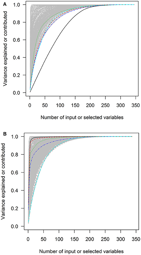
Figure 5. The squared loadings in each PC and the R squared of PC approximation in the Canadian Health Measures Survey cycle 1–3 data. (A) The squared loadings of all variables in PCs. (B) The adjusted R squared of the variables that were used to approximate PCs. PC, principal component. Black, first PC; red, second PC; green, third PC; blue, fourth PC; light blue, fifth PC.
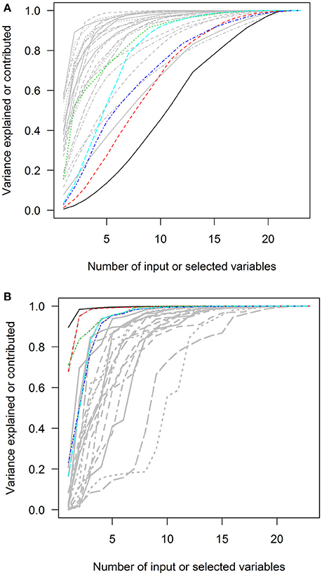
Figure 6. The squared loadings in each PC and the R squared of PC approximation in the Canadian Health Measures Survey spirometry subset. (A) The squared loadings of all variables in PCs. (B) The adjusted R squared of the variables that were used to approximate PCs. PC, principal component. Black, first PC; red, second PC; green, third PC; blue, fourth PC; light blue, fifth PC.
In contrast, the variables selected with forward-stepwise regression could result in better approximation of PCs in the second charts of Figures 2–6. The variables selected from the forward selection could reach the top with fewer numbers of variables than the approximation by loading orders, especially for the first few PCs.
Performance of PC Approximation
The R squared of the first variables to approximate PC1 and PC2 were listed in Table 2. According to the criteria we developed to compare the performance of PC approximation, the efficacy of forward-stepwise regression was better because the starting points of the first five PC approximation curve of forward selection were much higher than the approximation curves based on loadings in Figures 2–6. For the efficacy of PC approximation regarding PC1 and PC2, the proportions of the differences in the AUCs between two methods were listed in Table 2. The starting values of R squared were especially higher in data sets with fewer variables, Hitters and MEPS SF-12v2 subset, reaching 0.843 and 0.737 for the first PC, respectively. The p-values of the input variables were < 0.05.
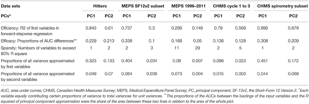
Table 2. Performance of principal component approximation with forward-stepwise regression in the data sets.
The higher positions of the approximation curves of forward selection indicated better efficacy in PC approximation. The improvement in efficacy was larger for PC1 in the five data sets. The differences in the AUCs between these two approximation methods were 0.229, 0.338, 0.168, 0.136, and 0.308 of total plotting areas for PC1 in the data sets (Table 2).
To reach at least 80% of R squared in PCs, the approximation using PCA loading required more variables than that using forward-stepwise selection. In Table 2, the numbers required to exceed 80% R squared for the first PCs were 1, 2, 11, 2, and 1 for the Hitters, MEPS SF-12v2 subset, MEPS 1996–2011 panels, CHMS cycle 1–3, and CHMS spirometry subset data sets, respectively. More variables were needed for the second PCs in the data sets.
The concept of sparsity in PC approximation could be illustrated in Figures 7–11. The variances of all variables were distributed to all PCs after PCA in the first charts. The columns were separated by solid gray lines and represented PCs. The widths of vertical columns were proportional to the PC variances. The first to the last PCs were sorted from left to right according to the PC variances. In each column, there were cells representing the input variables. The variances contributed by or explained by input variables were proportional to the cell volumes. The leading cell volumes were labeled with the percentages of total variances explained. The leading input variables for the PCs were rarely the same. For limited space, the variable names were not labeled. The gray area was where the cell sizes were smaller than the line widths. The eight leading variables in each column were colored.
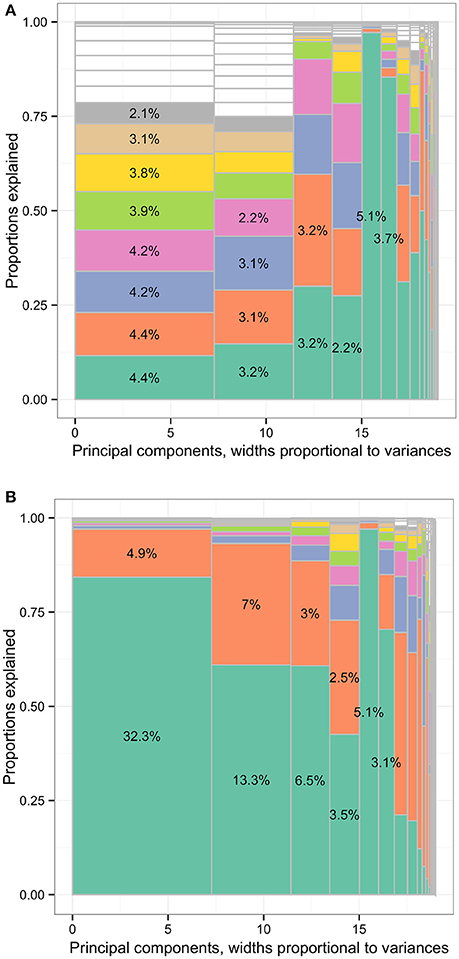
Figure 7. The distribution of total variances by principal components and input variables or approximation variables in the Hitters data set. Principal components, widths proportional to variances. (A) The distribution of total variances by principal components and input variables. Principal components, widths proportional to variances. (B) The distribution of total variances by principal components and approximation variables. The percentages in the cells representing the percentages of variances relative to total variance (whole area) based on the loadings of principal component analysis (first charts) or R squared. Each column represented the principal components (PCs) and had widths the same as the PC variance. In each column, the cells were of unequal sizes representing the variances explained by the input variables. For each PC specified in each column, the PC was explained by input variables. The cells in each column represented the input variables. The cell sizes were proportional to how much the PCs were explained by input variables. The cells were ordered by the variances explained by input variables or cell sizes. The variable names were not specified in the graph for limited spaces. The eight leading cells in each PC column were colored as a visual aid to highlight the numbers of input variables used to interpret the PCs. The cells of leading sizes were labeled with the proportions of total variances. The gray area represented the cells of small sizes and the cells were in gray color because the sizes of the white cells were smaller than the line widths of gray color.
In the first charts of Figures 7–11, how the variable variances were added according to PCA loadings was plotted. Each input variable projected some of its variances to PCs. The cells representing variables were ordered by the absolute values of loadings. In each PC column, the cell volumes representing variances projected by input variables according to loadings were relatively small.
However, in the second charts of Figures 7–11, each cell represented PC variances explained by input variables according to forward-stepwise regression. There were disproportionately large shares of total variances being explained by the first variables in the first PCs. The leading input variable approximating PC1 could explain as much as 32.3%, 40.4%, 7.9%, 9.6%, and 45.1% of total variances for the Hitters, MEPS SF-12v2 subset, MEPS 1996–2011 panels, CHMS cycle 1–3, and CHMS spirometry subset data sets, respectively, also listed in Table 2. Large cells representing large proportions of total variances explained tended to locate in the first two PC columns. There were more columns in the second charts where the input variables could approximate more than half of the PC variances.
Interpretation of PCs Through Approximation
In Figure 7B, the leading variables approximating PC1 were CRBI (number of runs batted in during his career) and runs (number of runs in 1986), associated with 32.3% and 4.9% of total variance in the data set, respectively. More than 97% of the PC1 variance was explained by these two variables. The leading variables approximating PC2 were AtBat (number of times at bat in 1986) and CAtBt (number of times at bat during his career), associated with 13.3% and 7.0% of total variance. More than 93% of PC2 variance was explained by these two variables. The leading variables approximating PC3 were League (player's league at the end of 1986) and Assists (number of assists in 1986), explaining 6.5% and 3.0% of total variance. More than 88% of PC3 variance was explained by these two variables.
In Figure 8B, the leading variables approximating PC1 were work limit because of physical problems (variable name: adpwlm2 in Data Sheet 1) and accomplishing less because of mental problems (admals2), associated with 40.4% and 6.4% of total variance in the data set, respectively. More than 85% of PC1 variance was explained by these two variables. The leading variable approximating PC2 were feeling calm or peaceful (adcape2), health limiting moderate activities (addaya2), and feeling downhearted or depressed (addown2), associated with 3.4%, 3.6%, and 2.4% of total variance, respectively. More than 83% of PC2 variance was explained by these three variables.
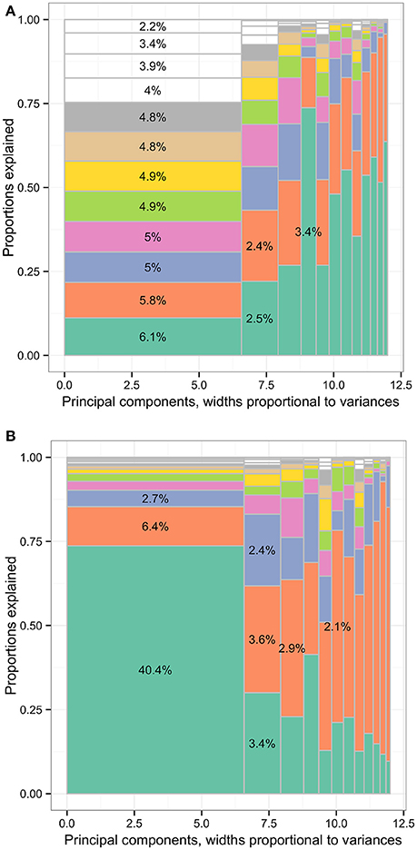
Figure 8. The distribution of total variances by principal components and input variables or approximation variables in the MEPS SF-12v2 dataset. Principal components, widths proportional to variances. (A) The distribution of total variances by principal components and input variables. Principal components, widths proportional to variances. (B) The distribution of total variances by principal components and approximation variables. MEPS, Medical Expenditure Panel Survey; SF-12v2, the Short-Form 12 Version 2. The percentages in the cells representing the percentages of variances relative to total variance (whole area) based on the loadings of principal component analysis (first charts) or R squared. Each column represented the principal components (PCs) and had widths the same as the PC variance. In each column, the cells were of unequal sizes representing the variances explained by the input variables. For each PC specified in each column, the PC was explained by input variables. The cells in each column represented the input variables. The cell sizes were proportional to how much the PCs were explained by input variables. The cells were ordered by the variances explained by input variables or cell sizes. The variable names were not specified in the graph for limited spaces. The eight leading cells in each PC column were colored as a visual aid to highlight the numbers of input variables used to interpret the PCs. The cells of leading sizes were labeled with the proportions of total variances. The gray area represented the cells of small sizes and the cells were in gray color because the sizes of the white cells were smaller than the line widths of gray color.
In Figure 9B, the leading variables approximating PC1 were workers' compensation amounts (wcmppy1x, see Data Sheet 2 for variable details), poverty categories (povcaty1), marital status (marryy1x.5 and marryy1x.3), activity limitations (actlim1.2), and self-perceived health status (rthlth1), associated with 12.5%, 12.1%, 4.9%, 2.1%, 1.4%, and 1.1% of total variance of the data set, respectively. The percentages were relatively large compared to the maximal percentages single input variables could contribute to PC1 in Figure 9A, 0.2%.
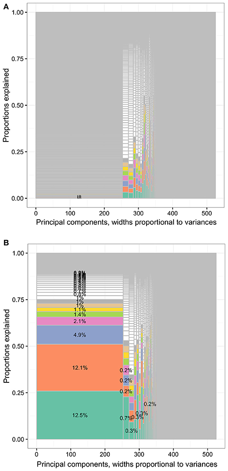
Figure 9. The distribution of total variances by principal components and input variables or approximation variables in the MEPS 1996–2011 panels. Principal components, widths proportional to variances. (A) The distribution of total variances by principal components and input variables. Principal components, widths proportional to variances. (B) The distribution of total variances by principal components and approximation variables. MEPS, Medical Expenditure Panel Survey. The percentages in the cells representing the percentages of variances relative to total variance (whole area) based on the loadings of principal component analysis (first charts) or R squared. Each column represented the principal components (PCs) and had widths the same as the PC variance. In each column, the cells were of unequal sizes representing the variances explained by the input variables. For each PC specified in each column, the PC was explained by input variables. The cells in each column represented the input variables. The cell sizes were proportional to how much the PCs were explained by input variables. The cells were ordered by the variances explained by input variables or cell sizes. The variable names were not specified in the graph for limited spaces. The eight leading cells in each PC column were colored as a visual aid to highlight the numbers of input variables used to interpret the PCs. The cells of leading sizes were labeled with the proportions of total variances. The gray area represented the cells of small sizes and the cells were in gray color because the sizes of the white cells were smaller than the line widths of gray color.
In Figure 10B, the leading input variables to approximate PC1 of the CHMS cycle 1–3 data set were hours in physical activities at school per week, blood pressure categories, self-reported weight, and alcohol drinking that accumulatively explained 79.0%, 91.2%, 94.1%, and 95.2% of PC1 variance. The leading variables regarding PC2 were forced expiratory flow at 75% (FEF75%) of forced vital capacity (FVC), largest forced expiratory volume (FEV) at 3rd second from acceptable efforts, predicted ratios of forced expiratory volume at 1st second and forced vital capacity (FEV1/FVC), and total steps at second days of 1-week monitoring that accumulatively explained 56.9%, 64.7%, 75.0%, and 79.3% of PC2 variance. The leading variables regarding PC3 were total light physical activity in minutes, time wearing activity monitors and total steps that accumulatively explained 37.0%, 50.6%, and 59.6% of PC3 variance.
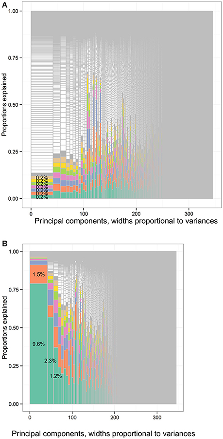
Figure 10. The distribution of total variances by principal components and input variables or approximation variables in the Canadian Health Measures Survey cycle 1–3 data set. Principal components, widths proportional to variances. (A) The distribution of variances of the full data set of the CHMS cycle 1 to 3 according to the PCA loadings. There were 345 columns separated by solid vertical gray lines. Principal components, widths proportional to variances. (B) The distribution of variances of the full data set of the CHMS cycle 1–3 according to the forward regression. There were 345 columns separated by solid vertical gray lines. CHMS, Canadian Health Measures Survey; PCA, principal component analysis. Each column represented the principal components (PCs) and had widths the same as the PC variance. In each column, the cells were of unequal sizes representing the variances contributed by the input variables. The cells in each column represented the input variables. The cell sizes were proportional to the variances that the input variables contributed to PCs. The cells were ordered by the variances contributed by input variables or cell sizes. The variable names were not specified in the graph for limited spaces. The eight leading cells in each PC column were colored as a visual aid to highlight the numbers of input variables used to interpret the PCs. The cells of leading sizes were labeled with the proportions of total variances. The gray area represented the cells of small sizes and the cells were in gray color because the sizes of the white cells were smaller than the line widths of gray color. The cells of leading sizes were labeled with the proportions of total variances. The gray area represented the cells of small sizes.
In Figure 11B, the leading variables to approximate the PC1 of the spirometry subset were FEV0.5/FVC (%) and FEV1/FVC (%), accumulatively explaining 89.6% and 98.4% of PC1 variance. The leading variables to approximate the PC2 were forced expiratory volume in 0.75 s (L) and FEV0.5/FVC (%), accumulatively explaining 67.9% and 95.1% of PC2 variance. The leading variables to approximate PC3 were back-extrapolated volume (fraction of FVC) and expiratory time in seconds, accumulatively explaining 71.2% and 83.7% of PC3 variance.
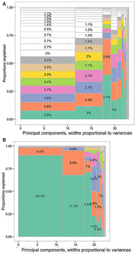
Figure 11. The distribution of total variances by principal components and input variables or approximation variables in the Canadian Health Measures Survey spirometry subset data set. Principal components, widths proportional to variances. (A) The distribution of variances of the spirometry subset according to the PCA loadings. There were 23 columns separated by solid vertical gray lines. Principal components, widths proportional to variances. (B) The distribution of variances of spirometry subset of the CHMS cycle 1 to 3 according to the forward regression. There were 23 columns separated by solid vertical gray lines. CHMS, Canadian Health Measures Survey; PCA, principal component analysis. Each column represented the principal components (PCs) and had widths the same as the PC variance. In each column, the cells were of unequal sizes representing the variances explained by the input variables. For each PC specified in each column, the PC was explained by input variables. The cells in each column represented the input variables. The cell sizes were proportional to how much the PCs were explained by input variables. The cells were ordered by the variances explained by input variables or cell sizes. The variable names were not specified in the graph for limited spaces. The eight leading cells in each PC column were colored as a visual aid to highlight the numbers of input variables used to interpret the PCs. The cells of leading sizes were labeled with the proportions of total variances. The gray area represented the cells of small sizes and the cells were in gray color because the sizes of the white cells were smaller than the line widths of gray color.
Identification of Unique Sources of Variances
Besides PC1 and PC2, there were other PCs were approximated with relatively few numbers of input variables. For the Hitters data set, 97.0% of the PC5 variance was explained by one variable, Division. This variable was very specific to PC5 and was not the first five leading variable to approximate other PCs. There were 88.6% and 85.0% of the PC3 and PC6 variances explained by only two input variables. For the MEPS SF12 subset, 81.0%, 92.8%, and 85.2% of the PC10, PC11, and PC12 variances were explained by two input variables. For the full MEPS data set, more than 80% of the variances of 11, 31, 53, and 58 PCs could be approximated with two, three, four, and five input variables, while it took five variables to explain 80.6% of PC1 variance. For the CHMS cycle 1–3 data set, more than 80% of the variances of 3, 6, and 11 PCs could be approximated with two, three, and four input variables, respectively. For the CHMS spirometry subset, more than 80% of the variances of PC1, PC2, and PC3 could be explained by two input variables. In addition, more than 80% of PC5, PC10, and PC16 could be explained by three input variables.
Discussion
The results show that PCs can be approximated with differing levels of efficiency (proportions of variance explained by first variables), efficacy (differences in the AUCs of total variances), and sparsity (numbers of variables to explain more than 80% of PC variances). This shows that PCs can be effectively approximated with relatively few numbers of variables, especially for the first PCs of the data sets. The leading input variables to approximate PCs based on forward-stepwise regression can explain large shares of variances in the first and second PCs, and thus total variances.
This finding has several practical implications. First, PC approximation helps to interpret and understand the values of PCs. PCA is often used for dimension reduction or data compression. One drawback is the lack interpretability of the PCs because PCs are generated with information from all input variables (Hastie et al., 2009). Although the loadings of PCs can help researchers understand the relative importance of input variables in PCs, this method of interpretation remain unsatisfactory in large data sets (Hastie et al., 2009; Chao et al., 2017). The results show that PCs can be explained by fewer numbers of variables, rather than interpreting PCs as the summation of all variables. Our illustration shows that the first and second PCs can be largely approximated with relatively fewer variables, especially for the 19-variable data set, Hitters.
Second, the variables approximating first few PCs are important clues for further data compression or information retrieval. Currently, several of the first PCs that explain large portions of total variances are often used to approximate whole data sets (Hastie et al., 2009). For example, large image data can sometimes be mostly recovered with few PCs. The PCs of independent variables in research databases can be used for regression analysis or principal component regression (Hastie et al., 2009). Our methods show that by approximating the first few PCs, it is possible to identify variables that have dominant roles in explaining total variances in data sets. By approximating the first few PCs with input variables, we can use the leading variables to understand the major sources of information in a data set or use fewer variables to recover information. This is important since PCA is often used for exploratory analysis and unsupervised learning (Hastie et al., 2009). Researchers use PCA as a means to obtain initial impression of the data and proceed with other methods, especially supervised learning methods. The approximation method can help researchers to begin with one or two leading variables of relevance. Based on our study, prioritizing input variables through identifying major sources of variances is proven helpful to target variables for data cleaning and inspection.
For the spirometry subset, the leading variables identified via PC approximation using forward regression are not exactly the same as the respiratory function measures most heavily used by respiratory care specialists. For the diagnosis of lung disease, FVC, FEV1, and FEV1/FVC are important indicators to distinguish obstructive and restrictive lung diseases (Pierce, 2005). However, we find that FEV0.5/FVC, FEV0.75, and FEV1/FVC can explain more than 45.1%, 17.2%, and 5.5% of total variance in the first trial of spirometry in general Canadians. This may suggest that a large portion of the information gathered in a spirometry test is not used. We plan to investigate the usefulness of these highly relevant variables identified with PC approximation. Our preliminary research finding is that lung function represents a unique trajectory across individuals aged 3–79 years and FEV0.5/FVC remains important to explain the lung function trajectory throughout the age spectrum (Chao et al., 2018).
Third, there are several unique sources of variances identified in the test data sets. There are variables that specifically resemble certain PCs. For example, “Division” in the Hitters data set predicts the fifth PC very well and has little correlation with other variables. There are many other combinations of input variables resembling other PCs. For the orthogonality properties of PCs, these variables provide information less correlated with other PCs and may be treated as sources of unique information for further investigation.
Lastly, PC approximation can be especially meaningful while searching for the variables that may be neglected in empirical evidence or should be prioritized for investigation. For example, we may think of the dimensions of the SF-12v2 questionnaire equally important because they are representative of the response categories of mental and physical health. However, the limitations in work or related activities are the leading variable to explain total variances and document the variations across individuals in similar population as those in the MEPS SF-12v2 subset. This may be because this population has more individuals of working age. The limitations in work become the most important contributor to between-individual variations. For the MEPS data, it is surprising to find the amount of workers' compensation is the leading variables to explain total between-individual variances. However, the other leading variables are those familiar to researchers, including poverty category, marital status, and limitations in work, household, or school.
Strengths and Limitations
The results from the data sets of different dimensions seem to agree upon the feasibility of PC approximation with stepwise regression to improve interpretability of PCs, especially the first two PCs. However, there are still some limitations for this proposed approach. First, forward-stepwise regression was not feasible with data under survey design. The R-squared for the third data set is derived from the relative importance assessment and this may not be totally compatible with conventional R-squared. Second, there are data sets that may not be ideal for PCA and thus PC approximation. For example, if there are more numbers of variables than observations, ordinary, or linear PCA is not appropriate. If there are too many unlabeled or undefined variables, the leading variables that explain large proportions of PC variances may not be readily understandable. In these cases, PC approximation may not be ideal.
Future Work
We also identify the opportunities to develop new data methods. First, there are other dimension reduction methods to be tried. PCA is one of the linear or non-linear methods to generate eigenvectors (Hastie et al., 2009). We will extend the concept of approximation to eigenvectors generated with other methods, such as isometric feature mapping and local linear embedding (Hastie et al., 2009). Second, the evaluation criteria of PC approximation, efficacy, efficiency, and sparsity, are up for discussion and still under development.
Conclusion
The PCs can be approximated with input variables according to the loadings or the results from stepwise regression. The approximation with stepwise regression can be used to interpret PCs, identify major sources of variances, select unique sources of information in data sets, and search for variables that may be neglected and awaiting further examination. The performance of PC approximation with stepwise regression differs in various data sets. For data sets with fewer numbers of variables, approximating PC can be very effective with few input variables. In general, the approximation of first two PCs seems to be the most effective and useful for researchers and worth further investigation for small or large data sets such as the MEPS data.
Data Availability
The Hitters data set can be assessed within R package, ISLR. The Medical Expenditure Panel Survey data can be freely downloaded (https://meps.ahrq.gov/data_stats/download_data_files.jsp). It is against the Statistics Act of Canada to release the Canadian Health Measures Survey data. The data access can be obtained through the Research Data Centres program (https://www.statcan.gc.ca/eng/rdc/index).
Ethics Statement
This secondary data analysis study was approved by the ethics committee of the Centre hospitalier de l'Université de Montréal (2016-6095, CE 15.115—CA). There was no identifiable information. The written and informed consent from the participants was not required according to the Ethics Committee that approved the study.
Author Contributions
Y-SC conceptualized the research project, restructured the data, conducted the statistical analyses, and drafted the manuscripts. H-CW, C-JW, and W-CC reviewed the manuscript and provided constructive comments.
Funding
Y-SC was financed by the Fonds de recherche du Québec—Santé (FRQS) fellowship. The granting agencies had no role in this study.
Conflict of Interest Statement
The authors declare that the research was conducted in the absence of any commercial or financial relationships that could be construed as a potential conflict of interest.
Supplementary Material
The Supplementary Material for this article can be found online at: https://www.frontiersin.org/articles/10.3389/fdigh.2018.00011/full#supplementary-material
Data Sheet 1. The characteristics of the MEPS variables.
Data Sheet 2. The characteristics of the CHMS variables.
References
Allen, G. I., and Maletic-Savatic, M. (2011). Sparse non-negative generalized PCA with applications to metabolomics. Bioinformatics 27, 3029–3035. doi: 10.1093/bioinformatics/btr522
Barshan, E., Ghodsi, A., Azimifar, Z., and Jahromi, M. Z. (2011). Supervised principal component analysis: visualization, classification and regression on subspaces and submanifolds. Pattern Recogn. 44, 1357–1371. doi: 10.1016/j.patcog.2010.12.015
Bodor, A., Csabai, I., Mahoney, M. W., and Solymosi, N. (2012). rCUR: an R package for CUR matrix decomposition. BMC Bioinformatics 13:103. doi: 10.1186/1471-2105-13-103
Center for Financing Access and Cost Trends (2014). MEPS HC-156: Panel 16 Longitudinal Data File, Agency for Healthcare Research and Quality, Editor. Rockville, MD: Agency for Healthcare Research and Quality.
Chao, Y.-S. (2015). “Life stages and trajectories in the medical expenditure survey 1996 to 2011,” in 13e Édition des Journées de Recherche RQRV (Montreal, QC: Réseau Québécois de Recherche sur le Vieillissement).
Chao, Y.-S., Wu, H. C., Wu, C.-J., and Chen, W. C. (2018). Stages of biological development across age: an analysis of canadian health measure survey 2007–2011. Front. Public Health 5:355. doi: 10.3389/fpubh.2017.00355
Chao, Y.-S., Wu, H.-T., and Wu, J.-C. (2017). Feasibility of classifying life stages and searching for the determinants: results from the medical expenditure panel survey 1996–2011. Front. Public Health 5:247. doi: 10.3389/fpubh.2017.00247
Fletcher, C., and Peto, R. (1977). The natural history of chronic airflow obstruction. Br. Med. J. 1, 1645–1648.
Gandomi, A., and Haider, M. (2015). Beyond the hype: big data concepts, methods, and analytics. Int. J. Inform. Manag. 35, 137–144. doi: 10.1016/j.ijinfomgt.2014.10.007
Goreinov, S. A., Tyrtyshnikov, E. E., and Zamarashkin, N. L. (1997). A theory of pseudoskeleton approximations. Linear Algebra Appl. 261, 1–21. doi: 10.1016/S0024-3795(96)00301-1
Grömping, U. (2006). Relative importance for linear regression in R: the package relaimpo. J. Stat. Softw. 17, 1–27. doi: 10.18637/jss.v017.i01
Hall, M. A., and Smith, L. A. (eds.). (1997). “Feature subset selection: a correlation based filter approach,” in International Conference on Neural Information Processing and Intelligent Information Systems (Berlin: Springer).
Hastie, T., Tibshirani, R., and Friedman, J. (2009). The Elements of Statistical Learning: Data Mining, Inference, and Prediction, 2nd Edn. New York, NY: Springer.
Hulten, G., Spencer, L., and Domingos, P. (2001). “Mining time-changing data streams,” in Proceedings of the Seventh ACM SIGKDD International Conference on Knowledge Discovery and Data Mining (San Francisco, CA: ACM).
James, G., Witten, D., Hastie, T., and Tibshirani, R. (2013). An Introduction to Statistical Learning: With Applications in R. New York, NY: Springer.
Johnstone, I. M., and Lu, A. Y. (2009). On consistency and sparsity for principal components analysis in high dimensions. J. Am. Stat. Assoc. 104, 682–693. doi: 10.1198/jasa.2009.0121
Lumley, T. (2004). Analysis of complex survey samples. J. Stat. Softw. 9:19. doi: 10.18637/jss.v009.i08
Lumley, T. (ed.). (2011). Complex Surveys: A Guide to Analysis Using R, Vol. 565. Hoboken: John Wiley & Sons.
Lumley, T., and Lumley, M. T. (2004). The Leaps Package. Vienna: R Project for Statistical Computing. Available online at: https://cran.r-project.org/web/packages/leaps/leaps.pdf
Mahoney, M. W., and Drineas, P. (2009). CUR matrix decompositions for improved data analysis. Proc. Natl. Acad. Sci. U.S.A. 106, 697–702. doi: 10.1073/pnas.0803205106
Quanjer, P. H., Stanojevic, S., Cole, T. J., Baur, X., Hall, G. L., Culver, B. H., et al. (2012). Multi-ethnic reference values for spirometry for the 3-95-yr age range: the global lung function 2012 equations. Eur. Respir. J. 40, 1324–1343. doi: 10.1183/09031936.00080312
R Development Core Team (2016). R: A Language and Environment for Statistical Computing. Vienna: R Foundation for Statistical Computing.
Saeys, Y., Inza, I., and Larranaga, P. (2007). A review of feature selection techniques in bioinformatics. Bioinformatics 23, 2507–2517. doi: 10.1093/bioinformatics/btm344
Theus, M., and Urbanek, S. (2008). Interactive Graphics for Data Analysis: Principles and Examples. Boca Raton, FL: CRC Press.
Keywords: principal component analysis (PCA), principal component approximation, principal components (PCs), stepwise regression, loadings, Medical Expenditure Panel Survey (MEPS), Canadian Health Measures Survey (CHMS)
Citation: Chao Y-S, Wu H-C, Wu C-J and Chen W-C (2018) Principal Component Approximation and Interpretation in Health Survey and Biobank Data. Front. Digit. Humanit. 5:11. doi: 10.3389/fdigh.2018.00011
Received: 13 October 2017; Accepted: 09 May 2018;
Published: 26 June 2018.
Edited by:
Enrico Capobianco, University of Miami, United StatesReviewed by:
Satya S. Sahoo, Case Western Reserve University, United StatesLaetitia Jourdan, Lille University of Science and Technology, France
Copyright © 2018 Chao, Wu, Wu and Chen. This is an open-access article distributed under the terms of the Creative Commons Attribution License (CC BY). The use, distribution or reproduction in other forums is permitted, provided the original author(s) and the copyright owner are credited and that the original publication in this journal is cited, in accordance with accepted academic practice. No use, distribution or reproduction is permitted which does not comply with these terms.
*Correspondence: Wei-Chih Chen, d2lqaS5jaGVuQGdtYWlsLmNvbQ==
 Yi-Sheng Chao
 Hsing-Chien Wu
 Chao-Jung Wu
 Wei-Chih Chen