Active transfer learning for audiogram estimation

Computational audiology (CA) has grown over the last few years with the improvement of computing power and the growth of machine learning (ML) models. There are today several audiogram databases which have been used to improve the accuracy of CA models as well as reduce testing time and diagnostic complexity. However, these CA models have mainly been trained on single populations. This study integrated contextual and prior knowledge from audiogram databases of multiple populations as informative priors to estimate audiograms more precisely using two mechanisms: (1) a mapping function drawn from feature-based homogeneous Transfer Learning (TL) also known as Domain Adaptation (DA) and (2) Active Learning (Uncertainty Sampling) using a stream-based query mechanism. Simulations of the Active Transfer Learning (ATL) model were tested against a traditional adaptive staircase method akin to the Hughson-Westlake (HW) method for the left ear at frequencies $\omega =0.25,0.5,1,2,4,8$ kHz, resulting in accuracy and reliability improvements. ATL improved HW tests from a mean of 41.3 sound stimuli presentations and reliability of $\pm 9.02$ dB down to $25.3\pm 1.04$ dB. Integrating multiple databases also resulted in classifying the audiograms into 18 phenotypes, which means that with increasing data-driven CA, higher precision is achievable, and a possible re-conceptualisation of the notion of phenotype classifications might be required. The study contributes to CA in identifying an ATL mechanism to leverage existing audiogram databases and CA models across different population groups. Further studies can be done for other psychophysical phenomena using ATL.

1 Introduction

The World Health Organisation (WHO) estimates that more than 5% of the world’s population, approximately 430 million people, currently have a degree of hearing loss and require rehabilitation (1). The WHO further estimates that by 2,050, 2.5 billion people will have a degree of hearing loss with 700 million requiring rehabilitation. While the challenge of hearing loss is more common in low- to middle-income populations, the traditional assessment of hearing is not easily accessible to these populations because it is time-consuming and expensive.

Computational audiology (CA) has been shown to make hearing assessment more accessible (2) by for example, reducing diagnostic time from hours to a few minutes with significantly fewer stimuli presentations (3, 4), assessing both ears simultaneously (5), making distinctions at finer frequencies and intensity levels (6, 7) or even conducting assessment on a mobile phone without the aid of an audiology expert (5, 8, 9).

Nonetheless, CA has been slow to gain clinical acceptance (2) despite the cost, access and time limitations with traditional pure-tone audiometry (PTA). Other limitations of diagnostic tests include instances where some patients have received normal hearing results yet experience hearing loss (10), and errors especially in bone conduction tests (11).

One of the other advantages that CA brings is the ability to augment existing PTA diagnostic tests with other additional factors in audiogram estimation such as altitude, tympanogram data, otoscopic images, gender, age, medication history, noise exposure and many others, to result in precision audiology at low cost, reduced time and at a scale that will meet the demands of society with increasing hearing loss challenges (1). For example, Cox and De Vries (12) used age and gender to speed the accuracy of audiogram estimation, and Zhao et al. (13) used noise exposure at work to improve the accuracy. However, there are few or no CA studies that have investigated how the different additional factors influence hearing loss between different population groups, nor how to transfer Machine Learning (ML) models from one population group to another without losing computational model performance.

This study focused on contributing to CA by introducing Transfer Learning (TL) to identify informative priors using audiogram databases from different population groups, and to investigate the extent to which the informative priors from the different population groups can speed up audiogram estimation. TL is an area of ML that focuses on utilizing knowledge gained while solving an ML problem and applying the same knowledge to a different but related problem. Through TL, new systems can quickly adapt to new situations, tasks and environments by re-using pre-trained models (14). Like the similar notion of transfer of learning in the education discipline, TL addresses how learning in one context can be applied to learning in another context, often with better or faster solutions. The key benefits of TL are the maximization of limited ML and data resources, the re-use of the ML and data resources for different tasks, the beneficial adaptation of ML models to a new environment or different context, and the ability to navigate beyond the growing constraints around data because of privacy laws. This means that through TL, audiogram estimation can be performed for significantly less cost and in less time.

This study sought to answer two main research questions. First, how can Transfer Learning (TL) be used to identify informative priors from different population groups? Second, how can the informative priors speed up audiogram estimation?

2 Data preparation

Table 1 describes the pure-tone audiogram databases that were used in the study. The data is proprietary and obtainable from the Scalable Hearing Rehabilitation for Low- and Middle-Income Countries (SHRLMIC), Project reference: UNOPS/CFP-2020/001/ATSCALE. The project was funded by the United States Agency for International Development (USAID) in support of the Global Partnership for Assistive Technology (ATscale) and managed by the United Nations Office for Project Services (UNOPS).

Table 1

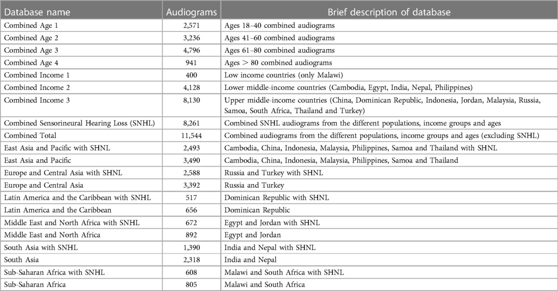
Table 1. Description of initial dataset of audiogram databases.

The project collected and aggregated audiogram data from various regions and countries, resulting in diverse and comprehensive audiogram databases. The data was also reorganized and classified collectively based on age and income groups, which allows for more nuanced analyses of global auditory health trends.

We decided to exclude the sensorineural hearing loss (SNHL) audiogram databases from the study due to their fundamental differences from normal conductive hearing loss audiograms. While the idea of transfer learning suggests that knowledge from one domain should be able to transfer to another, it was essential to consider the specific characteristics of each domain separately for now. SNHL and conductive hearing loss, while sharing knowledge and are related, exhibit distinct underlying physiological mechanisms and hearing profiles. By focusing on conductive hearing loss databases, we aimed to develop the model to the specific features and challenges of conductive hearing loss. We therefore considered that including SNHL audiograms in the model is an area for further research.

Duplicate audiograms and audiograms with missing values were removed. Outlier audiograms, that is, those with interaural gaps or $\ge 50$ dB in two or more thresholds were purposefully left in the data similar to Parthasarathy et al. (15) and Charih et al. (16) in order to better represent the prior information in its original context. We then explored the statistical features (Table 2) using the six frequency octaves: 250 Hz, 500 Hz, 1 kHz, 2 kHz, 4 kHz and 8 kHz.

Table 2

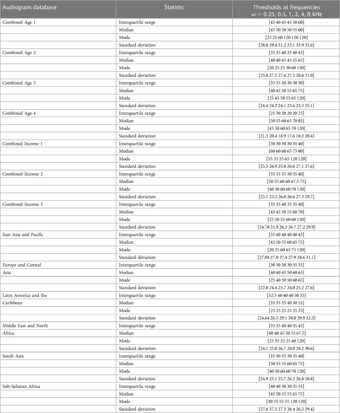
Table 2. Statistical characteristics of the audiogram databases.

3 Methods

We used an adaptive staircase method akin to the Hughson-Westlake (HW) method for its flexibility for use in computational modelling. The HW method uses reversals in intensity from increasing (or decreasing) intensities to identify the hearing thresholds. The more recent modified HW method is automated and remains popular among audiologists (17).

3.1 Transfer learning

There are three main tasks in TL. First, to identify “what” to transfer; second, to infer “how” to transfer; and third, to decide “when” to transfer based on whether TL was beneficial in the context.

3.1.1 What to transfer

The starting point was to recognize that all the original and reclassified audiogram databases shared several features, particularly in using between 6–8 frequency octave intervals for both ears. This means that all audiogram databases have a degree of homogeneity. There is however also a degree of heterogeneity in the databases usually from the different additional features such as age, gender, location, noisy environment at work and others. While these associated features are not mandatory, they are valuable in ML methods to uniquely determine patterns such as audiogram phenotypes. The first step was therefore to identify the extent of homogeneity, whether marginal probability $P(X_s\cap X_t)\ne 0$, and heterogeneity, whether $P(X_s\cap X_t)=0$ across the different audiogram databases.

Table 2 reveals descriptive heterogeneity between the audiogram databases. It is particularly noticeable that the median threshold value occurs from 40 dB HL upwards across all the frequencies in all the databases. This finding supports the choice of using 40 dB HL as recommended by Maltby (18) as a preferable starting intensity and one that is not uncomfortable for all types of patients.

Despite the descriptive heterogeneity, it was necessary to use an inferential method to specifically determine the extent of homogeneity or heterogeneity. We opted for a Gaussian Mixture Model (GMM) to infer the phenotypes within each of the databases because GMMs allow for soft clustering, that is, a data point can belong to more than one cluster in degrees (19). This is different from hard clustering where a data point belongs to strictly one cluster. GMMs are therefore ideal for modeling audiogram phenotype categories. Previous work by Cox and De Vries (12) used a GMM to introduce an informative prior as a prior distribution $p(t|a,g)$ in audiogram assessment conditioned on age $a\in \mathbb{N}$ and gender $g\in \{female|male\}$.

GMMs lean more towards being probabilistic distributions rather than being models because they are a combination of different Gaussian distributions (20). GMMs model discrete latent variables as a linear combination of Gaussians (20) in the form:vv

$p\text{( x) }=\sum _{k=1}^K{\pi }_k\mathcal{N}(x|{\mu }_k,{\mathrm{\Sigma }}_k)(1)$

where the Gaussian density $\mathcal{N}(x|{\mu }_k,{\mathrm{\Sigma }}_k)$ is a component of the mixture and has its own mean ${\mu }_k$ and covariance ${\mathrm{\Sigma }}_k$. ${\pi }_k$ is the mixing coefficient that represents the degree to which a data point fits within different clusters and is a valid probability such that $\sum _{k=1}^K{\pi }_k=1\text{ and }0\le {\pi }_k\le 1$.

The GMM is therefore governed by the parameters $\pi ,\mu \text{ and }\mathrm{\Sigma }$. The setting of the parameters using maximum likelihood makes the solution analytically complex (20) and takes it out of the closed form. Thus, our goal becomes the minimization of the negative log-likelihood loss function, $L$ 2:

$L(\pi ,\mu ,\mathrm{\Sigma })=-\sum _{i=1}^n\log (\sum _{k=1}^K{\pi }_k\mathcal{N}(x_i|{\mu }_k,{\mathrm{\Sigma }}_k))+\lambda \sum _{k=1}^K\Vert {\mathrm{\Sigma }}_k{\Vert }^2(2)$

where $\lambda$ is a regularization parameter. We included a regularization value of 0.01 in the loss function to ensure that the covariance matrix remained positive semi-definite.

We therefore used the Expectation Maximization (EM) method because of its ability to estimate the parameters in an iterative and efficient way.

We used k-means clustering with the gap statistic (21) to identify the optimum number of $K$ phenotypes. Figures 1, 2 present example phenotypes using the number of clusters identified using the k-means clustering method, in these examples, both 7 clusters. The two figures visually reveal the heterogeneity. Table 3 presents the phenotypes using the number of clusters identified and the ${\pi }_k$ as the mixing coefficients of each cluster.

Figure 1

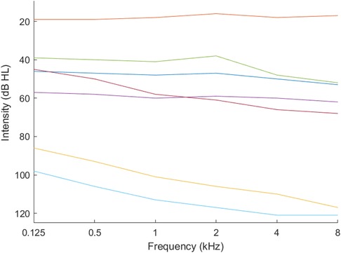
Figure 1. Phenotypes for ages 18–40 years.

Figure 2

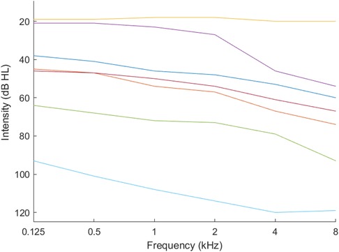
Figure 2. Phenotypes for combined income — upper middle income countries.

Table 3

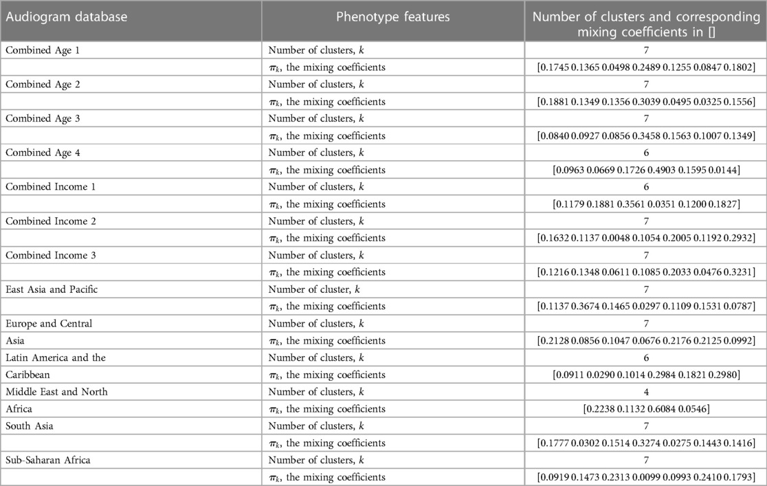
Table 3. Phenotypes of the audiogram databases and their characteristics.

Based on the number of clusters and the differences in the mixing coefficients (Table 3), and therefore the phenotypes, the audiogram databases were confirmed as heterogeneous, that is, the marginal probabilities $P(X_s\cap X_t)=0$. The covariance matrix sets were also heterogeneous, and the mean values in the component models were all different which also pointed to heterogeneity.

This finding limited the TL approach to feature-based options. The task was therefore to learn the mapping function $f_s(\cdot )\to f_t(\cdot )$ between the audiogram databases and the audiogram estimation required.

3.1.2 How to transfer

The results of the preceding step, “what to transfer”, are used to inform the “how to transfer”, whether through common features, instances, models or parameters.

We therefore turned to active learning, particularly stream-based active learning to identify informative features from the audiogram databases. In active learning, there is an intentionality about the profile being searched for in every query; that is, the next query is based on answers to the previous query (22). Based on the sets of answers, the model or classifier is improved continually.

We combined all the audiogram databases into one large dataset, and used the large dataset as the source data, $D_s$, from which to discover and extract good features to use in the audiogram estimation. Using the GMM, we discovered 18 phenotypes (Figure 3).

Figure 3

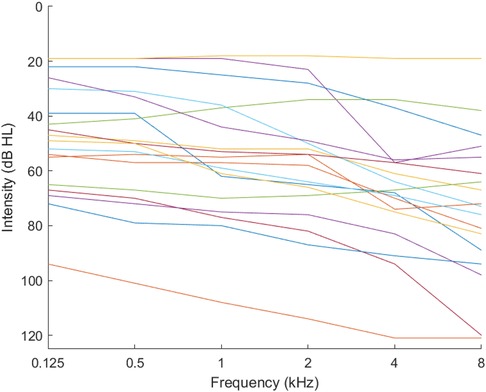
Figure 3. Phenotypes for combined audiograms.

We regarded the profile being searched for as that which is generated from the feature-based TL mapping function aimed at learning a pair of mapping functions $\{f_s(\cdot ),f_t(\cdot )\}$ to map data respectively from $D_s$ and $D_t$ to a common feature space, $D_c$, ($f_s(D_s)\mapsto D_c$ and $f_s(D_t)\mapsto D_c$) where the difference between $D_s$ and $D_t$ can be reduced. $D_c$ then serves as the input to the ML algorithm. We used feature augmentation (14, 23) with set membership where the common feature space is augmented at every new query:

$D_t\subset D_c=\frac{1}{n}\sum _{i=i}^n[\{(x_{t_i}+\epsilon {)}_{i=1}^{n_t}\}\in D_s](3)$

where $n$ are the number of features, and $\epsilon$ is the error term which in our study is an informativeness measure.

The combination, or active transfer learning (ATL), allows for features identified using TL to be accepted or discarded by the active learner based on the informativeness measure. We adopted the informativeness measure $\epsilon$ as a range of 5% between neighbouring frequencies. This is because thresholds for each frequency in normal hearing or conductive hearing loss are usually close to each other (24). This phenomenon, where thresholds for each frequency are typically closely grouped together, is referred to as unilateral conductive hearing loss (24). The low informativeness measure means that once a frequency threshold is discovered, the neighbouring frequencies can be estimated using the same informativeness measure. The next section outlines the ATL algorithm applied to an adaptive staircase method akin to the HW method.

3.1.3 Active transfer learning with the adaptive staircase method akin to the Hughson-Westlake method

First, the starting frequency is initialized at 40 dB HL, then decreased (or increased) in steps of 20 dB HL until there is a reversal (heard/not heard). For initialisation, the adaptive staircase procedure is followed until the threshold for the starting frequency $t_1$ is identified. $t_1$ is used to identify all audiograms from $D_s$ within 5% of $t_1$, which then becomes $K$. The mean of $K$ then offers the starting intensity for the proceeding frequencies. The process is repeated until all the thresholds are identified. Figure 4 summarizes the ATL algorithm.

Figure 4

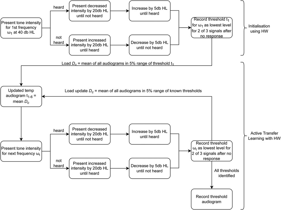
Figure 4. Algorithm for ATL with HW.

4 Results

We used a Dell Laptop computer with an Intel(R) Core(TM) i5-8265U CPU 1.6GHz 1.80GHz. The memory capacity was 8GB. It had a 64-bit Operating System with an x64-based processor running Windows 10 version 2004 (OS Build 19041.1415). The Hard Disk was a 473GB hard drive with 72.2GB of free space.

4.1 Large interaural gaps

The data in the Europe and Central Asia audiogram database had several audiograms with large interaural ranges exceeding 50 dB. Specifically, 926 audiograms had interaural gaps of $\ge 50$ dB, with three audiograms having gaps of 110 dB. In this study, these interaural gaps were allowed. In later studies, a decision can be made to eliminate these gaps as they tend to distort the phenotypes.

4.2 Cleaning up the data

The same database had several incorrect audiogram entries, with one recorded at 510 dB for the 500 Hz frequency and many others recorded strangely as 6, 8, 10, 11 and 12, which we infer could have been incorrect entries for 60, 80, 100, 110 and 120. Other strange values included 66, 81 and 21. These errors seemed as though they were manually inserted, hence introducing human error. These data anomalies were manually deleted as part of the data preparation stage.

The anomalies reveal the importance of preparing data and creating a database with verified and cleaned audiograms. This is important because stream-based active learning is sensitive to such errors.

4.3 Increased phenotypes

We also found that the number of clusters ($k$ ) that could be identified using the k-means clustering method could be increased to 18 clusters, as seen in Figure 3. Nonetheless, we limited the number of clusters to 7 for each database to remain consistent with the WHO standard of seven phenotypes (25) and allowed the combined database to identify 18 clusters (phenotypes).

However, we note that as ML becomes more accessible, the concept of phenotypes might need to be considered as precision audiometry will allow multiple and various types of classifications which might not lend themselves to carefully curated phenotypical classes.

4.4 Accuracy and reliability benchmarks

We present the results of similar studies against which we benchmarked this study. Song et al. (26) performed similar audiogram estimation simulations using Halton samples (low discrepancy sequences that appear random). We use the results from that study to benchmark our simulation results. Tables 4, 5 present the accuracy and reliability results that are used to benchmark our results.

Table 4

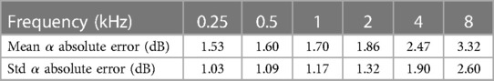
Table 4. Accuracy and reliability for 200 Halton samples in Song (26).

Table 5

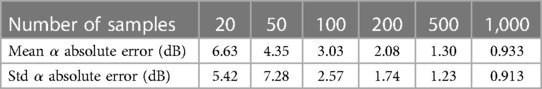
Table 5. Accuracy and reliability of different Halton sample sizes in Song (26).

Song et al.’s (3) experiments with 21 participants gave 78.4 stimuli presentations $\pm 11$ dB for both ears. Table 6 presents their results.

Table 6

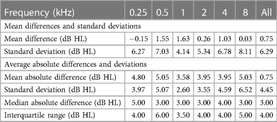
Table 6. Accuracy and reliability for 21 participants in Song (26).

Barbour et al.’s (27) experiments on 21 participants using the same methods of Song et al. (3) implemented in an online platform yielded a mean absolute difference between thresholds of 3.2 presentations $\pm 5.15$ dB. Heisey et al. (28) use a modified version of Song et al. (3) for a mean absolute difference between masked and unmasked experiments of under 5 dB at all frequencies with an overall mean of 3.4 presentations $\pm 2.7$ dB.

4.5 Simulations of HW and ATL

We performed ATL on randomly selected sets of 2, 5, 20, 56 and 556 audiograms from each of the 18 phenotypes identified in the combined audiogram database. This gave 36, 90, 360, 1,008 and 10,008 simulations, respectively. Table 7 shows the mean, standard deviation, minimum, maximum and mode number of stimuli presentations for the simulations of 36 audiograms. Table 8 shows the results for the counts, and Tables 9–13 shows the accuracy and reliability results for the different simulations.

Table 7

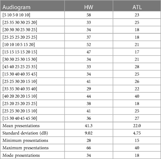
Table 7. Stimuli presentations for the simulation of 36 audiograms (15 examples are shown).

Table 8

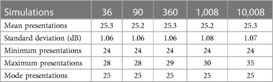
Table 8. Stimuli presentations for the different audiogram simulations.

Table 9

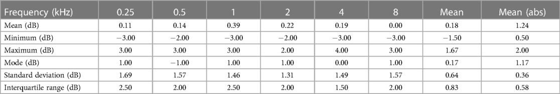
Table 9. Accuracy and reliability for 36 simulations.

Table 10

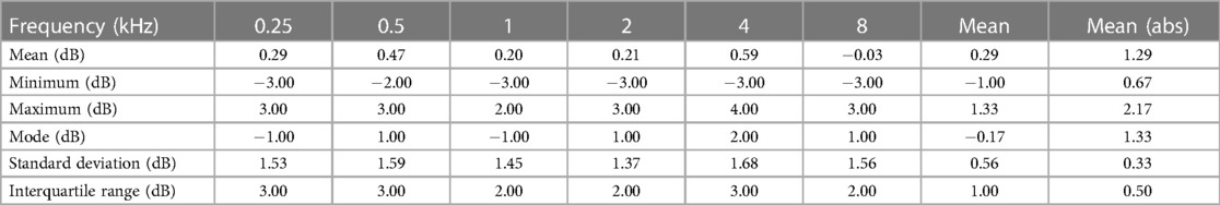
Table 10. Accuracy and reliability for 90 simulations.

Table 11

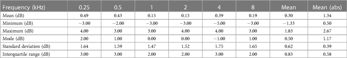
Table 11. Accuracy and reliability for 360 simulations.

Table 12

Table 12. Accuracy and reliability for 1,008 simulations.

Table 13

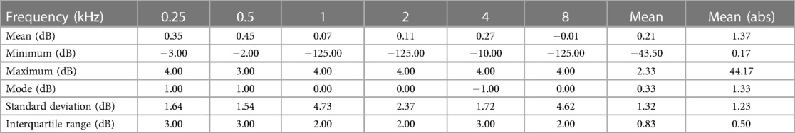
Table 13. Accuracy and reliability for 10,008 simulations.

ATL had lower stimuli presentation variability compared with HW (Table 7) as seen in the improved lower mean of 22.0 presentations with a reliability using standard deviation of $\pm 4.75$ dB. The result is also lower than Song et al. (3) with an average of 78.4 presentations $\pm 11$ dB for both ears, which, when halved, is 39.2 presentations. ATL also had a lower minimum stimuli presentation of 15 compared with the HW minimum count of 28 (Table 7), while for the different simulations between 90 to 10,008, ATL had a minimum stimuli presentation of $25.2\pm 1.06$ dB and a maximum of $25.3\pm 1.06$ dB.

The ATL accuracy was evaluated using the non-parametric numerical 50% probability point from the mean difference and mean absolute difference (Tables 9–13). Reliability was measured using the 25–75% interquartile range (29). The results reveal that ATL accurately determined the threshold at each frequency with very small margins of error of less than 5 dB. ATL was also consistent with much less volatility in its results across all the frequencies also giving a spread of less than 5 dB as well. Even with the simulation of 10,008 audiograms where some of the minimums were more than 125 dB, the spread was still less than 5 dB.

5 Discussion and conclusions

We investigated the influence of informative priors derived from audiogram databases of diverse populations, with an emphasis placed on understanding the degree to which these informative priors can improve CA models without losing computational performance. Specifically, we hypothesized that TL could offer informative priors that improve the accuracy of probabilistic CA models.

The key finding was that Transfer Learning offers an appropriate means to combine audiogram databases to extract meaningful informative priors that can be used in CA. The finding answers Wasmann et al.’s (2) suggestion to find ways to maximise the disparate audiogram databases from around the world.

We offer ATL as a reliable and consistent approach to leverage audiograms from multiple databases to speed up audiogram estimation, in this study improving HW tests from a mean 41.3 presentations $\pm 9.02$ dB down to 25.3 presentations $\pm 1.04$ dB. The reliability and time improvements were also better compared to other existing CA models.

We also found that different population groups have different phenotypes, and therefore are unlikely to share computational parameters or hyperparameters. This means that CA methods on audiogram estimation are likely to become more data-driven compared with being model-driven.

ML methods also produced a varying number of phenotypes from each population according to the data in the dataset. Further research with other ML methods should look into this.

This use of TL to speed audiogram estimation is heavily dependent on the cleanliness of the data. It reveals the importance of preparing data and the necessity to create a database with verified clean audiograms. One of the ways of achieving this is through automating data capture of audiogram records.

We defined an approach as to when to transfer in TL; which is one of the primary problems in TL (14). We also identified what to transfer; the intensity of adjacent frequencies using an exploration mechanism derived from active learning. We then identified the how to transfer using an algorithm which uses any identified intensity in one frequency to predict the intensity in the adjacent frequencies.

5.1 Limitations

We did not cater for imbalanced datasets and hence greater accuracy can be achieved by incorporating algorithms that take into account the imbalances in the datasets. For example, data from Malawi was limited, that is, it had only 400 audiograms.

5.2 Areas for further research

The $k$ number of clusters was intentionally limited to seven for the individual databases in accordance with the WHO recommended number of phenotypes (25). However, the GMM cluster evaluation using k-means clustering yielded up to 18 clusters from the combined audiogram database. This shows, similar to Parthasarathy et al. (15) who identified 10 clusters in their data, that further research can be attempted with a higher number of phenotypes for higher precision. This also brings into question the notion of human audiogram phenotypes considering that ML methods are only getting more advanced. We also found that ATL is sensitive to negative thresholds and tends to overshoot. This phenomenon needs to be investigated further. We also propose that ATL could be extended to other population databases, to include SNHL audiograms, and to include additional information such as altitude and noise exposure.

Data availability statement

The original contributions presented in the study are included in the article/Supplementary Material, further inquiries can be directed to the corresponding author.

Author contributions

HT: Conceptualization, Data curation, Investigation, Software, Writing – original draft. HM: Conceptualization, Resources, Supervision, Writing – review & editing. DLB: Conceptualization, Methodology, Validation, Writing – review & editing.

Funding

The author(s) declare that no financial support was received for the research, authorship, and/or publication of this article.

Conflict of interest

The authors declare that the research was conducted in the absence of any commercial or financial relationships that could be construed as a potential conflict of interest.

Publisher's note

All claims expressed in this article are solely those of the authors and do not necessarily represent those of their affiliated organizations, or those of the publisher, the editors and the reviewers. Any product that may be evaluated in this article, or claim that may be made by its manufacturer, is not guaranteed or endorsed by the publisher.

References

1. WHO. Deafness, hearing loss (2021). (accessed December 9, 2021).

2. Wasmann JW, Lanting C, Huinck W, Mylanus E, van der Laak J, Govaerts P et al. Computational audiology: new approaches to advance hearing health care in the digital age. Ear Hear. (2021) 42:1499–507. doi: 10.1097/AUD.0000000000001041

PubMed Abstract | Crossref Full Text | Google Scholar

3. Song XD, Wallace BM, Gardner JR, Ledbetter NM, Weinberger KQ, Barbour DL. Fast, continuous audiogram estimation using machine learning. Ear Hear. (2015) 36:e326–35. doi: 10.1097/AUD.0000000000000186

PubMed Abstract | Crossref Full Text | Google Scholar

4. Gardner JR, Weinberger KQ, Malkomes G, Barbour D, Garnett R, Cunningham JP. Bayesian active model selection with an application to automated audiometry. Adv Neural Inf Process Syst. (2015) 28:1–9.

Google Scholar

5. Barbour DL, DiLorenzo JC, Sukesan KA, Song XD, Chen JY, Degen EA et al. Conjoint psychometric field estimation for bilateral audiometry. Behav Res Methods. (2019) 51:1271–85. doi: 10.3758/s13428-018-1062-3

PubMed Abstract | Crossref Full Text | Google Scholar

6. Ilyas M, Othmani A, Nait-ali A. Auditory perception based system for age classification, estimation using dynamic frequency sound. Multimed Tools Appl. (2020) 79:21603–26. doi: 10.1007/s11042-020-08843-4. (accessed: February 15, 2021).

Crossref Full Text | Google Scholar

7. Schlittenlacher J, Turner RE, Moore BCJ. Audiogram estimation using bayesian active learning. J Acoust Soc Am. (2018) 144:421–30. doi: 10.1121/1.5047436

PubMed Abstract | Crossref Full Text | Google Scholar

8. van Zyl M, Swanepoel DW, Myburgh HC. Modernising speech audiometry: using a smartphone application to test word recognition. Int J Audiol. (2018) 57:561–9. doi: 10.1080/14992027.2018.1463465

PubMed Abstract | Crossref Full Text | Google Scholar

9. Charih F, Bromwich M, Mark AE, Lefrançois R, Green JR. Data-driven audiogram classification for mobile audiometry. Sci Rep. (2020) 10:1–13. doi: 10.1038/s41598-020-60898-3

PubMed Abstract | Crossref Full Text | Google Scholar

10. Musiek FE, Shinn J, Chermak GD, Bamiou DE. Perspectives on the pure-tone audiogram. J Am Acad Audiol. (2017) 28:655–71. doi: 10.3766/jaaa.16061

PubMed Abstract | Crossref Full Text | Google Scholar

11. Zakaria M. The limitations of pure-tone audiometry (as the gold standard test of hearing) that are worthy of consideration. Indian J Otol. (2021) 27:1. doi: 10.4103/indianjotol.indianjotol-11-21

Crossref Full Text | Google Scholar

12. Cox M, de Vries B. A gaussian process mixture prior for hearing loss modeling. In: Duivesteijn W, Pechenizkiy M, Fletcher GHL, editors. Proceedings of the Twenty-Sixth Benelux Conference on Machine Learning. Technische Universiteit Eindhoven, Netherland: Benelearn (2017). p. 74–6.

13. Zhao Y, Li J, Zhang M, Lu Y, Xie H, Tian Y et al. Machine learning models for the hearing impairment prediction in workers exposed to complex industrial noise: a pilot study. Ear Hear. (2019) 40:690–9. doi: 10.1097/AUD.0000000000000649

PubMed Abstract | Crossref Full Text | Google Scholar

14. Yang Q, Zhang Y, Dai W, Pan S, Transfer Learning. Cambridge, United Kingdom: Cambridge University Press (2020).

15. Parthasarathy A, Romero Pinto S, Lewis RM, Goedicke W, Polley DB. Data-driven segmentation of audiometric phenotypes across a large clinical cohort. Sci Rep. (2020) 10:1–12. doi: 10.1038/s41598-020-63515-5

PubMed Abstract | Crossref Full Text | Google Scholar

16. Charih F, Bromwich M, Lefrançois R, Mark AE, Green JR. Mining audiograms to improve the interpretability of automated audiometry measurements. In: 2018 IEEE International Symposium on Medical Measurements, Applications, Proceedings. Rome, Italy: IEEE (2018). doi: 10.1109/MeMeA.2018.8438746.

17. Martin F, Clark J, Introduction to Audiology. 11th ed. New York, USA: Pearson (2012).

18. Maltby M, Occupational Audiometry. London, United Kingdom: Routledge (2007). doi:10.4324/9780080495378.

19. Alpaydin E, Introduction to Machine Learning (Adaptive Computation, Machine Learning). London, England: The MIT Press (2010).

20. Bishop CM, Pattern Recognition and Machine Learning (Information Science and Statistics). Vol. 128. 1st ed. New York, USA: Springer Science & Business Media B.V. (2006). p. 1–100.

21. Tibshirani R, Walther G, Hastie T. Estimating the number of clusters in a data set via the gap statistic. J R Stat Soc Ser B: Stat Methodol. (2001) 63:411–23. doi: 10.1111/1467-9868.00293

Crossref Full Text | Google Scholar

22. Tong S. Active Learning: Theory and Applications (Ph.D. thesis). Stanford University (2001).

23. Daum H. Frustratingly easy domain adaptation. In: Proceedings of the 45th Annual Meeting of the Association of Computational Linguistics. Prague, Czech Republic: Association for Computational Linguistics (2007). p. 256–63.

24. Gelfand S, Essentials of Audiology. 4th ed. New York, USA: Thieme Medical Publishers, Inc (2016).

25. WHO. World report on hearing (2021). (accessed: June 19, 2023).

26. Song XD, Garnett R, Barbour DL. Psychometric function estimation by probabilistic classification. J Acoust Soc Am. (2017) 141:2513–25. doi: 10.1121/1.4979594

PubMed Abstract | Crossref Full Text | Google Scholar

27. Barbour DL, Howard RT, Song XD, Metzger N, Sukesan KA, DiLorenzo JC et al. Online machine learning audiometry. Ear Hear. (2019) 40:918–26. doi: 10.1097/AUD.0000000000000669

PubMed Abstract | Crossref Full Text | Google Scholar

28. Heisey K. Joint Estimation of Perceptual, Cognitive, and Neural Processes (Ph.D. thesis). Washington University in St. Louis (2020). doi: 10.7936/zssf-hg81.

29. Mahomed F, Swanepoel DW, Eikelboom RH, Soer M. Validity of automated threshold audiometry: a systematic review and meta-analysis. Ear Hear. (2013) 34:745–52. doi: 10.1097/01.aud.0000436255.53747.a4

PubMed Abstract | Crossref Full Text | Google Scholar