Reinforcement learning for path planning of free-floating space robotic manipulator with collision avoidance and observation noise

This study introduces a novel approach for the path planning of a 6-degree-of-freedom free-floating space robotic manipulator, focusing on collision and obstacle avoidance through reinforcement learning. It addresses the challenges of dynamic coupling between the spacecraft and the robotic manipulator, which significantly affects control and precision in the space environment. An innovative reward function is introduced in the reinforcement learning framework to ensure accurate alignment of the manipulator’s end effector with its target, despite disturbances from the spacecraft and the need for obstacle and collision avoidance. A key feature of this study is the use of quaternions for orientation representation to avoid the singularities associated with conventional Euler angles and enhance the training process’ efficiency. Furthermore, the reward function incorporates joint velocity constraints to refine the path planning for the manipulator joints, enabling efficient obstacle and collision avoidance. Another key feature of this study is the inclusion of observation noise in the training process to enhance the robustness of the agent. Results demonstrate that the proposed reward function enables effective exploration of the action space, leading to high precision in achieving the desired objectives. The study provides a solid theoretical foundation for the application of reinforcement learning in complex free-floating space robotic operations and offers insights for future space missions.

1 Introduction

Space exploration represents a sign of human curiosity that drives scientific and technological advancements at the frontier of our knowledge. Space technologies have materialized our wildest dreams, from the exploration of space to the potential colonization of different planets. Among these technologies, robotic manipulators designed for space operations have emerged as critical tools for various missions, including on-orbit servicing, space debris removal, and in-space assembly of large structures due to their high technological readiness level (Papadopoulos et al., 2021). These manipulators perform tasks that would be too dangerous, costly, or time-consuming for human astronauts to perform (Flores-Abad et al., 2014).

Research in space robotic manipulator divides into two distinct categories: free-flying and free-floating (Dubowsky and Papadopoulos, 1993). Free-flying manipulators are characterized by the active control of position and orientation (attitude) of the base spacecraft through the use of thrusters, while the manipulator executes its designated tasks (Seddaoui et al., 2021). This approach, which is analogue to the operation of a fixed-base manipulator, has been extensively studied with focus on path planning and control (Pfeiffer, 1968; Wang et al., 2021). However, the reliance on the thrusters for pose (position and attitude) control incurs significant fuel consumption, potentially reducing the operational lifespan of the system in orbit.

Conversely, free-floating manipulator systems operate with a base spacecraft whose pose is not actively controlled. Instead, the pose of the spacecraft is allowed to naturally react to the manipulator’s joint movements due to the conservation of momentum (Ratajczak and Tchon, 2021; Tsiotras et al., 2023). Intuitively, this approach offers significant advantages, such as the saving of spacecraft fuel and a reduced risk of collision with targets, which might otherwise result from the active attitude control of the base spacecraft. Despite these advantages, controlling free-floating space robots represents a significant challenge. The dynamic interaction between the manipulator and its base spacecraft, due to the conservation of momentum, introduces a complex coupling effect. This effect significantly complicates path planning and motion control, as actions performed by the manipulator can inadvertently after the pose of the base spacecraft, and vice versa. The determination of the pose of the end-effector of the manipulator depends not only on the current joint angles on the manipulator but also on the previous velocities of both the joints and the base spacecraft (Nanos and Papadopoulos, 2017). Additionally, the nonholonomic nature of angular momentum further complicates control strategies, making traditional path-planning solutions, typically used for fixed-base manipulators, ineffective for free-floating space manipulators (Rybus et al., 2017; Dai et al., 2022), highlighting the need for innovative solutions in this area.

2 Related works

To bridge the research gap in the control and path planning of free-floating space manipulator, a challenge not encountered with fixed-base manipulators, various techniques have been proposed (Agrawal et al., 1996; Luo et al., 2018). Early efforts, as outlined in (Agrawal et al., 1996) applied inverse kinematics to path planning while respecting the nonholonomic constraints of angular momentum. However, this approach has limitations in guaranteeing path optimality, as dynamic singularities, which are often unpredictable uniquely from the manipulator’s kinematics, can adversely affect the manipulator’s performance (Xu et al., 2011). In response to these limitations, more recent studies have turned to optimization theory to enhance path-planning solutions, such as particle swarm optimization (Wang et al., 2015) and non-singular terminal sliding mode control (Shao et al., 2021). Despite their promise, these optimization-based solutions often demand substantial computational resources, complicating their application in real-time implementation, especially when facing uncertain disturbances. Additionally, any changes in the initial conditions of the manipulator or its target pose necessitate a comprehensive re-optimization process.

To address this shortfall, researchers have explored the potential of using machine learning (Ye et al., 2019), and more specifically, reinforcement learning (RL), to overcome these limitations (Xie et al., 2020). In essence, RL employs an agent that learns a decision-making policy dynamically through trial-and-error interactions with its environment (in this case, the space manipulator) to maximize a predefined reward function (Sutton and Barto, 2018; Nguyen and Hung, 2019). This learning process, which is within a Markov Decision Process framework, allows the agent to issue commands to alter the environment state and receive feedback in the form of rewards based on the efficacy of its actions. Remarkably, this process does not rely on prior data samples or predefined rules. Hence, the motivation behind exploring the application of RL in tasks like capturing a target by a free-floating space manipulator system lies in its ability to navigate the complexities of the task easily while operating within the constraints of space-based environments. After the training phase concludes, the trained agent is encapsulated solely by a set of weights and biases, represented within neural networks. These parameters are lightweight and can be readily deployed on various hardware platforms without necessitating extensive computational resources. This characteristic is particularly advantageous in space missions where acquiring powerful computational resources is inherently challenging.

Several RL techniques, such as the Deep Deterministic Policy Gradient (DDPG), Actor-Critic algorithm, and Q-learning, have proven effective in path planning for manipulator operating in continuous action spaces. For instance, a study implemented soft Q-learning for path planning of a 3-DOF (Degrees of Freedom) space robotic manipulator (Yan et al., 2018). The reward function in this study was designed based on the distance between the end-effector of the manipulator and the target. It returns positive rewards for minimizing the distance and imposing penalties (negative rewards) for cumulative joint torques.

While the value-based Q-learning performs well when agents select actions from a finite set, policy-gradient based methods like DDPG excel for continuous state and action spaces (Liu and Huang, 2021). In another instance, the DDPG algorithm was applied to path planning for a simple 2-DOF space manipulator (Hu et al., 2018). The reward function in the study included terms for obstacle avoidance, penalties for disturbances from the base spacecraft, and a small penalty for the path length. Additionally, DDPG was used to enhancing the training efficiency of a 3-DOF space robotic manipulator through pre-training (Du et al., 2019). Similarly, a dual-arm space robotic manipulator, each arm with 4-DOF, was trained using DDPG, with the reward function incorporating velocity constraints and penalties to prevent collisions between the arms (Li Haoxuan et al., 2021). Furthermore, the Actor-Critic algorithm was utilized for path planning for a 6-DOF space robotic manipulator, aiming for position and orientation alignment (Liang et al., 2021). The reward function in this case was based not only on the distance difference but also a term for the Euler angle difference between the end effector and the target. In a separate context, DDPG was applied for collision-free path planning for a fixed-base manipulator with 7-DOF, using artificial potential fields within the reward functions to represent obstacles (Li Yinkang et al., 2021). The same algorithm was later applied to a redundant 7-DOF manipulator in a free-floating condition, aiming for target capture with a reward function also based on artificial potential fields (Li et al., 2022).

Table 1 summarizes the current state of RL applications in path planning for space robotic manipulators. This emerging field has seen limited publications to date. The majority of research has focused on training 3-DOF space manipulators, with fewer studies exploring 6-DOF or higher. A significant oversight in many studies in the neglect of joint velocity limitations. Movover, there is a lack of incorporation of quaternion-based expressions for attitude control and consideration of obstacle avoidance in path planning, both of which are crucial for practical applications. Additionally, the use of scalar reward functions in the Markov Decision Process can potentially restrict the search space or result in local optima if not designed with caution. The challenge of balancing exploration-exploitation in RL continues to be a prominent area of research (Jepma and Sander, 2011).

Table 1

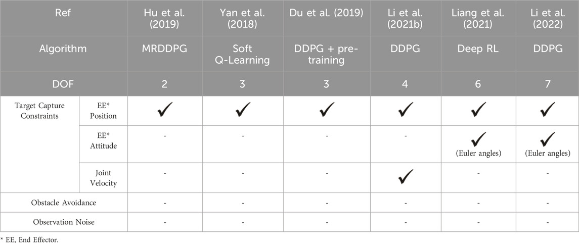
Table 1. Summary of current research on RL-based path planning for space manipulators.

The development of RL path planning in free-floating space manipulators remains scarce. Research suggests that constructing an effective reward function capable of optimizing the control strategy of an agent in a perturbed environment is still a significant challenge.

This paper proposes a deep RL algorithm that integrates DDPG and Actor-Critic neural networks for efficient path planning for a 6-DOF free-floating space manipulator. Our methodology aims to expedite training convergence in dynamic settings by designing reward functions that consider several critical factors. These include aligning the manipulator’s end effector (EE) with the target using a novel quaternion-based approach for orientation comparison and incorporating joint velocity constraints to achieve smoother EE trajectories. Additionally, our algorithm introduces measures to prevent self-collision of the manipulator’s links and, importantly, incorporates external obstacle avoidance capabilities during target approach - a novel feature not previously implemented in the literature. Recognizing the imperfection of real-world sensors, we further enhance our model’s practical applicability by including white noise in the observations during training. This ensures that the trained agent is resilient to signal noise and capable of achieving successful target capture. The effectiveness and advantages of our proposed algorithm are validated through numerical simulations.

3 Mathematic model of a free-floating space manipulator

A general free-floating space robotic manipulator is composed of an n-DOF manipulator mounted on a floating base spacecraft, as shown in Figure 1. An inertial reference frame, designated as OXYZ, is defined in space. Within this frame, the base spacecraft (B₀) is treated as link 0 with 6-DOF and the first link of the manipulator is affixed to the base spacecraft at joint J₁. The manipulator itself is constructed from n rigid links connected in series by n independently actuated revolute joints. The position of the EE is denoted by a vector ${\mathit{p}}_e\in {\mathbb{R}}^3$.

Figure 1

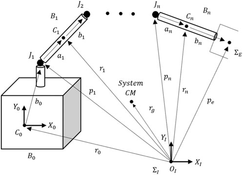
Figure 1. Schematic of a general free-floating space robotic manipulator with n rigid links.

The position (${\mathit{p}}_e$) and orientation (${\mathit{A}}_e$) of the EE can be accurately determined by propagating the relative position and orientation of each joint from the base spacecraft to the end-effector, such that

${\mathit{p}}_e={\mathit{r}}_0+{\mathit{b}}_0+{\displaystyle \sum _{i=1}^n}\left({\mathit{p}}_{i+1}-{\mathit{p}}_i\right)(1)$

${\mathit{A}}_e={\mathit{A}}_o{\displaystyle \prod _{i=1}^n}{\mathit{A}}_i(2)$

where ${\mathit{p}}_i$ is the position vector of the ith joint in the inertial frame and ${\mathit{A}}_i$ is the rotation matrix of the ith link. Differentiating Eqs 1, 2 with respect to time results in the linear (${\mathit{v}}_e\in {\mathbb{R}}^3$) and angular (${\mathit{\omega }}_e\in {\mathbb{R}}^3$) velocities of the EE, such that

${\mathit{v}}_e={\dot{\mathit{p}}}_e={\mathit{v}}_0+{\mathit{\omega }}_0\times \left({\mathit{p}}_e-{\mathit{r}}_0\right)+{\displaystyle \sum _{i=1}^n}\left[\left({\dot{\phi }}_i{\mathit{j}}_i\right)\times \left({\mathit{p}}_e-{\mathit{p}}_i\right)\right](3)$

${\mathit{\omega }}_e={\mathit{\omega }}_0+{\displaystyle \sum _{i=1}^n}{\mathit{\omega }}_i,{\mathit{\omega }}_i={\dot{\phi }}_i{\mathit{j}}_i(4)$

where ${\dot{\phi }}_i$ and ${\mathit{j}}_i$ are the ith joint’s angular velocity and direction in the inertial frame, respectively. Rewriting the velocity equations into a compact matrix form with the base state ${\dot{\mathit{x}}}_b={\left[{\mathit{v}}_0,{\mathit{\omega }}_0\right]}^T$ and EE state ${\dot{\mathit{x}}}_e={\left[{\mathit{v}}_e,{\mathit{\omega }}_e\right]}^T$ yields

${\dot{\mathit{x}}}_e={\mathit{J}}_b{\dot{\mathit{x}}}_b+{\mathit{J}}_m\dot{\mathit{\Phi }}(5)$

where $\dot{\mathit{\Phi }}={\left[{\dot{\phi }}_1,{\dot{\phi }}_2,\cdots {\dot{\phi }}_n\right]}^T$ is the joint angular velocity vector, and (${\mathit{J}}_b$, ${\mathit{J}}_m$) are the Jacobian matrices dependent on the base spacecraft and manipulator motions, respectively.

In a free-floating space manipulator system, the total momentum is conserved. Assuming that the initial momenta of the system is zero, we can express the conservation of momentum conservation as

$\mathit{P}=m_0{\mathit{v}}_0+{\displaystyle \sum _{i=1}^n}{m}_i\left(a_i{\dot{\mathit{p}}}_i+b_i{\dot{\mathit{p}}}_{i+1}\right)=0(6)$

$\mathit{L}=\left({\mathit{I}}_0{\mathit{\omega }}_0+{\mathit{r}}_0\times m_0{\mathit{v}}_0\right)+{\displaystyle \sum _{i=1}^n}\left[{\mathit{I}}_i{\mathit{\omega }}_i+{\mathit{r}}_i\times m_i\left(a_i{\dot{\mathit{p}}}_i+b_i{\dot{\mathit{p}}}_{i+1}\right)\right]=0(7)$

or in the compact matric form as

$\left[\begin{array}{c}\mathit{P}\\ \mathit{L}\end{array}\right]={\mathit{M}}_{\mathit{b}}{\dot{\mathit{x}}}_{\mathit{b}}+{\mathit{M}}_{\mathit{m}}\dot{\mathit{\Phi }}=0(8)$

where $m_i$ is the mass of the ith link, ${\mathit{I}}_i$ is the inertial moment of the ith link at its center of mass (CM), $\left(a_i,b_i\right)$ are fractional coefficients measuring the distances from the CM of the ith link to its two ends and satisfy the condition of $a_i+b_i=1$, ${\mathit{M}}_{\mathit{b}}$ is the inertia matrix of the base spacecraft, and ${\mathit{M}}_{\mathit{m}}$ is the coupling inertia matrix of the manipulator. The detailed expression of these inertia matrices can be found in Wilde et al. (2018).

Combining Eqs. 5, 8 yields

${\dot{\mathit{x}}}_e=\left({\mathit{J}}_m-{\mathit{J}}_b{\mathit{M}}_b^{-1}{\mathit{M}}_{\mathit{m}}\right)\dot{\mathit{\Phi }}={\mathit{J}}_g\dot{\mathit{\Phi }}(9)$

where ${\mathit{J}}_g$ is the generalized Jacobian matrix dependent on the base spacecraft attitude, joint angles, and mass properties of the base and links.

Based on the above kinematics, the dynamics of the free-floating n-link robotic manipulator system, as shown in Figure 1, can be derived by Lagrange equations (Wilde et al., 2018).

$\mathit{M}\ddot{\mathit{q}}+\dot{\mathit{M}}\dot{\mathit{q}}+C\left(\dot{\mathit{q}},\mathit{q}\right)=\mathit{F}(10)$

where

$\mathit{M}=\left[\begin{array}{cc}{\mathit{M}}_b& {\mathit{M}}_{bm}\\ {\mathit{M}}_{bm}^T& {\mathit{M}}_m\end{array}\right]\mathit{F}=\left[\begin{array}{c}\mathbf{0}\\ \mathit{u}\end{array}\right]\mathit{C}=\left[\begin{array}{c}{\mathit{c}}_b\\ {\mathit{c}}_m\end{array}\right]$

and $\mathit{q}={\left[{\mathit{x}}_{\mathit{b}},\mathit{\Phi }\right]}^T$ is the generalized displacement vector of the free-floating space robotic manipulator, ${\mathit{M}}_{bm}$ is the inertia matrix reflecting the dynamic coupling between the base spacecraft and the manipulator, ${\mathit{c}}_b$ and ${\mathit{c}}_m$ represents the Coriolis forces acting on the base spacecraft and the manipulator, and $\mathit{u}$ is the control torque at the joints. This equation serves as the mathematical base in our dynamic simulation environment of a free-floating manipulator, which will be used for reinforcement learning training.

To ascertain the algorithm’s performance and effectiveness under real-world conditions, the parameters used in the simulations are based on actual space robotic manipulator missions (Li et al., 2019). Table 2 shows a brief summary of past space robotic manipulator missions. Notably the mass ratios in most cases are small except for the Orbital Express mission, with a 7.4% mass ratio being the highest. Accordingly, this mass ratio was selected in study to show the need to consider the free-floating base condition.

Table 2

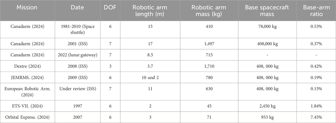
Table 2. Past space robotic capture missions.

4 Reinforcement learning for path planning

4.1 DDPG reinforcement learning algorithm

The control objective of the free-floating manipulator is to move the EE smoothly towards a specified target with precise position and orientation without any collisions between the manipulator’s links, the target, and any obstacles along the path. With this in mind, the observations that are critical to the learning process are defined as

$\mathit{s}=\left[\mathit{\Phi },\dot{\mathit{\Phi }},{\mathit{p}}_e,{\alpha }_e,{\beta }_e,{\gamma }_e,{\dot{\mathit{p}}}_e,{\mathit{\omega }}_e,{\mathit{p}}_T,{\alpha }_T,{\beta }_T,{\gamma }_T,{\dot{\mathit{p}}}_T,{\mathit{\omega }}_T,{\mathit{p}}_{Ob},d,\vartheta \right](11)$

where subscripts “T”, “e”, and “Ob” refer to the target, the end-effector, and Obstacle, respectively, $d$ and $\vartheta$ are the distance and orientation difference between the EE and the target, respectively, to be described in details in Section 4.

The actions that control the manipulator are the torque input at each joint:

$\mathit{a}={\left[u_1,u_2,\cdots ,u_n\right]}^T(12)$

Assuming that the continuous system dynamics between states $\mathit{s}$ and the actions $\mathit{a}$ are discretized in the time domain at time step t_i, we obtain:

${\mathit{s}}_{i+1}=\mathit{f}\left({\mathit{s}}_i,{\mathit{u}}_i,{\mathit{w}}_{\mathit{s},i+1}\right)(13)$

where ${\mathit{u}}_i$ is the control input applied to the system and ${\mathit{w}}_{\mathit{s},i}$ is the noise representing the unmodeled system dynamics in the environment.

Applying RL algorithms, such as Q-learning, to a continuous system like robotic path planning is challenging. This challenge arises from the necessity of optimizing actions ${\mathit{a}}_i$ at each timestep i through a greedy policy. An alternative, the Deep Q-Network (DQN) algorithm (Silver et al., 2014) offers a solution by estimating the Q function with deep neural networks (DNNs) that take states and actions as inputs and return the expected cumulative reward as output. The DQN algorithm uses two distinct DNNs, the main network and target, which operate concurrently. DQN is able to learn value functions using in a stable and robust way due to two innovations (Lillicrap et al., 2015). The network is trained off-policy with samples from a replay buffer to minimize correlations between samples, and the network is trained with a target Q network to give consistent targets during temporal difference backups. This is also used in the DDPG algorithm. Moreover, the response to the input actions by the robotic manipulator is deterministic. Thus, instead of learning a set of probability distributions, a deterministic action can be directly learned from given states for the robotic manipulator system (Silver et al., 2014). Accordingly, the DDPG algorithm is used here to compute the policy gradient $\nabla J\left(\theta \right)$.

The stability of policy gradient methods has been well-studied under the Lyapunov framework. For instance, Hejase and Ozguner, (2023) proved that the policy gradient is negative statistically, which is a crucial factor in ensuring the stability of DDPG methods from a statistical standpoint.

In the DDPG, the actor network deterministically returns in a continuous action space based on its interaction with the environment by the parameterized policy ${\mu }_{{\theta }^Q}$ and is updated by the application of gradient ascent on the policy gradient,

${\nabla }_{\theta }J\left(\theta \right)=\underset{\beta \sim \mu }{\mathrm{E}}\left[{\displaystyle \sum _{i=0}^{N-1}}{\nabla }_{\theta }{\mu }_{\theta }\left({\mathit{a}}_{\mathit{i}}\left|{\mathit{s}}_{\mathit{i}}\right.\right){\nabla }_a{Q}_{{\mu }_{\theta },i}\left({\mathit{s}}_i,{\mathit{a}}_i\right)\right](14)$

where N is the time steps in each episode, $\mu \left(\theta \right)$ is a deterministic policy, and $\beta \left(\theta \right)$ is a behavior policy with different trajectories ${\beta }_{\theta }\left(\left.\mathit{a}\right|\mathit{s}\right)$ from the policy trajectories ${\mu }_{\theta }\left(\left.\mathit{a}\right|\mathit{s}\right)$. The deterministic policy gradient can be calculated by trajectories that are sampled from a distinct behavior policy ${\beta }_{\theta }\left(\left.\mathit{a}\right|\mathit{s}\right)$ based on an Actor-Critic approach (Degris et al., 2012),

$Q_{{\mu }_{\theta },i}\left(\mathit{s},\mathit{a}\right)=\underset{\beta \sim \mu }{\mathrm{E}}\left[{\displaystyle \sum _{i=0}^{N-1}}{\gamma }^i{R}_i\left|\mathit{s}={\mathit{s}}_i,\mathit{a}={\mu }_{\theta }\left({\mathit{s}}_i\right)\right.\right](15)$

Here, $Q_{{\mu }_{\theta }}\left(\mathit{s},\mathit{a}\right)$ is the Q-function that represents the expected discounted return calculated by starting from the ith time step, taking the state-action pair $\left[{\mathit{s}}_i,{\mathit{a}}_i={\mu }_{\theta }\left({\mathit{s}}_i\right)\right]$ and generating rewards based on the policy ${\mu }_{\theta }$ until the end of the episode. Notably, the Q-function depends exclusively on environment, meaning that it can be learned off policy by the Q-learning algorithm (Watkins and Peter, 1992). The parameter $\gamma \in \left[0,1\right]$ is a discount factor. If $\gamma =1$, the agent treats all future rewards equally, which is suitable for long-term planning. On the opposite, the agent is for short-term planning if $\gamma \ll 1$.

The critic network evaluates the agent’s performance by estimating the Q-value of state-action pairs $\left({\mathit{s}}_i,{\mathit{a}}_{\mathit{i}}\right)$. The Q-function is approximated by the Bellman equation (Bellman, 1996).

$Q_{{\mu }_{\theta }}\left({\mathit{s}}_i,{\mathit{a}}_i\right)=\underset{\beta \sim \mu }{\mathrm{E}}\left[R\left({\mathit{s}}_i,{\mathit{a}}_i\right)+\gamma Q_{{\mu }_{\theta }}\left({\mathit{s}}_{i+1},\mu \left({\mathit{s}}_{i+1}\right)\right)\right](16)$

and using Temporal difference, the Q-function can be calculated recursively over a parameter ${\theta }^Q$, to guide the next-generation of actions.

$Q_{{\mu }_{\theta }}^{j+1}\left({\mathit{s}}_i,{\mathit{a}}_i\right)=Q_{{\mu }_{\theta }}^j\left({\mathit{s}}_i,{\mathit{a}}_i\right)+\alpha \left\{\underset{\beta \sim \mu }{\mathrm{E}}\left[R_i\left({\mathit{s}}_i,{\mathit{a}}_i\right)+\gamma {\left.Q_{{\mu }_{\theta }}\left({\mathit{s}}_{i+1},\mu \left({\mathit{s}}_{i+1}\right)\right)\right|}_{{\theta }^Q}\right]-Q_{{\mu }_{\theta }}^j\left({\mathit{s}}_i,{\mathit{a}}_i\right)\right\}(17)$

The critic parameters are updated by reducing the loss function, such that,

$L\left({\theta }^Q\right)=\underset{\beta \sim \eta }{\mathrm{E}}\left[{\left(Q_{{\mu }_{\theta },i}\left({\mathit{s}}_i,{\mathit{a}}_i\left|{\theta }^Q\right.\right)-y_i\right)}^2\right](18)$

$y_i=R_i+{\gamma }^i{Q}_{{\mu }_{\theta },i}\left({\mathit{s}}_{i+1},\mu \left({\mathit{s}}_{i+1}\right)\left|{\theta }^Q\right.\right)(19)$

To ensure the samples are independently distributed, a replay buffer is created to store the tuple $\left({\mathit{s}}_{i+1},{\mathit{s}}_i,{\mathit{a}}_i,R_i\right)$ that are sampled from the environment according to the exploration policy (Lillicrap et al., 2015). At each time step, the actor and critic are updated by sampling a minibatch uniformly from the buffer. When the replay buffer is full the oldest samples are discarded. Because DDPG is an off-policy algorithm, the replay buffer can be large, allowing the algorithm to benefit from learning across a set of uncorrelated transitions.

Directly implementing Q learning with neural networks proved to be unstable in many environments. However, for DDPG the target actor and critic parameters are soft updated, rather than directly copying the weights. The weights of these target networks are updated by having them slowly track the learned networks such that ${\theta }_{Q,i+1}=\tau {\theta }_{Q,i}+\left(1-\tau \right){\theta }_{Q,i+1}$ and ${\theta }_{\mu ,i+1}=\tau {\theta }_{\mu }+\left(1-\tau \right){\theta }_{\mu ,i+1}$ to improve the Q-learning stability, where $\tau \ll 1$ is the smoothing factor (Lillicrap et al., 2015). This means that the target values are constrained to change slowly, greatly improving the stability of learning. This simple change moves the relatively unstable problem of learning the action-value function closer to the case of supervised learning. The pseudo-code that describes the detailed training process for the DDPG algorithm is shown in Table 3.

Table 3

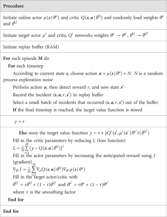
Table 3. Pseudo code of DDPG algorithm.

4.2 Actor-Critic networks

The actor and critic DNNs are created using standard feed-forward neural networks, each one with two hidden layers. The first and second hidden layers have 400 and 300 neurons, respectively. The actor network inputs are the states of the system, and its outputs are the actions. However, the critic network inputs are the state-action pairs, and its outputs are the action values. In this study, the robotic manipulator includes 6 links, i.e., n = 6. Thus, the dimensions of the state and actions are $\mathit{s}\in {\mathrm{S}}^{32}$, and $\mathit{a}\in {\mathrm{A}}^6$, respectively.

4.3 Reward function

As the most critical part of reinforcement learning, the reward function is directly responsible for how the algorithm trains and what objectives are achieved. With that in mind, an innovative reward function is developed to minimize the pose difference between the EE and the target as well as the sudden changes in joint velocities. The reward function ($R_t$) is evaluated at each time step, and the sum of these evaluations across all time steps constitutes the episode reward.

The pose difference is represented by the position error d and the orientation error $\vartheta$. The primary part of the reward function must include:

$R_t=-K_{d}d-K_{\vartheta }\vartheta (20)$

where $K_d$ and $K_{\vartheta }$ are positive reward coefficients. As the pose difference is minimized, the reward $R_t$ is maximized. Notably this guidance term will ensure the agent is learning to align the EE and the target.

The position error is determined straightforward by:

$d=‖{\mathit{p}}_{\mathit{T}}-{\mathit{p}}_e‖=\sqrt{{\left(x_T-x_e\right)}^2+{\left(y_T-y_e\right)}^2+{\left(z_T-z_e\right)}^2}(21)$

The orientation error of the EE can be defined either by a unit quaternion ($\xi$) or a set of Euler angles $\left(\alpha ,\beta ,\gamma \right)$. In the previous work as shown in Table 1, the expression of the orientation error is based on a set of Euler angles, such that,

$\vartheta =\sqrt{{\left({\alpha }_T-{\alpha }_e\right)}^2+{\left({\beta }_T-{\beta }_e\right)}^2+{\left({\gamma }_T-{\gamma }_e\right)}^2}(22)$

where $\left({\alpha }_e,{\beta }_e,{\gamma }_e\right)$ and $\left({\alpha }_T,{\beta }_T,{\gamma }_T\right)$ are the Euler angles of the EE and the target, respectively. It is worth pointing out that the orientation difference in such a form loses the information of rotation sequence of Euler angles. This increases the search space in the learning process and may even lead to divergence. Thus, the Euler angle representation is not used in the current work. Instead, an innovative reward function is built using the quaternion representation of orientations.

Let the orientations of the EE and the target be represented by two unit quaternions ${\xi }_E$ and ${\xi }_T$, respectively, as shown in Figure 2.

Figure 2

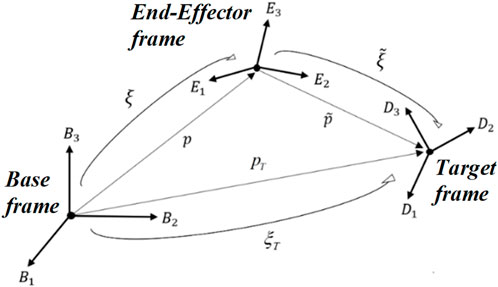
Figure 2. Quaternion representation of orientation difference.

The orientation error of the EE with respect to the target can be expressed as (Campa and Camarillo, 2008):

$\stackrel{\sim }{\xi }={\xi }_T-{\xi }_e={\xi }_T\times {\xi }_e^{*}(23)$

where ${\xi }_e^{*}$ is the conjugate of the quaternion ${\xi }_e$. Accordingly, an orientation difference between the EE and the target is determined by:

$\vartheta =2\arccos \left[\text{Re}\left(\stackrel{\sim }{\xi }\right)\right](24)$

As the EE approaches the desired pose, the pose error ($d$, $\vartheta$) diminishes as well as the reward function in Eq. 20. To ensure the EE stays within the desired pose for capture, large rewards ($r_d$, $r_{\vartheta }$) are added to the reward function in Eq. 20 if $d$ and $\vartheta$ are within predefined ranges, such that:

$R_t=-K_{d}d-K_{\vartheta }\vartheta +r_d+r_{\vartheta }(25)$

$r_d=\left\{\begin{array}{cc}0& \text{if }d\ge d_0\\ r_1& \text{if }d<d_0\end{array}\right.\text{\hspace{1em}and\hspace{1em}}{r}_{\vartheta }=\left\{\begin{array}{cc}0& \text{if }\vartheta \ge {\vartheta }_0\cup d\ge d_0\\ r_2& \text{if }\vartheta <{\vartheta }_0\cap d<d_0\end{array}\right.$

where $d_0$ and ${\vartheta }_0$ are pre-defined indicators for close proximity operation region for position and orientation, respectively. Once the end-effector enters into this region, large positive rewards are assigned to the reward function to encourage and accelerate the agent converging towards the desired pose.

Furthermore, a large negative penalty ($p_l$) is added to the reward function in Eq. 25 to avoid self-collision between the robotic links and the target. If the distance between any two is less than a predefined safe distance, the penalty $p_l$ is added to the reward function, such that:

$R_t=-K_{d}d-K_{\vartheta }\vartheta +r_d+r_{\vartheta }-p_l(26)$

$p_l=\left\{\begin{array}{cc}0& \text{if }\underset{i\ne j}{\min }‖{\mathit{r}}_{\mathit{i}}-{\mathit{r}}_{\mathit{j}}‖\ge r_0\\ p_l& \text{if }\underset{i\ne j}{\min }‖{\mathit{r}}_{\mathit{i}}-{\mathit{r}}_{\mathit{j}}‖<r_0\end{array}\right.$

where $p_l>0$ is a penalty for two links being too close to each other.

To facilitate obstacle avoidance, a substantial negative penalty ($p_{Ob}$) is incorporated into the reward function in Eq. 26. This penalty ($p_{Ob}$) is activated whenever the distance between the obstacle’s CM and any link’s CM falls below a predefined safety range:

$R_t=-K_{d}d-K_{\vartheta }\vartheta +r_d+r_{\vartheta }-p_l-p_{Ob}(27)$

$p_{Ob}=\left\{\begin{array}{cc}0& \text{if }{d}_{Ob}\ge d_{Ob}\\ p_{Ob}& \text{if }{d}_{Ob}<d_{Ob}\end{array}\right.$

Figure 3 shows a simplified illustration of how the safety distance defined between any link and the obstacle is defined.

Figure 3

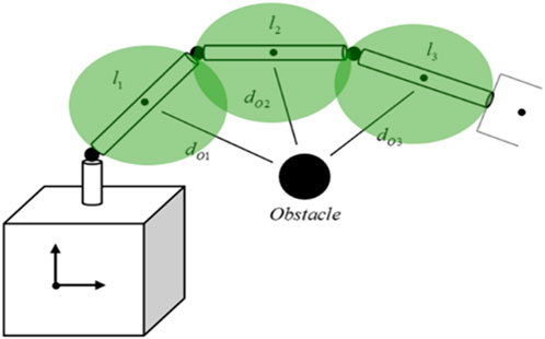
Figure 3. Simplified illustration of obstacle avoidance safety distances.

Finally, in order to ensure a smooth path and avoid sudden changes in motion, a velocity penalty is incorporated as a negative reward ($p_j$) into the reward function described in Eq. 27. This leads to the final reward function R_t,

$R_t=-K_{d}d-K_{\vartheta }\vartheta +r_d+r_{\vartheta }-p_l-p_{Ob}-p_j\sum {\left(\dot{\phi }\right)}^2(28)$

where $p_j>0$ is a velocity penalty for smooth joint velocities by multiplying the squared sum of joint angular velocities.

In summary, the core aspect of RL lies in crafting a robust reward function. The adaptability of our approach shines as we can tailor the reward terms in the reward function to suit varied missions and tasks. This adaptability is evidently demonstrated by the above process to augment the reward function with multiple terms—comprising rewards or penalties—that correspond to the specific objectives at hand. This iterative process ensures our algorithm remains versatile and effective across diverse scenarios.

5 Simulation outcomes and analysis

5.1 Simulation environment

In this study, the proposed RL approach for motion planning of a free-floating space robotic manipulator is verified by simulation using MATLAB^® and Simulink^®. The physical parameters of the manipulator are given in Table 4. Table 5 provides the RL training hyperparameters and the initial conditions for all simulation cases. These simulations were performed on a PC equipped with an Intel^® Core™ i7-10600K Processor and 32 GB of RAM.

Table 4

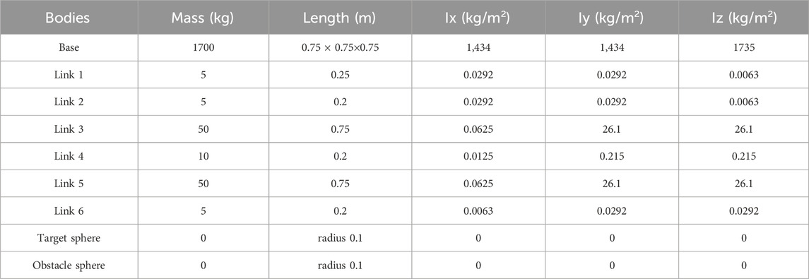
Table 4. Physical parameters of 6-DOF space robotic manipulator (Wilde, et al., 2018).

Table 5

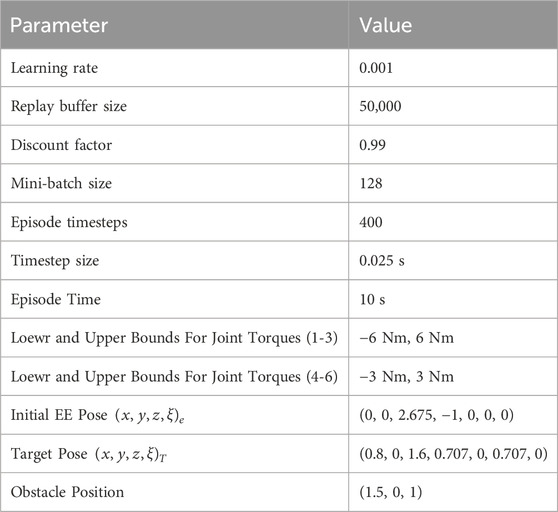
Table 5. RL training hyperparameters and initial conditions.

5.2 Simulation results

Three different cases of path planning were conducted to demonstrate the capabilities of the proposed RL approach, each employing different reward functions. The first case used the reward function in Eq. 27 without velocity constraints. The second case used the reward function in Eq. 28 with the velocity constraints. The third case used the same reward function as the second case. However, it included noisy observations by adding white noise, thereby closely reflecting realistic sensor observations.

5.2.1 Case 1–approach target without velocity constraints

In this case, the free-floating space robotic manipulator has been trained by the reward function in Eq. 27 toward the desired pose ${\left(x,y,z,\xi \right)}_T$. The parameters in this reward function are defined as $k_d=0.1$, $k_{\vartheta }=0.001$, $d_0=0.2m$, ${\vartheta }_0={30}^{\circ }$, $r_d=1$, $r_{\vartheta }=2$, $p_{Ob}=0.5$, $d_{Ob}=0.3$. These parameters are used in all simulation cases described below.

The training progress is shown in Figure 4, where the blue line is the cumulative rewards from all timesteps in each episode, and the red line is the moving average of the cumulative rewards of all episodes. These curves show that the agent learns to reach the desired pose by searching for the highest reward. The term ($-K_{d}d-K_{\vartheta }\vartheta$) in the reward function efficiently guides the EE towards the capture range within the first 5,000 episodes, while the term ($-p_l-p_{Ob}$) in the reward function effectively prevents collisions of the manipulator with the obstacle, the target and itself.

Figure 4

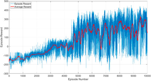
Figure 4. RL training of case 1 for 10,000 episodes.

Upon entering the capture range, the large rewards ($r_d+r_{\vartheta }$) in the reward function are activated to keep the EE within the capture range while simultaneously refining the EE’s pose throughout the remaining timesteps to prepare the gripper for capture. The large variation of the episode reward reflects the activation and deactivation of the large rewards ($r_d+r_{\vartheta }$) in this process. Figure 5 shows several snapshots of the output path for the space robotic manipulator towards the target.

Figure 5

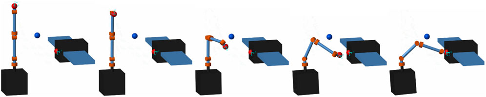
Figure 5. Case 1 solution for space manipulator path reaching the target.

Figure 6A shows the pose error between the EE and the target over time with the left subfigure representing the distance error ($d$) and the right subfigure depicting the orientation difference ($\vartheta$). The trained agent guides the EE towards the desired target pose range ($d_0$, ${\vartheta }_0$) within approximately 6 s. Subsequently, the EE stays within that region to achieve capture for the remaining duration of the simulation. It is worth mentioning that the threshold ($d_0=0.20m$) does not imply that the minimum distance error the trained agent can reach; instead, it signifies that crossing this threshold secures a large positive reward ($r_d$). With this large positive reward, the agent achieves a minimum distance error of Δd = 0.058 m and orientation error of Δθ = 4.85°.

Figure 6

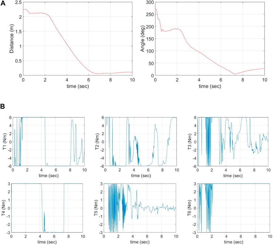
Figure 6. (A) Position and orientation tracking errors vs. time. (B) Time histories of joint torques (actions) given by the agent.

Figure 6B shows the time histories of actions (control torques) at all 6 joints as given by the agent. The agent effectively provides the necessary torques to achieve a valid path for the manipulator to move the EE towards the target, ensuring no self-collision occurs between manipulator links, and most importantly, avoiding the obstacle placed between the EE and the target.

It is worth pointing out that the RL hyperparameters play a pivotal role in governing various aspects of the learning process, including learning dynamics, exploration versus exploitation trade-offs, convergence, adaptation to changing environments, and computational resource utilization. The training is greatly influenced by the learning rate, replay buffer and discount factor. The learning rate dictates the pace at which the RL agent updates its estimates based on new information, influencing both the speed and stability of learning. Similarly, a larger replay buffer enhances sample efficiency and stability by enabling the agent to learn from a diverse array of past experiences while mitigating overfitting risks. Moreover, the discount factor is essential for the agent’s long-term decision-making, allowing it to balance immediate rewards with future gains. This factor significantly influences the convergence and stability of RL algorithms and aids in handling uncertainty and delayed rewards, thus facilitating effective exploration and exploitation strategies.

5.2.2 Case 2–approach target with velocity constraints

To achieve smoother motion and eliminate undesired sudden changes in the path, as shown in Figure 6A at the beginning of the path, often associated with high joint angular velocities, a velocity penalty term for all six joint velocities ($-p_j\sum {\left(\dot{\phi }\right)}^2$) has been added to the reward function, as shown in Eq. 27. The parameters for this simulation case are the same as those in case 1, with the inclusion of an additional parameter of $p_j=0.005$.

The training results are shown in Figures 7, 8. Figure 7 shows the convergence of the reward function. Figure 8A shows the pose error between the EE and the target over time, and Figure 8B shows the time histories of actions (control torques) for all 6 joints given by the agent.

Figure 7

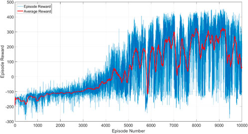
Figure 7. RL training of case 2 for 10,000 episodes.

Figure 8

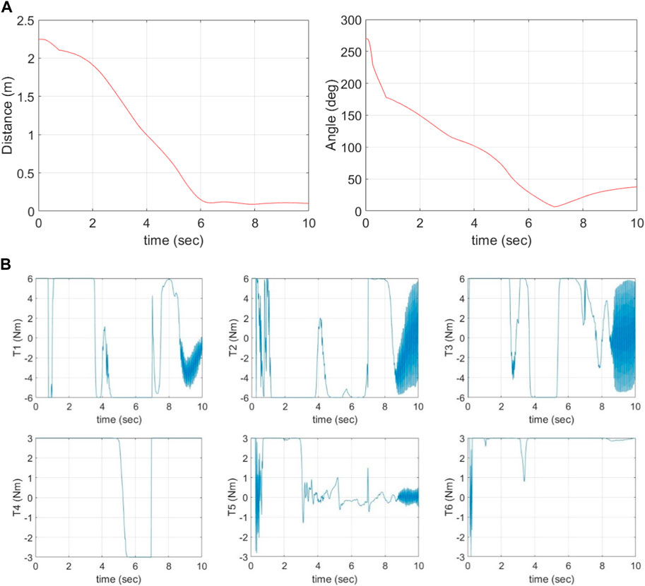
Figure 8. (A) Position and orientation tracking errors vs. time, (B) Time histories of joint torques (actions) given by agent.

In comparison to Figures 4, 7 shows that the training process is similar to Case 1. The training converges to the capture range in approximately 5,000 episodes. Upon entering the capture range, the large rewards ($r_d+r_{\vartheta }$) in the reward function are activated to keep the EE within the capture range while simultaneously refining the EE’s pose throughout the remaining timesteps to prepare the gripper for capture. However, it is noted that in Case 2, the introduction of a velocity penalty term ($-p_j\sum {\left(\dot{\phi }\right)}^2$) to the reward function results in a smoother path. Comparing Figure 8A with Figure 6A reveals an improvement in the convergence of the path in the first 3 s. Furthermore, the end-effector successfully converges towards the capture range. The high rewards ($r_d+r_{\vartheta }$) helps the agent staying in this region for future capture and servicing with a minimum distance error of Δd = 0.088 m and orientation difference of Δθ = 6.61°.

To further examine the effect of the velocity constraint term on agent training, the square sum of all six joint velocities ($\sum {\left(\dot{\phi }\right)}^2$) along the path is shown in Figure 9. It is observed that the square sum of velocities obtained from the path in Case 2 (right plot) barely surpasses 80 in comparison to the 160 reached in Case 1 (left plot). These results clearly demonstrate the efficacy of modifying the reward function on the solution. Such findings open the door for future research to enhance path optimization by designing better reward functions, potentially incorporating torque penalties, energy consumption penalties, and the integration of optimal path constraints commonly used in optimization to RL.

Figure 9

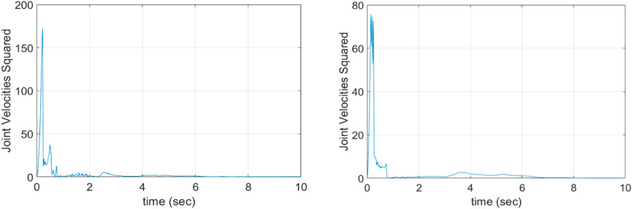
Figure 9. Square sum of all joint angular velocities in Case 1 (left) and Case 2 (right).

5.2.3 Case 3–approach target with noisy observations

In real missions, assuming perfect observations of the state is unrealistic, particularly in estimating the target’s pose using vision sensors like cameras. To evaluate the robustness of the proposed reward function in handling noisy observations, training of the agent was proceeded with the same reward function and parameters in Case 2, except introducing white noise to the observations that would be obtained from cameras in real mission. The noise is added to the target pose and obstacle position: ${\mathit{p}}_T,{\alpha }_T,{\beta }_T,{\gamma }_T,{\mathit{p}}_{Ob}$ with a signal-to-noise ratio (SNR) of 10/1 to simulate realistic conditions:

$Signa{l}_{out}=Signa{l}_{in}\left[1+R_n\right]$

where $R_n\in \left[-0.1,0.1\right]$ is a random number with Mean = 0 and Variance = 1.

The training outcome is shown in Figure 10. It is noted that the agent is able to obtain high rewards despite the presence of observational noise. Figure 11A shows the pose error between the EE and the target over time. Despite the presence of noise in the target position and orientation observations, the agent effectively manages to align the EE and the target for capture. The agent achieves a minimum distance error of Δd = 0.048 m and orientation difference of Δθ = 7.79°. Notably, as the EE approaches the target, the absolute value of the noise decreases, imitating the characteristic behavior observed in real camera observations. The agent successfully overcomes the challenge of noisy inputs, which proves the effectiveness and robustness of the proposed solution.

Figure 10

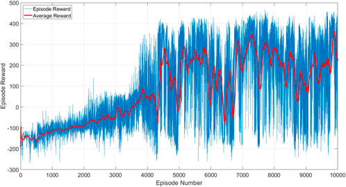
Figure 10. RL training of case 3 for 10,000 episodes.

Figure 11

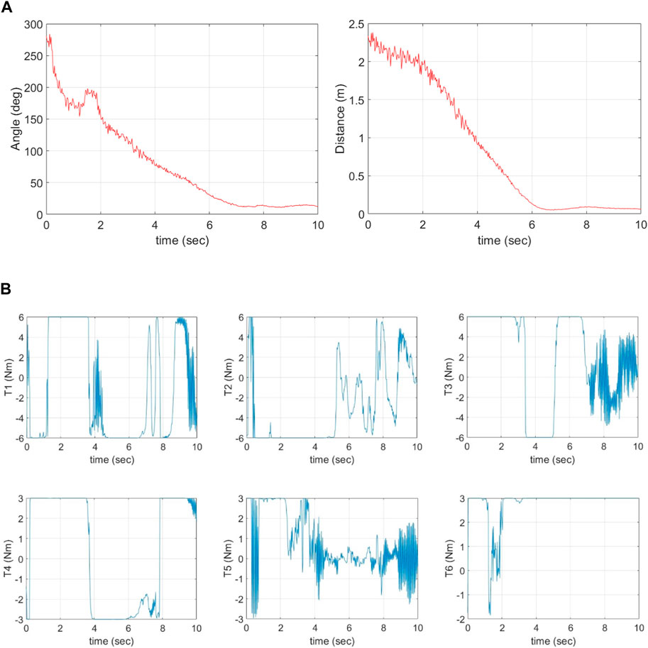
Figure 11. (A) Position and orientation tracking errors vs. time, (B) Time histories of joint torques (actions) given by the agent.

Figure 11B shows the time histories of actions (control torques) for all six joints given by the agent. Observations reveal that the torques required for capture exhibit more oscillations compared to the previous solution in Figure 8. This increase in oscillation results from the noisy observations that add uncertainties during training. It is worth mentioning that the agent trained in Case 3 (noise on observations) still manages to achieve the desired task when implemented in a noise-free environment. Conversely, the agent trained in Case 2 (no noise on observations) fails its task in a noisy environment. This highlights the importance of RL training under realistic and challenging conditions. Exposing the agent to noise during training equips it with the ability to effectively achieve its task in real-world applications.

6 Conclusion

This study investigated the obstacle avoidance path planning problem for a free-floating space robotic manipulator using RL. The DDPG algorithm was used to train an agent to control a 6-DOF space robotic manipulator to achieve the desired goals. Specifically, it aims to find a feasible path towards position and orientation alignment between the EE and the target, without any self-collation between manipulator links, while avoiding external obstacles along the path. The proposed method was verified using simulation with three different simulation cases–without joint velocity constraints, with joint velocity constraints, and with noisy observations. The results show the proper construction of a reward function is critical for training the agent using RL and affects the quality of the path. The inclusion of observation noise in the training will significantly enhance the robustness of the agent. The offline nature of the training in the RL approaches diminishes the need for immediate computational efficiency considerations. After the training phase concludes, the trained agent is encapsulated solely by a set of weights and biases, represented within neural networks. These parameters are lightweight and can be readily deployed on various hardware platforms without necessitating extensive computational resources. This characteristic is particularly advantageous in space missions where acquiring powerful computational resources is inherently challenging.

Data availability statement

The original contributions presented in the study are included in the article/Supplementary material, further inquiries can be directed to the corresponding author.

Author contributions

AA: Conceptualization, Data curation, Formal Analysis, Investigation, Methodology, Software, Validation, Visualization, Writing–original draft, Writing–review and editing. ZZ: Conceptualization, Funding acquisition, Investigation, Methodology, Project administration, Resources, Supervision, Validation, Writing–review and editing, Writing–original draft.

Funding

The author(s) declare that financial support was received for the research, authorship, and/or publication of this article. This work is supported by the FAST grant (19FAYORA14) of the Canadian Space Agency and the Discovery Grant (RGPIN-2018-05991) and CREATE program (555425-2021) of the Natural Sciences and Engineering Research Council of Canada.

Conflict of interest

The authors declare that the research was conducted in the absence of any commercial or financial relationships that could be construed as a potential conflict of interest.

Publisher’s note

All claims expressed in this article are solely those of the authors and do not necessarily represent those of their affiliated organizations, or those of the publisher, the editors and the reviewers. Any product that may be evaluated in this article, or claim that may be made by its manufacturer, is not guaranteed or endorsed by the publisher.

References

Agrawal, S. K., Garimella, R., and Desmier, G. (1996). Free-floating closed-chain planar robots: kinematics and path planning. Nonlinear Dyn. 9, 1–19. doi:10.1007/BF01833290

CrossRef Full Text | Google Scholar

ASC-CSA (2024a). Canadarm, Canadarm2, and Canadarm3 – a comparative table. Available at: https://www.asc-csa.gc.ca/eng/iss/canadarm2/canadarm-canadarm2-canadarm3-comparative-table.asp April 5, 2024).

Google Scholar

ASC-CSA (2024b). Dextre. Available at: https://www.asc-csa.gc.ca/eng/iss/dextre/data-sheet.asp April 5, 2024).

Google Scholar

Bellman, R. (1966). Dynamic programming. Science 153, 34–37. doi:10.1126/science.153.3731.34

PubMed Abstract | CrossRef Full Text | Google Scholar

Campa, R., and Camarillo, K. (2008). Unit quaternions: a mathematical tool for modeling, path planning and control of robot manipulators. Robot. Manip. InTech. doi:10.5772/6197

CrossRef Full Text | Google Scholar

Dai, Ye, Xiang, C., Zhang, Y., Jiang, Y., Qu, W., and Zhang, Q. (2022). A Review of spatial robotic arm trajectory planning. Aerospace 9 (7), 361. doi:10.3390/aerospace9070361

CrossRef Full Text | Google Scholar

Degris, T., White, M., and Sutton, R. S. (2012). Off-policy actor-critic. Available at: https://arxiv.org/abs/1205.4839.

Google Scholar

Du, D., Zhou, Q., Qi, N., Wang, Xu, and Liu, Y. (2019). “Learning to control a free-floating space robot using deep reinforcement learning,” in 2019 IEEE International Conference on Unmanned Systems (ICUS), Beijing, China, October, 2019, 519–523.

CrossRef Full Text | Google Scholar

Dubowsky, S., and Papadopoulos, E. (1993). The kinematics, dynamics, and control of free-flying and free-floating space robotic systems. IEEE Trans. robotics automation 9 (5), 531–543. doi:10.1109/70.258046

CrossRef Full Text | Google Scholar

ETS-VII (2024). ETS-VII. Available at: https://www.eoportal.org/satellite-missions/ets-vii#background-on-ets-missions April 5, 2024).

Google Scholar

European Robotic Arm (2024). European robotic arm. Available at: https://www.esa.int/Science_Exploration/Human_and_Robotic_Exploration/International_Space_Station/European_Robotic_Arm April 5, 2024).

Google Scholar

Flores-Abad, A., Ma, Ou, Pham, K., and Ulrich, S. (2014). A review of space robotics technologies for on-orbit servicing. Prog. Aerosp. Sci. 68, 1–26. doi:10.1016/j.paerosci.2014.03.002

CrossRef Full Text | Google Scholar

Hejase, B., and Ozguner, U. (2023). “Lyapunov stability regulation of deep reinforcement learning control with application to automated driving,” in 2023 American Control Conference (ACC), San Diego, CA, USA, May, 2023, 4437–4442.

CrossRef Full Text | Google Scholar

Hu, X., Huang, X., Hu, T., Zhong, S., and Hui, J. (2018). “Mrddpg algorithms for path planning of free-floating space robot,” in 2018 IEEE 9th International Conference on Software Engineering and Service Science (ICSESS), Beijing, China, November, 2018, 1079–1082.

CrossRef Full Text | Google Scholar

JEMRMS (2024). JEMRMS. Available at: https://iss.jaxa.jp/en/kibo/about/kibo/rms/April 5, 2024).

Google Scholar

Jepma, M., and Sander, N. (2011). Pupil diameter predicts changes in the exploration–exploitation trade-off: evidence for the adaptive gain theory. J. cognitive Neurosci. 23 (7), 1587–1596. doi:10.1162/jocn.2010.21548

PubMed Abstract | CrossRef Full Text | Google Scholar

Li, H., Gong, D., and Yu, J. (2021a). An obstacles avoidance method for serial manipulator based on reinforcement learning and Artificial Potential Field. Int. J. Intelligent Robotics Appl. 5, 186–202. doi:10.1007/s41315-021-00172-5

CrossRef Full Text | Google Scholar

Li, W.-J., Cheng, D.-Yi, Liu, X.-G., Wang, Y.-B., Shi, W.-H., Tang, Z.-X., et al. (2019). On-orbit service (OOS) of spacecraft: a review of engineering developments. Prog. Aerosp. Sci. 108, 32–120. doi:10.1016/j.paerosci.2019.01.004

CrossRef Full Text | Google Scholar

Li, Y., Li, D., Zhu, W., Sun, J., Zhang, X., and Li, S. (2022). Constrained motion planning of 7-DOF space manipulator via deep reinforcement learning combined with artificial potential field. Aerospace 9 (3), 163. doi:10.3390/aerospace9030163

CrossRef Full Text | Google Scholar

Li, Y., Xiaolong, H., She, Y., Li, S., and Yu, M. (2021b). Constrained motion planning of free-float dual-arm space manipulator via deep reinforcement learning. Aerosp. Sci. Technol. 109, 106446. doi:10.1016/j.ast.2020.106446

CrossRef Full Text | Google Scholar

Liang, B., Chen, Z., Guo, M., Wang, Y., and Wang, Y. (2021). Space robot target intelligent capture system based on deep reinforcement learning model. J. Phys. Conf. Ser. 1848 (1), 012078. doi:10.1088/1742-6596/1848/1/012078

CrossRef Full Text | Google Scholar

Lillicrap, T. P., Hunt, J. J., Pritzel, A., Heess, N., Erez, T., Tassa, Y., et al. (2015). Continuous control with deep reinforcement learning. Available at: https://arxiv.org/abs/1509.02971.

Google Scholar

Liu, Y.-C., and Huang, C.-Yu (2021). DDPG-based adaptive robust tracking control for aerial manipulators with decoupling approach. IEEE Trans. Cybern. 52 (8), 8258–8271. doi:10.1109/TCYB.2021.3049555

CrossRef Full Text | Google Scholar

Luo, J., Yu, M., Wang, M., and Yuan, J. (2018). A fast trajectory planning framework with task-priority for space robot. Acta Astronaut. 152, 823–835. doi:10.1016/j.actaastro.2018.09.023

CrossRef Full Text | Google Scholar

Nanos, K., and Papadopoulos, E. G. (2017). On the dynamics and control of free-floating space manipulator systems in the presence of angular momentum. Front. Robotics AI 4, 26. doi:10.3389/frobt.2017.00026

CrossRef Full Text | Google Scholar

Nguyen, H., and Hung, La. (2019). “Review of deep reinforcement learning for robot manipulation,” in 2019 Third IEEE International Conference on Robotic Computing (IRC), Naples, Italy, February, 2019, 590–595.

CrossRef Full Text | Google Scholar

Orbital Express (2024). Orbital express. Available at: https://mda.space/en/orbital-express/April 5, 2024).

Google Scholar

Papadopoulos, E., Aghili, F., Ma, Ou, and Lampariello, R. (2021). Robotic manipulation and capture in space: a survey. Front. Robotics AI 8, 686723. doi:10.3389/frobt.2021.686723

PubMed Abstract | CrossRef Full Text | Google Scholar

Pfeiffer, F. (1986). Manipulator trajectory planning and control. IFAC Proc. Vol. 19 (14), 325–330. doi:10.1016/s1474-6670(17)59499-9

CrossRef Full Text | Google Scholar

Ratajczak, J., and Tchoń, K. (2021). Coordinate-free jacobian motion planning: a 3-d space robot. IEEE Trans. Syst. Man, Cybern. Syst. 52 (8), 5354–5361. doi:10.1109/tsmc.2021.3125276

CrossRef Full Text | Google Scholar

Rybus, T., Seweryn, K., and Sasiadek, J. Z. (2017). Control system for free-floating space manipulator based on nonlinear model predictive control (NMPC). J. Intelligent Robotic Syst. 85, 491–509. doi:10.1007/s10846-016-0396-2

CrossRef Full Text | Google Scholar

Seddaoui, A., Mini Saaj, C., and Nair, M. H. (2021). Modeling a controlled-floating space robot for in-space services: a beginner’s tutorial. Front. Robotics AI 8, 725333. doi:10.3389/frobt.2021.725333

CrossRef Full Text | Google Scholar

Shao, X., Sun, G., Xue, C., and Li, X. (2021). Nonsingular terminal sliding mode control for free-floating space manipulator with disturbance. Acta Astronaut. 181, 396–404. doi:10.1016/j.actaastro.2021.01.038

CrossRef Full Text | Google Scholar

Silver, D., Lever, G., Heess, N., Degris, T., Wierstra, D., and Riedmiller, M. (2014). “Deterministic policy gradient algorithms,” in International conference on machine learning, Beijing, China, June, 2014, 387–395.

Google Scholar

Sutton, R. S., and Barto, A. G. (2018) Reinforcement learning: an introduction. Cambridge, MA, USA: MIT Press, 2–25.

Google Scholar

Tsiotras, P., King-Smith, M., and Ticozzi, L. (2023). Spacecraft-mounted robotics. Annu. Rev. Control, Robotics, Aut. Syst. 6, 335–362. doi:10.1146/annurev-control-062122-082114

CrossRef Full Text | Google Scholar

Wang, L., Lai, X., Meng, Q., and Wu, M. (2021). Effective control method based on trajectory optimization for three-link vertical underactuated manipulators with only one active joint. IEEE Trans. Cybern. 53, 3782–3793. doi:10.1109/tcyb.2021.3125187

CrossRef Full Text | Google Scholar

Wang, M., Luo, J., and Ulrich, W. (2015). Trajectory planning of free-floating space robot using Particle Swarm Optimization (PSO). Acta Astronaut. 112, 77–88. doi:10.1016/j.actaastro.2015.03.008

CrossRef Full Text | Google Scholar

Watkins, C., and Peter, D. (1992). Q-learning. Mach. Learn. 8, 279–292. doi:10.1023/a:1022676722315

CrossRef Full Text | Google Scholar

Wilde, M., Kwok Choon, S., Grompone, A., and Romano, M. (2018). Equations of motion of free-floating spacecraft-manipulator systems: an engineer's tutorial. Front. Robotics AI 5, 41. doi:10.3389/frobt.2018.00041

CrossRef Full Text | Google Scholar

Xie, Z., Sun, T., Kwan, T. H., Mu, Z., and Wu, X. (2020). A new reinforcement learning based adaptive sliding mode control scheme for free-floating space robotic manipulator. IEEE Access 8, 127048–127064. doi:10.1109/ACCESS.2020.3008399

CrossRef Full Text | Google Scholar

Xu, W., Liang, B., and Xu, Y. (2011). Practical approaches to handle the singularities of a wrist-partitioned space manipulator. Acta Astronaut. 68 (1-2), 269–300. doi:10.1016/j.actaastro.2010.07.004

CrossRef Full Text | Google Scholar

Yan, C., Zhang, Q., Liu, Z., Wang, X., and Liang, B. (2018). “Control of free-floating space robots to capture targets using soft q-learning,” in 2018 IEEE International Conference on Robotics and Biomimetics (ROBIO), Kuala Lumpur, Malaysia, December, 2018, 654–660.

CrossRef Full Text | Google Scholar

Ye, X., Dong, Z.-H., and Jia-Cai, H. (2019). Research on adaptive reaction null space planning and control strategy based on VFF–rls and SSADE–ELM algorithm for free-floating space robot. Electronics 8 (10), 1111. doi:10.3390/electronics8101111

CrossRef Full Text | Google Scholar