Design and implementation of high-order PID for second-order processes with time delay

In this study, a state-space pole placement approach is first proposed to design high-order PID controllers for high-order processes. The method makes use of a single parameter to determine the locations of closed-loop poles; thus, a high-order PID controller can be tuned with this parameter. To implement the high-order PID controller in practice, an observer-based PID structure is proposed. The structure utilizes a model-free observer to estimate the plant output and its derivatives, thus retaining the high-order PID structure but can filter the measurement noise and make the high-order derivatives of the plant output available for control. The proposed method is applied to design high-order PID controllers for second-order processes with time delay. Simulation results show that high-order PID can indeed improve the performance of conventional PID controllers for second-order processes with time delay in disturbance rejection and robustness.

1 Introduction

Proportional–integral-derivative (PID) control is the most common feedback control mechanism in the industrial process (Åström and Hägglund, 2001; Chen and Seborg, 2002; Åström and Hägglund, 2006). The reason is that the three parameters of the PID controller have a clear relationship with the performance of the system, so it is easy to tune online. However, with the increase in the complexity of industrial processes and the uncertainties of the controlled plant, the traditional PID control may not meet the requirements of control performance due to its structural characteristics. Some limitations of the PID controller are illustrated in Oliveira et al. (2009). Some techniques are proposed to improve the PID control, including adding integral feedback, feedforward, or delay compensation to the traditional PID loop, which makes the PID structure complicated and requires extra parameters (Duan et al., 2008). On the other hand, control scholars put forward many advanced control methods to replace PID control, such as LQG (Garrido-Moctezuma et al., 1997), H infinity (Tan et al., 2006), and adaptive control (Mocci et al., 2020). Although these advanced control methods improve the control performance, they are rarely used in practice due to implementation, tuning, and maintenance issues. Therefore, more than 90% of the loops in the industrial process still use the PID structure (Dash et al., 2015; Latif et al., 2020).

It is well-known that PI control is suitable for first-order processes and PID control is suitable for second-order processes. For second-order processes with time delays, will high-order PID with a second-order derivative $\left(\mathrm{PID}{\mathrm{D}}^2\right)$ improve the performance of the conventional PID? When the control performance for high-order processes can be improved by increasing the controller order beyond the PID control, there are few literature works investigating how to tune the parameters of high-order PID to enhance the disturbance rejection ability.

Vrančić and Huba, (2021) show that the high-order PID controllers can significantly improve the control performance of various process models. Lin et al. (2021) illustrate that high-order linear active disturbance rejection controllers (LADRCs) can be interpreted as high-order PID with low-pass filters for speed servo systems and position servo systems. Huba et al. (2021) find that high-order PID control enables faster transients by simultaneously reducing the negative effects of measurement noise and increasing the closed-loop robustness. Huba and Vrani (2018) extend the 2DOF PI and PID controller design for the first-order time-delayed plant by the multiple real dominant pole method to the 2DOF $\mathrm{PID}{\mathrm{D}}^2$ control. A novel optimal PID plus second-order derivative controller for the AVR system is proposed by Sahib (2015). An algorithm of optimal settings for high-order PID in ship power plants is proposed with perfect performance (Simanenkov et al., 2017).

In practice, PI controllers are used more often than PID controllers, since the latter significantly increases the controller output noise (Ediga and Ambati, 2021). One reason is that the derivative term is very sensitive to the measurement noise, so an appropriate filter can significantly improve the closed-loop performance (Segovia et al., 2014). Naturally, with higher degrees of controllers, the problem becomes aggravated. Therefore, the appropriate high-order filter is inevitable in practical applications. Furthermore, obtaining derivative and high-order derivative signals may amplify sensor noises. Therefore, the filter is usually considered an integral part of the PID design, and the filter constants need to be selected as a compromise between robustness and performance, so PID tuning is essentially a four-parameter design procedure. However, noise is not considered in high-order PID at present. In view of this, considering the form of the high-order PID controller and ensuring the selection of its adjustable poles should be an improvement way that can be considered. Therefore, a high-order PID design method and noise suppression method are proposed in this study.

In this study, an observer is used to estimate the output and derivative of the system, and a high-order PID control structure is proposed, which does not depend on the controlled plant model and retains the traditional PID control structure but increases the controller’s disturbance rejection ability. Usually, a time delay is an approximation of high-order dynamics of the controlled plant except the pure transport delay. So, a process with time delay is in fact a high-order system; thus, a high-order PID controller can be used to achieve better control performance. The goal of the study was to propose a practical control structure that can utilize high-order derivatives of the process to improve the control performance, as compared with the conventional three-term PID controller, and we tried to design the controller via the modern control method. The structure and the design method can build a link between the modern control theory and classical control theory. The main contributions of this study are as follows: 1) an observer-based PID structure is proposed to improve the performance of conventional PID by providing high-order derivatives. The proposed observer-based PID structure is an extension of the conventional PID + filter structure in which high-order derivatives can be incorporated into the structure and the measurement noise can be handled through the extended state observer. 2) A state-space pole placement method is proposed to directly design PID gains, thus linking the modern control theory with the classical control theory. It retains the essential terms of conventional PID. To obtain a PID controller gain, the trick is to transform the model into the canonical observable form. The method is applied to second-order processes with time delay, and the simulation results show that the structure can achieve better performance than other variations of PID, and the design is in the usual modern control theory framework.

The structural arrangement of this study is as follows: in Section 2, the high-order PID controller is proposed to design through the pole placement method; in Section 3, an observer-based PID is proposed to implement high-order PID in practice; the structure and tuning of high-order PID for a variety of second-order timed-delayed systems are tested in Section 4; finally, conclusions are given in Section 5.

2 Design of high-order PID controllers via pole placement

There are many methods to get the parameters of an ideal PID. It is possible to apply the state feedback design in the PID design which is a convenient and useful control design method in the modern control theory. It is shown that the available plant model information used in the high-order PID design can guarantee the stability of the actual plant. Suppose the controlled plant has a minimal state-space realization as follows:

$\begin{array}{c}\{\begin{array}{c}\dot{x}=Ax+Bu,\\ y=Cx.\end{array}\end{array}(1)$

In this study, we will propose a method to design a high-order PID controller. Our idea is to obtain a state feedback control law $u=Kx$ using the well-known pole-placement method. However, since the state vector x is not necessarily composed of y and its derivatives, $K$ is not a PID control gain. To solve the problem, consider the canonical observable form of the controlled plant which is used to make sure that the state-feedback gain is the PID gain:

$\begin{array}{c}\{\begin{array}{c}\dot{z}=A_{o}z+B_{o}u,\\ y=C_{o}z,\end{array}\end{array}(2)$

where $\mathrm{z}={\left[z_1 z_2 \cdots z_m\right]}^T$ is the state vector, and

$\begin{array}{c}\begin{array}{c}{\text{A}}_o={\left[\begin{array}{ccccc}0& 1& 0& \cdots & 0\\ 0& 0& 1& \cdots & 0\\ ⋮& ⋮& ⋮& \ddots & ⋮\\ 0& 0& 0& \cdots & 1\\ -a_0& -a_1& -a_2& \cdots & -a_{m-1}\end{array}\right]}_{m\times m},{\text{B}}_o={\left[\begin{array}{c}{d}_1\\ d_2\\ d_3\\ ⋮\\ d_m\end{array}\right]}_{m\times 1}, \\ {\overline{C}}_e={\left[\begin{array}{ccccc}1& 0& \cdots & 0& 0\end{array}\right]}_{1\times m},\end{array}\end{array}(3)$

$\begin{array}{c}{A}_o=TA{T}^{-1},B_o=TB,C_o=C{T}^{-1},\end{array}(4)$

where $T$ is a state transformation matrix and the observability matrix of (1). In this canonical form, the state vector $\text{z}$ has a clear physical meaning, and its elements are:

$\{\begin{array}{c}{\dot{z}}_1=z_2+d_{1}u,\\ {\dot{z}}_2=z_3+d_{2}u,\\ ⋮\\ {\dot{z}}_{m-1}=z_m+d_{m-1}u.\end{array}(5)$

Since $\mathrm{y}=z_1$, then

$\{\begin{array}{c}{z}_2={\dot{z}}_1-d_{1}u=\dot{y}-d_{1}u\\ z_3={\dot{z}}_2-d_{2}u=\ddot{y}-d_{1}u-d_{2}u\\ ⋮\\ z_m={\dot{z}}_{m-1}-d_{m-1}u=y^{\left(m-1\right)}-d_1{u}^{\left(m-2\right)}-\cdots d_{m-1}u\end{array}(6)$

Define a new variable $z_{m+1}$ as

$\begin{array}{c}{\dot{z}}_{m+1}=z_1=y\end{array}.(7)$

Here, $z_{m+1}$ is the integral of y, and the extended state-space model of the controlled plant is

$\begin{array}{c}\{\begin{array}{c}\left[\begin{array}{c}\dot{z}\\ {\dot{z}}_{m+1}\end{array}\right]=\left[\begin{array}{cc}{A}_o& 0\\ C_o& 0\end{array}\right]\left[\begin{array}{c}z\\ z_{m+1}\end{array}\right]+\left[\begin{array}{c}{B}_o\\ 0\end{array}\right]u,\\ y=\left[\begin{array}{cc}{C}_o& 0\end{array}\right]\left[\begin{array}{c}z\\ z_{m+1}\end{array}\right].\end{array}\end{array}(8)$

Suppose a state-feedback control law ${\mathrm{K}}_{\mathrm{o}}\mathrm{=}\left[\begin{array}{ccccc}{\mathrm{k}}_{\mathrm{1}}& {\mathrm{k}}_{\mathrm{2}}& \cdots & k_m& {\mathrm{k}}_{\mathrm{m+1}}\end{array}\right]\mathrm{ }$ has been designed for (8), then

$\begin{array}{l}u=k_1+z_1+k_2{z}_2+\cdots +k_m{z}_m+k_{m+1}{z}_{m+1}\\ =k_{1}y+k_2\left(\dot{y}-d_{1}u\right)+\cdots \\ +k_m\left(y^{\left(m-1\right)}-d_1{u}^{\left(m-2\right)}-\cdots -d_{m-1}u\right)+k_{m+1}{\displaystyle {\int }_0^{t}y\left(\tau \right)d\tau .}\end{array}(9)$

To obtain a static state feedback gain with only derivatives and integral of y, by ignoring the derivatives of u, then we have

$\begin{array}{c}u=\frac{k_{1}y+k_2\dot{y}+\cdots +k_m{y}^{\left(m-1\right)}+k_{m+1}{{\displaystyle \int }}_0^{t}y\left(\tau \right)d\tau }{1+{\displaystyle {\sum }_{i-2}^m{k}_i{d}_{i-1}}}\end{array}.(10)$

Here, u is the combination of the derivatives and integrals of y. It is in the form of a high-order PID control, with gain. ${\overline{K}}_o=\frac{\left[\begin{array}{ccccc}{k}_m& \cdots & k_2& k_1& k_{m+1}\end{array}\right]}{1+{\displaystyle {\sum }_{i-2}^m{k}_i{d}_{i-1}}}=:\left[\begin{array}{cccccc}{K}_{d,m-1}& \cdots & K_{d2}& K_d& K_p& K_i\end{array}\right].$

For the second-order system (m = 2), (10) is the conventional PID control, with

$\begin{array}{c}{K}_p=\frac{k_1}{1+k_2{d}_1},K_i=\frac{k_3}{1+k_2{d}_1},K_d=\frac{k_2}{1+k_2{d}_1}\end{array}.(11)$

For the third-order system (m = 3), (10) is $\mathrm{PID}{\mathrm{D}}^{\mathrm{2}}$. A $\mathrm{PID}{\mathrm{D}}^{\mathrm{2}}$ form extends the conventional PID structure with a second-order derivative. Gains have clear physical meaning and are directly related to the performance of the closed-loop system, with

$\begin{array}{c}{K}_p=\frac{k_1}{1+k_2{d}_1+k_3{d}_2},K_i=\frac{k_4}{1+k_2{d}_1+k_3{d}_2},K_d=\frac{k_2}{1+k_2{d}_1+k_3{d}_2}\\ K_{d2}=\frac{k_3}{1+k_2{d}_1+k_3{d}_2}.\end{array}(12)$

The state-feedback law (9) can be designed by the well-known pole-placement method. It is well-known that the dominant poles determine the rise time and damping of the closed-loop system, so they can be used to tune the parameters of high-order PID. To design different-order controllers, different numbers of poles are selected as suggested in (13). The two poles $\left({\text{s}}_1,s_2\right)$ are dominant poles, and others $\left({\text{s}}_i,i=3,\dots ,\mathrm{m}+1\right)$ are located in the same place with a larger real part that is determined by the parameter $\overline{\alpha }$. For example, to design a second-order controller (PID), three poles (a pair of dominant poles + a negative real pole) can be used in the pole-placement method. To design a third-order controller (PIDD²), four poles (a pair of dominant poles + two (same) negative real poles) can be used. For simplicity, the poles can be chosen as:

$\begin{array}{c}{s}_{\mathrm{1,2}}=-{\overline{\omega }}_c\left(\overline{\xi }\pm \sqrt{1-{\overline{\xi }}^{2}j}\right),s_i=-\overline{\alpha }{\overline{\omega }}_c\left(i=3,\cdots ,m+1\right)\end{array}.(13)$

From extensive simulations, in order to have good damping and fast settling time in the disturbance rejection response, the damping ratio $\overline{\xi }$ of the dominant poles can be chosen as 0.8 and $\overline{\alpha }$ can be chosen as 2 for other poles so that the disturbance rejection response has a good damping and fast settling time. So, we need only one parameter ${\overline{\omega }}_c$ to tune the high-order PID gain ${\overline{\mathrm{K}}}_{\mathrm{o}}$.

3 Practical implementation of high-order PID controllers

In the previous section, ideal PID and $\mathrm{PID}{\mathrm{D}}^{\mathrm{2}}$ controllers were designed and tuned. It is well-known that the derivative action is sensitive to measurement noise, so in practice, filters should be used to implement ideal PID and $\mathrm{PID}{\mathrm{D}}^{\mathrm{2}}$ controllers.

In this study, we try to estimate the derivatives of the output via an observer instead of using filters. Consider the ideal $\mathrm{PID}{\mathrm{D}}^{m-\mathrm{1}}$ controller:

$\begin{array}{c}u=K_{p}y+K_d\dot{y}+\cdots +K_{d,m-1}{y}^{\left(m-1\right)}+K_i{\displaystyle \underset{0}{\overset{t}{\int }}y\left(\tau \right)d\tau }\end{array}.(14)$

It can be treated as the state-feedback gain $u={\overline{K}}_{o}x$ for the following state-space model.

$\begin{array}{c}\{\begin{array}{c}\dot{x}={\overline{A}}_{e}x+{\overline{B}}_{e}u,\\ y={\overline{C}}_{e}x,\end{array}\end{array}(15)$

where the state vector is defined as

$\begin{array}{c}x={\left[\begin{array}{ccccc}{y}^{\left(m-1\right)}& \cdots & \dot{y}& y& {\displaystyle \underset{0}{\overset{t}{\int }}y\left(\tau \right)d\tau }\end{array}\right]}^{\mathrm{T}}\end{array}(16)$

and the controller gain is

$\begin{array}{c}{\overline{K}}_o=\left[\begin{array}{ccccc}{K}_{d,m-1}& \cdots & K_d& K_p& K_i\end{array}\right]\end{array},(17)$

and the state-space matrices are

$\begin{array}{c}\begin{array}{c}{\overline{A}}_e={\left[\begin{array}{ccccc}0& 0& \cdots & 0& 0\\ 1& 0& \cdots & 0& 0\\ 0& 1& \cdots & 0& 0\\ ⋮& ⋮& \ddots & ⋮& ⋮\\ 0& 0& \cdots & 1& 0\end{array}\right]}_{\left(m+1\right)\times \left(m+1\right)},{\overline{B}}_e={\left[\begin{array}{c}{b}_0\\ 0\\ 0\\ ⋮\\ 0\end{array}\right]}_{\left(m+1\right)\times 1}\\ {\overline{C}}_e={\left[\begin{array}{ccccc}0& \cdots & 0& 1& 0\end{array}\right]}_{1\times \left(m+1\right)}.\end{array}\end{array}(18)$

The state vector $\left(1\right)$ contains the (high-order) derivatives and integral of $y$. An extended Luenberger observer (Du et al., 2022) can be used to observe the state variables, so the derivatives and integrals of $y$ can be estimated instead of using a filter.

$\begin{array}{c}\dot{\overline{x}}=\left({\overline{A}}_e-{\overline{L}}_o{\overline{C}}_e\right)\overline{x}+{\overline{B}}_{e}u+{\overline{L}}_{o}y\end{array}(19)$

with the observer gain ${\overline{L}}_o$, where

$\begin{array}{c}{\overline{L}}_o={\left[\begin{array}{ccccc}{\overline{\mathrm{\beta }}}_{\mathrm{1}}& {\overline{\mathrm{\beta }}}_{\mathrm{2}}& \cdots & {\overline{\mathrm{\beta }}}_{\mathit{m}}& \mathrm{1}\end{array}\right]}^{\mathrm{T}}\end{array}.(20)$

For simplicity, the observer gain ${\overline{L}}_o$ (20) can be tuned via the bandwidth idea (Gao, 2003). The poles of the observer are all placed at the same location $\left(-{\omega }_o\right)$, so the observer gain can be found from:

$\begin{array}{c}{\overline{\mathrm{\beta }}}_i=C_m^{i-1}{\mathrm{\omega }}_o^{m+1-i}\left(i=1,\dots ,m\right)\end{array},(21)$

when the observer gain is chosen properly, ${\overline{A}}_e-{\overline{L}}_o{\overline{C}}_e$ is asymptotically stable, and

$\begin{array}{c}\begin{array}{c}{\overline{x}}_1\left(t\right)\to y^{\left(m-1\right)}\left(t\right),\cdots ,{\overline{x}}_m\left(t\right)\to y\left(t\right),\\ {\overline{x}}_{m+1}\left(t\right)\to {\displaystyle \underset{0}{\overset{t}{\int }}y\left(\tau \right)d\tau .}\end{array}\end{array}(22)$

Combining the state feedback control and the observer, a state-space realization (mth-order) of $\mathrm{PID}{\mathrm{D}}^{\left(m-1\right)}$ (hereafter, it will be referred to as an observer-based PID (OB-PID)) is obtained as:

$\begin{array}{c}\{\begin{array}{c}\dot{\overline{x}}=\left({\overline{A}}_e-{\overline{L}}_o{\overline{C}}_e\right)\overline{x}+{\overline{B}}_{e}u+{\overline{L}}_{o}y,\\ u={\overline{K}}_o\left(\overline{r}-\overline{x}\right).\end{array}\end{array}(23)$

Note that (23) is a standard state-feedback-observer form; however, the novelty is that the state-feedback gain can be interpreted as the (high-order) PID gain due to the special state-space coefficients, and thus it builds a link between modern control and classical control theories. Not every state-feedback-observer form can be interpreted as this. It is a practical implementation of the ideal $\mathrm{PID}{\mathrm{D}}^{\left(m-1\right)}$ (an extension of traditional PID with high-order derivatives).

The structure of $m$th-order observer-based PID is shown in Figure 1, where the derivatives of the signal $r$ are set to zero for step-like reference and $\mathrm{\alpha }$ is a setpoint weight that can improve the tracking performance significantly by reducing the overshoot for integrating and unstable processes. By default, $\mathrm{\alpha }=1$. Thus, as the pole placement procedure shown in section 2, for $m$th-order observer-based PID, one parameter ${\omega }_c$ (controller bandwidth) can be used to tune ${\overline{K}}_o$ (17) and one parameter ${\omega }_o$ (observer bandwidth) can be used to tune ${\overline{L}}_o$ (20).

FIGURE 1

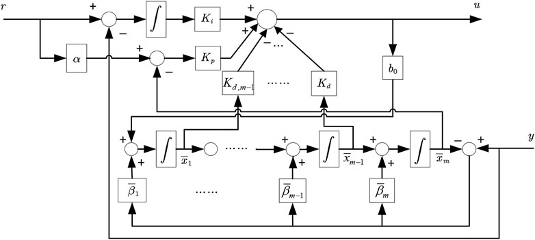
FIGURE 1. Structure of the observer-based PID.

It is noted that the output $y\left(t\right)$ and its derivatives are estimated from the canonical cascaded integral model in $m$th-order observer-based PID:

$\begin{array}{c}{y}^{\left(m\right)}\left(t\right)=b_{0}u\left(t\right)\end{array},(24)$

instead of using the true model. Thus, the model-independent control structure of PID is retained.

$b_0$ is a scaling coefficient of estimation of $y$, which can help reduce the bandwidth of the observer when necessary. This can be verified by the transfer function from $y$ to $u$ of observer-based PID. The proposed design method relies on the order of the system (in fact, on the model of the system), which is not accurately known in a practical system. However, the proposed observer-based PID structure is independent of the detailed model, just like conventional PID. The difference is that the conventional PID is restricted to second-order, while the observer-based PID can be of any order. The order is the information that the designer knows about the controlled plant. For a high-order system, if a first-order model is used to approximate it, then a first-order controller (PI) will be obtained; if a second-order model is used, then a second-order controller (PID) will be obtained; and if a third-order model is used, then a third-order controller (PIDD²) will be obtained. So the order can be chosen by the designer. In this study, we are interested in the PIDD² controller, so a second-order model with time delay (the third-order model) is used in the design. For example, when $m=2$, the feedback controller from $y$ to $u$ becomes

$\begin{array}{c}{K}_c\left(s\right)=\frac{\left(K_d{\beta }_1+K_p{\beta }_2+K_i\right)s^2+\left(K_p{\beta }_1+K_i{\beta }_2\right)s+K_i{\beta }_1}{s\left(s^2+\left({\beta }_2+K_d{b}_0\right)s+\left({\beta }_1+K_p{b}_0+K_d{\beta }_2{b}_0\right)\right)}\end{array},(25)$

when $K_d, K_p, K_i$ and ${\overline{\mathrm{\beta }}}_{\mathrm{1}}\mathrm{,}{\overline{\mathrm{\beta }}}_{\mathrm{2}}$ are fixed, and a small $b_0$ will make the integral gain of $K_c\left(s\right)$ approximate the integral gain $K_i$ of the ideal PID.

4 Simulation

This section verifies the high-order PID design for a variety of second-order processes with time delay. To use the state-space pole placement method, the delay can be approximated using the first-order Pade approximation. As an application of the high-order PID control, we consider disturbance rejection and robustness analysis of different control methods. To measure the robustness of the designed system, the peak of the sensitivity function $\left(M_s=S_{\infty }=\underset{\omega }{\max }\left|\frac{1}{1+L\left(j\omega \right)}\right|\right)$ is used, where $\mathrm{L}\left(\mathrm{s}\right)\mathrm{=G}\left(\mathrm{s}\right)\mathrm{K}\left(\mathrm{s}\right)$ is the open-loop transfer function. It is to be noted that the peak of S usually occurs at low- and mid-frequencies, so $M_s$ is a measure of system robustness against low- and mid-frequency uncertainties. The larger the value of $M_s$, the weaker the robustness and the better the disturbance rejection. Similarly, the smaller the value of $M_s$, the better the robustness and the worse the disturbance rejection performance. Total variations $\left(\mathrm{TV}={\displaystyle \sum _1^{\infty }\left|u_{i+1}-u_i\right|}\right)$ of the control input u(t) for different controllers are also used in this study. They are compromised with pole positions, which are determined by ${\mathrm{\omega }}_{\mathrm{c}}$ in (13) and ${\mathrm{\omega }}_{\mathrm{o}}$ in (21). To evaluate the closed-loop load disturbance attenuation performance, the integral of time and absolute errors (ITAE) is considered, which is defined as:

$\begin{array}{c}\mathrm{I}\mathrm{T}\mathrm{A}\mathrm{E}={\displaystyle \underset{0}{\overset{\infty }{\int }}t\left|e\left(t\right)\right|}dt,\end{array}(26)$

where $\mathrm{e}\left(\mathrm{t}\right)\mathrm{=r}\left(\mathrm{t}\right)-\mathrm{y}\left(\mathrm{t}\right)$. For fair comparisons, in the following simulations, ideal PID is implemented via the practical PID, with the filter time constant Td/N (n = 20) if the references have not given the practical PID form. Also, since the initial response of a PID controller is large without setpoint weighting, while the proposed OB-PID has setpoint weighting, the control signals of the simulations are plotted within a suitable limit to distinguish them from the load disturbance rejection response. The performance indexes, ITAE and TV, are computed only for the load disturbance rejection response.

Example 1. Considering the following second-order plus time delay (SOPTD) process

$\begin{array}{c}{\mathrm{G}}_1\left(s\right)=\frac{e^{-2s}}{\left(s+1\right)\left(0.7s+1\right)}\end{array},(27)$

a high-order PID control can be tuned with ${\omega }_c=0.62$ for ${\overline{K}}_o$, and we can get $\mathrm{PID}{\mathrm{D}}^2$ gain as

$\begin{array}{c}{K}_p=0.7506,K_i=0.3371,K_d=0.5497,K_{d2}=0.1297\end{array}.(28)$

The observer bandwidth ${\overline{\omega }}_o=10$ is chosen for the extended observer gain. Then, a third-order observer-based PID with the following parameters can be obtained:

$\begin{array}{c}{\overline{K}}_o=\left[\begin{array}{cccc}0.1297& 0.5497& 0.7506& 0.3371\end{array}\right],b_0=1\end{array},$

$\begin{array}{c}{\overline{L}}_o={\left[\begin{array}{cccc}1000& 300& 30& 1\end{array}\right]}^T,\alpha =0.5\end{array},(29)$

where a setpoint weight $\alpha =0.5$ is used to reduce the overshoot of the setpoint response. For comparison, consider the practical PID (n = 20) for the ideal PID as follows (Wang et al., 2016):

$\begin{array}{c}{\mathrm{K}}_{PID-N}=0.435\left(1+\frac{1}{1.6532s}+\frac{0.4036s}{0.4036/Ns+1}\right)\end{array}.(30)$

The performance indexes for the two controllers are listed in Table 1. It clearly shows that the observer-based PID (29) has better disturbance rejection performance and robustness than the practical PID (30). Figure 2A shows the responses of the closed-loop system, where at t = 0 s, a unit step reference is inserted and a step disturbance input of magnitude 1 is inserted at t = 40 s. The red dotted dashed red line and black solid line represent the responses of the practical PID form (30) and observer-based PID (29), respectively.It can be clearly seen from Figure 2A that the observer-based PID has better disturbance rejection, faster response speed, and smaller overshoot than the practical PID as shown in Wang et al. (2016). The Bode plots (Figure 2C) show that the observer-based PID (29) and the practical PID (30) roll off at high frequencies, thus attenuating measurement noise as expected. The observer-based PID has a larger roll-off rate; thus, the observer-based PID has better performance against high-frequency noise. In Figure 2D, the system with a white noise with the power of 0.0001 and a sampling period of 0.1 s is introduced into the process output. It shows that the proposed observer-based PID has better sensor noise rejection performance than the practical PID (30). In the actual situation, there always exists a model mismatch. In order to evaluate the robustness of the controller, a 20% increase in the process gain and time delay and a 20% decrease in the two-time constants are considered, i.e., the perturbed plant is ${\text{G}}_1^{\prime }\left(s\right)=1.2e^{-2.4s}/\left[\left(0.8s+1\right)\left(0.56s+1\right)\right]$. The responses are shown in Figure 2B. ITAE, robustness measure M_s, and TV of the control input u(t) for the perturbed system are also listed in Table 1. The TV of the observer-based PID is smaller and thus has better control effort. The simulation results show that the proposed observer-based PID gives better control performances in the set-point tracking, disturbance rejection performance, and robustness than the practical PID as given in Wang et al. (2016).

TABLE 1

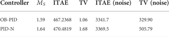
TABLE 1. Comparison of different controllers’ performance in Example 1.

FIGURE 2

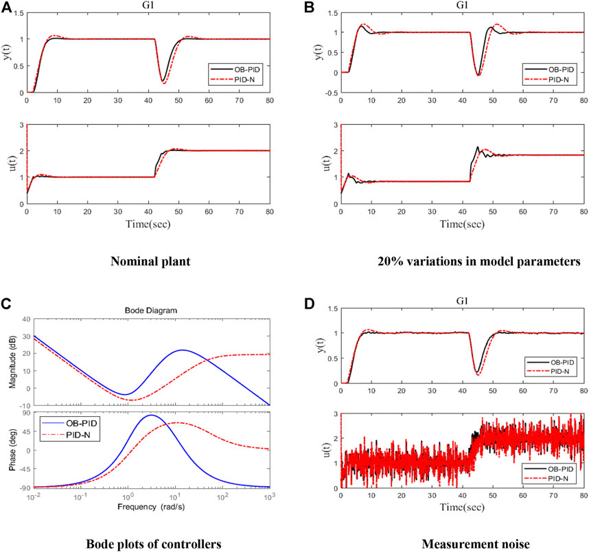
FIGURE 2. Responses for Example 1. (A) Nominal plant. (B) 20% variations in model parameters. (C) Bode plots of controllers. (D) Measurement noise.

Example 2. Considering the unstable process with a large time delay (USOPDT):

$\begin{array}{c}{\mathrm{G}}_2\left(s\right)=\frac{e^{-1.2s}}{\left(s-1\right)\left(0.5s+1\right)}\end{array}.(31)$

To tune a high-order PID for this plant, ${\omega }_c=0.37$ is chosen with the desired pole of the closed-loop placed at -2 to cancel $0.5s+1$; finally, we get a PIDD² with the following gains:

$\begin{array}{c}{K}_p=1.1625,K_i=0.0240,K_d=1.1808,K_{d2}=0.3028\end{array}.(32)$

The extended observer gain can be tuned with the observer bandwidth ${\overline{\omega }}_o=50$; thus, an observer-based PID with the following parameters can be obtained:

$\begin{array}{c}{\overline{K}}_o=\left[\begin{array}{cccc}0.3028& 1.1808& 1.1625& 0.0240\end{array}\right],b_0=1\end{array},$

$\begin{array}{c}{\overline{L}}_o={\left[\begin{array}{cccc}125000& 7500& 150& 1\end{array}\right]}^T,\alpha =0\end{array}.(33)$

Consider the controller designed by Shamsuzzoha and Lee (2009). A practical PID (n = 20) is implemented in practice for the controller:

$\begin{array}{c}{K}_{PID-N}=1.1165\left(1+\frac{1}{61.3412s}+\frac{0.4983s}{0.4983/Ns+1}\right)\left(\frac{0.6s+1}{0.0145s+1}\right)\end{array}.(34)$

The responses of the processes under the observer-based PID (33) proposed in this study and practical PID in Shamsuzzoha and Lee, (2009) are shown in Figure 3. Compared with the practical PID, the observer-based PID can achieve better tracking and disturbance rejection performance. The performance indexes for different controllers are listed in Table 2. It clearly shows that the observer-based PID (33) has better disturbance rejection performance and better control effort with smaller TV than the practical PID (34). Figure 3A shows the responses of closed-loop systems, where at t = 0 s, a unit step reference is inserted and a step disturbance input of magnitude 0.1 is inserted at t = 100 s. The red dotted dashed red line and black solid line represent the response of the practical PID form (34) and observer-based PID (33), respectively.It can be clearly seen from Figure 3A that the observer-based PID has better disturbance rejection and faster response speed than the practical PID in Shamsuzzoha and Lee, (2009). The Bode plots (Figure 3C) show that the observer-based PID (33) and the practical PID (34) roll off at high frequencies, thus attenuating measurement noise as expected. The observer-based PID has a larger roll-off rate; thus, the observer-based PID has better performance against high-frequency noise. In Figure 3D, the system with a white noise with a power of 0.00001, and a sampling period of 0.1 s is introduced into the process output. It shows that the proposed observer-based PID has better noise rejection performance than the practical PID (34). In the actual situation, there always exists a model mismatch. In order to evaluate the robustness of the controller, a 5% increase in the process gain and time delay and a 5% decrease in two-time constants are considered, i.e., the perturbed plant is ${\text{G}}_2^{\prime }\left(s\right)=1.05e^{-1.26s}/\left[\left(0.95s-1\right)\left(0.475s+1\right)\right]$. The responses are shown in Figure 3B. ITAE, robustness measure Ms, and TV of the control input u(t) for the system are also listed in Table 2. The TV of the observer-based PID is smaller and thus has better control effort. The simulation results show that the proposed observer-based PID gives better control performances both in the setpoint tracking and disturbance rejection performance than the practical PID as given in Shamsuzzoha and Lee, (2009).

FIGURE 3

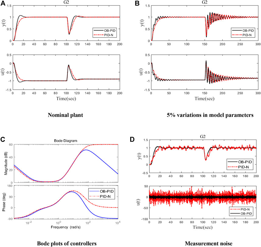
FIGURE 3. Responses for Example 2. (A) Nominal plant (b) 5% variations in model parameters. (C) Bode plots of controllers. (D) Measurement noise.

TABLE 2

TABLE 2. Comparison of different controllers’ performance in Example 2.

Example 3. The following second-order dead time process with two unstable poles process (SODPTUP) is considered:

$\begin{array}{c}{\mathrm{G}}_3\left(s\right)=\frac{2e^{-0.3s}}{\left(3s-1\right)\left(s-1\right)}\end{array}.(35)$

A two-degree-of-freedom control structure with a disturbance estimator in the form of the practical PID (n = 20) was proposed by Shamsuzzoha and Lee (2009) for this process:

$\begin{array}{c}{K}_{PID-N}=3.5671\left(1+\frac{1}{1.491s}+\frac{1.3364s}{1.3364/Ns+1}\right)\left(\frac{0.15s+1}{0.0058s+1}\right)\end{array}.(36)$

To tune a high-order PID for this plant, choose ${\overline{\omega }}_c=1.35$ and we get PIDD² with the following gains:

$\begin{array}{c}{K}_P=3.2194,K_i=1.7917;K_d=5.2097,K_{d2}=0.6010\end{array}.(37)$

The extended observer gain can be tuned with the observer bandwidth ${\overline{\omega }}_o=100$; thus, the observer-based PID with the following parameters can be obtained:

$\begin{array}{c}{\overline{K}}_o=\left[\begin{array}{cccc}0.6010& 5.2097& 3.2194& 7.1917\end{array}\right],b_0=1\end{array},$

$\begin{array}{c}{\overline{L}}_o={\left[\begin{array}{cccc}{100}^3& 3\times {100}^2& 300& 1\end{array}\right]}^T,\alpha =\text{0.2}.\end{array}(38)$

The performance indexes for different controllers are listed in Table 3. It clearly shows that the observer-based PID (38) has better robustness and control effort than the practical PID (36). Figure 4A shows the responses of the closed-loop system, where at t = 0 s, a unit step reference is inserted and a step disturbance input of magnitude 1 is inserted at t = 20 s. The red dotted dashed red line and black solid line represent the response of the practical PID form (36) and observer-based PID (38), respectively. The Bode plots (Figure 4C) show that the observer-based PID (38) and the practical PID (36) roll off at high frequencies, thus attenuating measurement noise as expected. The observer-based PID has a larger roll-off rate; thus, the observer-based PID has better performance against high-frequency noise. In Figure 4D, the system with a white noise with a power of 0.00001 and a sampling period of 0.1 s is introduced into the process output. In order to evaluate the robustness of the controller, a 20% increase in the process gain and time delay and a 20% decrease in two-time constant are considered, i.e., the perturbed plant is ${\mathrm{G}}_{\mathrm{3}}^{\prime }\left(s\right)=2.1e^{0.315s}/\left[\left(2.85s-1\right)\left(0.95s-1\right)\right]$. The responses are shown in Figure 4B. ITAE, robustness measure M_s, and TV of the control input u(t) for the system are also listed in Table 3. The two controllers have almost the same TV, thus having almost the same control effort when there is noise. The simulation results show that the proposed observer-based PID gives good control performances and good robustness and almost the same noise attenuation compared with the practical PID given in Shamsuzzoha and Lee, (2009).

TABLE 3

TABLE 3. Comparison of different controllers’ performance in Example 3.

FIGURE 4

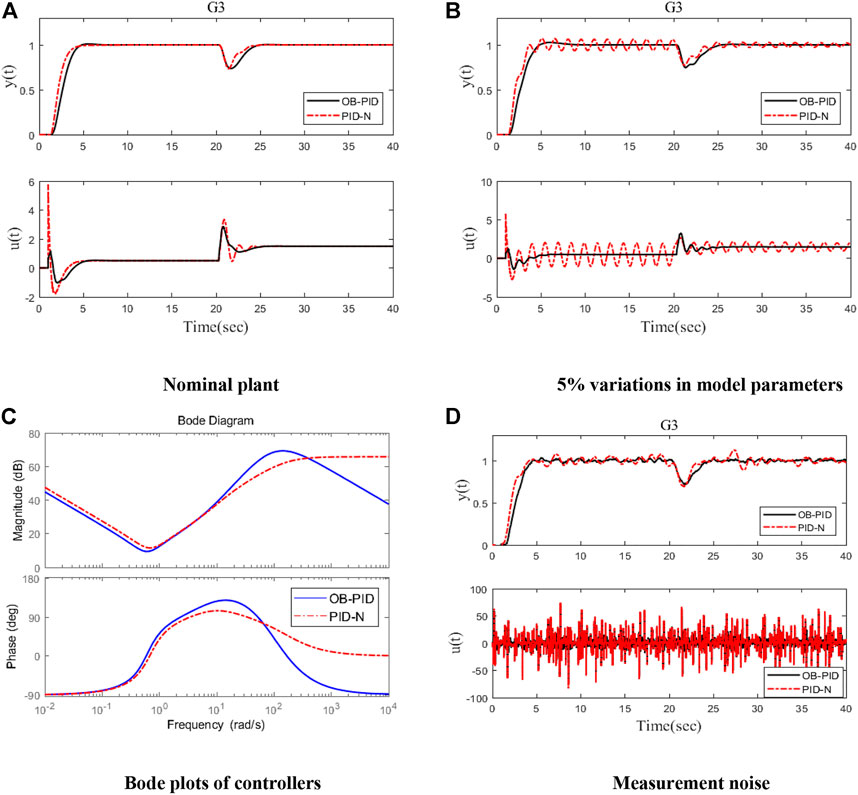
FIGURE 4. Responses for Example 3. (A) Nominal plant. (B) 5% variations in model parameters. (C) Bode plots of controllers. (D) Measurement noise.

Example 4. Considering the unstable process with an integrator:

$\begin{array}{c}{\mathrm{G}}_4\left(s\right)=\frac{{\mathrm{e}}^{-0.2}}{\mathrm{s}\left(s-1\right)}\end{array}.(39)$

To tune a high-order PID for this plant, choose ${\overline{\omega }}_c=1.5$ and we get a PIDD² with the following gains:

$\begin{array}{c}{K}_P=3.1320,K_i=1.7084,K_d=3.4771,K_{d2}=0.1564\end{array}.(40)$

With ${\overline{\omega }}_o=50$, we get a third-order observer-based PID with the following gains:

$\begin{array}{c}{\overline{K}}_o=\left[\begin{array}{cccc}0.1564& 3.4771& 3.1320& 1.7084\end{array}\right],b_0=1\end{array},$

$\begin{array}{c}{\overline{L}}_o={\left[\begin{array}{cccc}125000& 7500& 150& 1\end{array}\right]}^T,\alpha =0.1\end{array}.(41)$

For comparison, consider the two-degree-of-freedom control structure with a disturbance estimator in the form of the practical PID (n = 20) proposed by Shamsuzzoha and Lee, (2009) for this process.

$\begin{array}{c}{K}_{PID-N}=3.0241\left(1+\frac{1}{1.7941s}+\frac{1.058s}{1.058s/N+1}\right)\left(\frac{0.1s+1}{0.0087s+1}\right)\end{array}.(42)$

The performance indexes for different controllers are listed in Table 4. It clearly shows that the observer-based PID (41) has better control effort than the practical PID (42) but disturbance rejection performance and robustness similar to the practical PID. Figure 5A shows the responses of the closed-loop system, where at t = 0 s, a unit step reference is inserted and a step disturbance input of magnitude 1 is inserted at t = 15 s. The red dotted dashed red line and black solid line represent the response of the practical PID form (42) and observer-based PID (41), respectively.It can be clearly seen from Figure 5A that the observer-based PID has almost the same disturbance rejection performance as the practical PID as shown in Shamsuzzoha and Lee, (2009). The Bode plots (Figure 5C) show that the observer-based PID and the practical PID roll off at high frequencies, thus attenuating measurement noise as expected. The observer-based PID has a larger roll-off rate; thus, the observer-based PID has better performance against high-frequency noise. In Figure 5D, the system with a white noise with a power of 0.0001 and a sampling period of 0.1 s is introduced into the process output. It shows that the proposed observer-based PID has better noise rejection performance than the practical PID. In order to evaluate the robustness of the controller, a 10% increase in the process gain and time delay and a 10% decrease in the time constant are considered, i.e., the perturbed plant is ${\text{G}}_4^{\prime }\left(\mathrm{s}\right)=1.1{\mathrm{e}}^{-0.22\mathrm{s}}/\left[\mathrm{s}\left(0.9\mathrm{s}-1\right)\right]$. The responses are shown in Figure 5B. ITAE, robustness measure M_s, and TV of the control input u(t) for the system are also listed in Table 4. Simulation results show that the proposed observer-based PID has almost the same performance in disturbance rejection and robustness but better noise attenuation than the practical PID as shown inShamsuzzoha and Lee, (2009).

TABLE 4

TABLE 4. Comparison of different controllers’ performance in Example 4.

FIGURE 5

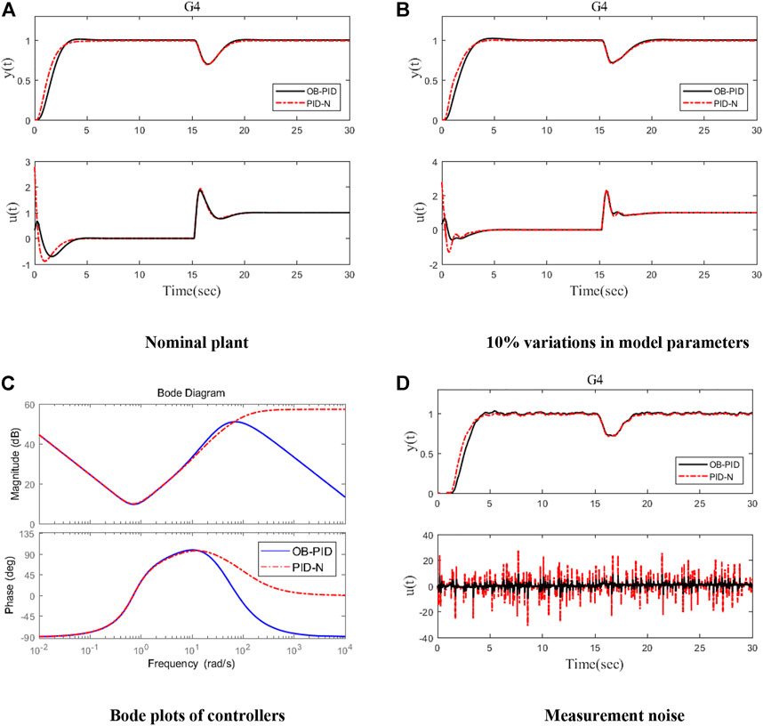
FIGURE 5. Responses for Example 4. (A) Nominal plant. (B) 10% variations in model parameters. (C) Bode plots of controllers. (D) Measurement noise.

5 Conclusion

A state feedback pole-placement method was proposed to design high-order PID controllers, and an observer-based PID structure was proposed to implement high-order PID controllers. The observer-based PID can effectively suppress noise by estimating the derivatives of the plant output through a model-independent observer. It was shown that the observer-based PID can be tuned with two parameters, ${\mathrm{\omega }}_{\mathrm{c}}$, for PID control gain, and ${\mathrm{\omega }}_{\mathrm{o}}$, for observer gain. Simulations for second-order processes with time delay showed that high-order PID may achieve better performance than the traditional PID, and the proposed observer-based PID can achieve a better tradeoff among disturbance rejection, robustness, and noise attenuation.

It is observed that if a cost function is used in the state-feedback design and observer design, then it can be directly related to an optimal controller; thus, an observer-based PID can also be designed via the well-known LQG method, which will be investigated in the future.

Data availability statement

The original contributions presented in the study are included in the article/Supplementary Material; further inquiries can be directed to the corresponding author.

Author contributions

WH substantially contributed to the conception and design of the work and the acquisition of data for the work. QH analyzed and interpreted data for the work. UD drew the picture and checked the work. WT revised the manuscript critically for important intellectual content.

Conflict of interest

The authors declare that the research was conducted in the absence of any commercial or financial relationships that could be construed as a potential conflict of interest.

Publisher’s note

All claims expressed in this article are solely those of the authors and do not necessarily represent those of their affiliated organizations, or those of the publisher, the editors, and the reviewers. Any product that may be evaluated in this article, or claim that may be made by its manufacturer, is not guaranteed or endorsed by the publisher.

References

Åström, K. J., and Hägglund, T. (2006). Advanced PID control. Research Triangle Park: ISA-The Instrumentation, Systems, and Automation Society 461.

Google Scholar

Åström, K. J., and Hägglund, T. (2001). The future of PID control. Control Eng. Pract. 9, 1163–1175. doi:10.1016/S0967-0661(01)00062-4

CrossRef Full Text | Google Scholar

Chen, D., and Seborg, D. E. (2002). PI/PID controller design based on direct synthesis and disturbance rejection. Ind. Eng. Chem. Res. 41, 4807–4822. doi:10.1021/ie010756m

CrossRef Full Text | Google Scholar

Dash, P., Saikia, L. C., and Sinha, N. (2015). Automatic generation control of multi area thermal system using Bat algorithm optimized PD–PID cascade controller. Int. J. Electr. Power & Energy Syst. 68, 364–372. doi:10.1016/j.ijepes.2014.12.063

CrossRef Full Text | Google Scholar

Du, Y., Cao, W., and She, J. (2022). Analysis and design of active disturbance rejection control with improved extended state observer for systems with measurement noise. IEEE Trans. Ind. Electron., 1. doi:10.1109/TIE.2022.3153821

CrossRef Full Text | Google Scholar

Duan, X. G., Li, H. X., and Deng, H. (2008). Effective tuning method for fuzzy PID with internal model control. Ind. Eng. Chem. Res. 47, 8317–8323. doi:10.1021/ie800485j

CrossRef Full Text | Google Scholar

Ediga, C. G., and Ambati, S. R. (2021). Measurement noise filter design for unstable time delay processes in closed loop control. Int. J. Dyn. Control 10, 138–161. doi:10.1007/s40435-021-00798-0

CrossRef Full Text | Google Scholar

Gao, Z. (2003). “Scaling and bandwidth-parameterization based controller tuning,” in Proceedings of the 2003 American Control Conference, 2003. Presented at the 2003 American Control Conference, Denver, CO, USA, 04-06 June 2003 (IEEE), 4989–4996. doi:10.1109/ACC.2003.1242516

CrossRef Full Text | Google Scholar

Garrido-Moctezuma, R., Suarez, D. A., and Lozano, R. (1997). “Adaptive LQG control of positive real systems,” in 1997 European Control Conference (ECC), Brussels, Belgium, 01-07 July 1997. doi:10.23919/ECC.1997.7082083

CrossRef Full Text | Google Scholar

Huba, M., Vrancic, D., and Bistak, P. (2021). PID control with higher order derivative degrees for IPDT plant models. IEEE Access 9, 2478–2495. doi:10.1109/ACCESS.2020.3047351

CrossRef Full Text | Google Scholar

Huba, M., and Vrani, D. (2018). “Comparing filtered PI, PID and PIDD 2 control for the FOTD plants,” in 3rd IFAC Conference on Advances in Proportional-Integral-Derivative Control, Ghent, Belgium, May 9–11, 2018 51 (4), 954–959.

CrossRef Full Text | Google Scholar

Latif, A., Shankar, K., and Nguyen, P. T. (2020). Legged fire fighter robot movement using PID. JRC. 1, 15–19. doi:10.18196/jrc.1104

CrossRef Full Text | Google Scholar

Lin, P., Wu, Z., Fei, Z., and Sun, X. M. (2021). A generalized PID interpretation for high-order LADRC and cascade LADRC for servo systems. IEEE Trans. Ind. Electron. 1, 5207–5214. doi:10.1109/tie.2021.3082058

CrossRef Full Text | Google Scholar

Mocci, J., Quintavalla, M., Chiuso, A., Bonora, S., and Muradore, R. (2020). PI-shaped LQG control design for adaptive optics systems. Control Eng. Pract. 102, 104528. doi:10.1016/j.conengprac.2020.104528

CrossRef Full Text | Google Scholar

Oliveira, V. A., Cossi, L. V., Teixeira, M., and Silva, A. (2009). Synthesis of PID controllers for a class of time delay systems. Automatica 45, 1778–1782. doi:10.1016/j.automatica.2009.03.018

CrossRef Full Text | Google Scholar

Sahib, M. A. (2015). A novel optimal PID plus second order derivative controller for AVR system. Eng. Sci. Technol. Int. J. 13, 194–206. doi:10.1016/j.jestch.2014.11.006

CrossRef Full Text | Google Scholar

Segovia, V. R., Hägglund, T., and Åström, K. J. (2014). Measurement noise filtering for PID controllers. J. Process Control 24, 299–313. doi:10.1016/j.jprocont.2014.01.017

CrossRef Full Text | Google Scholar

Shamsuzzoha, M., and Lee, M. (2009). Enhanced disturbance rejection for open-loop unstable process with time delay. ISA Trans. 48, 237–244. doi:10.1016/j.isatra.2008.10.010

PubMed Abstract | CrossRef Full Text | Google Scholar

Simanenkov, A. L., Rozhkov, S. A., and Borisova, V. A. (2017). “An algorithm of optimal settings for PIDD 2 D 3-controllers in ship power plant,” in 2017 IEEE 37th International Conference on Electronics and Nanotechnology (ELNANO) (IEEE), 152–155.

Google Scholar

Tan, W., Liu, J., Chen, T., and Marquez, H. J. (2006). Comparison of some well-known PID tuning formulas. Comput. Chem. Eng. 30, 1416–1423. doi:10.1016/j.compchemeng.2006.04.001

CrossRef Full Text | Google Scholar

Vrančić, D., and Huba, M. (2021). High-order filtered PID controller tuning based on magnitude optimum. Mathematics 9, 1340. doi:10.3390/math9121340

CrossRef Full Text | Google Scholar

Wang, Q., Lu, C., and Pan, W. (2016). IMC PID controller tuning for stable and unstable processes with time delay. Chem. Eng. Res. Des. 105, 120–129. doi:10.1016/j.cherd.2015.11.011

CrossRef Full Text | Google Scholar