Comparative analysis of different FOPI approximations and number of terms used on simulations of a battery-powered, field-oriented induction motor based electric vehicle traction system

Because of their enhanced performance, the fractional order proportional-integral (FOPI) controllers are becoming an appealing choice for controlling induction motor speed. To implement FOPI controllers, several fractional order integral approximations are available in the literature. The approximation used, and the order of approximation affects the speed tracking, transient response, and induction motor power consumption. This further affects the energy consumption analysis if simulations are conducted based on such approximations. In this paper an electric vehicle (EV) traction system is simulated to investigate the effect of such approximations on the simulations of a battery powered, induction motor driven EV system. The system consists of an indirect field-oriented induction motor, a lithium-ion battery bank, and a three-phase inverter. This work presents a quantitative analysis of the performance of FOPI controllers using different approximations, and order of approximations is presented. The controllers are evaluated based on speed tracking, transient response, computational time, and power consumption. Both step functions and standard drive cycles are used as the speed reference signal to evaluate the effects of using different approximations and different orders of approximation, when different references are used. This work establishes a reference set of simulations that can be used to infer the amount of error in battery state of charge, and state of health analysis conducted on such an EV system, when dealing with FOPI controllers under different approximations and related settings.

Introduction

Integer order PID controllers are a common choice for different control applications in the industry because of their simplicity of design and ease of implementation (Kalangadan, Priya and Kumar, 2015; George and Kamath, 2020). The performance of integer order PID controllers is impacted by the system non-linearities and uncertainty in parameters. The fractional order PI (FOPI) controllers allows to have fractional order integral in the control law. The order of the integral can be tuned which results in higher degree of flexibility. Thus, the FOPI controllers are more flexible as compared to integer order ones (HosseinNia et al., 2011). This added flexibility and tuning ability helps in achieving better dynamic response (Viola, Angel and Sebastian, 2017). Recently, the FOPI controllers have replaced traditional PID controllers for many speed control applications because of their better speed tracking performance and higher degree of flexibility (Dulau et al., 2017). The FOPI controllers have recently gained considerable attention in a variety of control applications. The fractional order controllers can help in achieving efficient control actions as the order of the fractional integral or derivative can be varied (Podlubny, 1999).

An intuitive explanation of fractional order PID (FOPID) controllers is given in (Tejado et al., 2019). Before going into FOPID controllers, first the classical PID controller is discussed. Classical PID controllers consist of three control actions, proportional, integral and derivative. The present (proportional action), the past (integral action) and predicted future (derivative action) error are all taken into account. The control law of a PID controller is given by:

$\begin{array}{c}u\left(t\right)=K_{p}e\left(t\right)+K_i{\displaystyle \underset{0}{\overset{t}{\int }}e\left(\tau \right)}d\tau +K_d\frac{de\left(t\right)}{dt}\end{array}(1)$

where e(t) is the error signal and u(t) is the control signal. The proportional component produces an output proportional to the current error; however, proportional action alone is not enough to eliminate steady state error. The integral term accumulates past error, and its main role is to guarantee the elimination of the steady state error. Lastly, the derivative action is a crude prediction of future error, the slope of the e(t) curve can be thought of as a linear extrapolation of the error at that point. The contributions of each control action are added, and the result is the control signal. FOPID controllers are the generalization of classical PID controllers to include non-integer order integrals and derivatives. The control law of an FOPID controller is given by:

$\begin{array}{c}u\left(t\right)=K_{p}e\left(t\right)+K_i{D}^{-\lambda }e\left(t\right)+K_d{D}^{\mu }e\left(t\right)\end{array}(2)$

where $\lambda$ and $\mu$ are the non-integer orders of the fractional integral and derivative terms respectively. $D$ is the fractional operator and is defined as follows:

$\begin{array}{c}{D}^{-n}f\left(t\right)=\frac{1}{\Gamma \left(n\right)}{\displaystyle \underset{0}{\overset{t}{\int }}f\left(\tau \right){\left(t-\tau \right)}^{n-1}}dy\end{array}(3)$

FOPID controllers are similar to PID controllers, in that they also take into account the past, present and future errors; however, due to the non-integer order, the integral and derivative actions are different than in the classical PID case.

The fractional integral term is no longer the typical area under the curve; however, it can be viewed as the area under a projection of the e(t) curve onto a plane which is determined by the order of integration. In doing so, the fractional integral action results in having a selective memory of the past error values.

The fractional derivative term can also be viewed as a prediction but does not use the slope and the tangent line passing through the point e(t), as in the case of the classical derivative action. The prediction in the fractional derivative case can be thought to be made through a non-tangent line passing through the point e(t), the slope of the line corresponds to the fractional differentiation with the order $\mu$ at that point. Another way of viewing the fractional derivative action is as if it is a non-linear extrapolation of the error as opposed to the linear extrapolation in the classical PID case. The non-linear extrapolation is based on the order of the fractional derivative.

The fractional order PI controllers can be estimated as a product of multiple poles and zeros. Thus, it can replace a lead-lag compensator with only three parameters to be tuned (Oustaloup et al., 2000). The FOPI controllers have been successfully applied for many practical applications including induction motor control, servo systems, hard disk drives and control of power electronic converters (Calderón et al., 2006; Luo et al., 2013; Tepljakov et al., 2016). The FOPI controllers have the ability to perform better as compared to the integer order PI controllers for the speed control of induction motors. The reason is that induction motor has a non-linear model (Upadhyaya and Gaur, 2021). The FOPI controllers are an extension of standard PI controllers introduced to improve the stability and robustness for the complex industrial and commercial systems with uncertain paraments (Upadhyaya and Gaur, 2021). In integer order PI controllers, the control signal is obtained by adding two terms. The first term is proportional to the error and the second term is proportional to the first order integral of error. The fractional order PI controllers also have control signal as sum of two terms. The first term is proportional to the error while the second term is proportional to the fractional order integral of the error (Duarte-Mermoud et al., 2010).

There are different approximations available for the fractional order integral term in the FOPI controller. The approximations considered in this paper are the Crone, Carlson and Matsuda approximations. The number of terms in the various approximations can also vary. The choice of different approximations and the number of terms can have an impact on the performance of FOPI controller for different applications. There is not much work available in the literature for the performance analysis and comparison of the different FOPI approximations. The goal of this work is to implement and compare the different available approximations of the FOPI controller on a simulation of an EV traction system. The EV model used in the simulations includes an induction motor powered by a lithium-ion battery bank. A simplified vehicle dynamics model is used for the estimation of the load torque on the induction motor (Chauhan, 2015). The simulations are carried out for different approximations of the FOPI controller using different number of terms. The EV model is simulated with different drive cycles and the performance of different FOPI approximations is analyzed. The metrics used for the comparison include speed error and the battery energy consumption. This work will help to determine which approximation of the FOPI controller is ideal for EV traction system control applications.

Fractional order integral approximations

FOPI controllers are more suited for non-linear systems where it can compensate for the variation of system parameters in addition for having better disturbance rejection (Usman et al., 2019). The main disadvantage of FOPI controllers is that they are more difficult to implement, and tune compared to linear PID controllers. However, many tools were created to ease this process at least in simulation such as the “Ninteger toolbox” (Valerio, 2005).

Different methods exist to approximate fractional order integrals and derivatives, three of which were tested, and their results analyzed in this work. The goal of a fractional order integral approximation is to provide a transfer function that is an approximation of the following transfer function shown below (Valerio, 2005):

$\begin{array}{c}C\left(s\right)=k{s}^v,v\in \mathrm{ℝ}\end{array}(4)$

Note that v here can be any real number and can take non-integer values. Three well known approximations are investigated in this work, the Crone, Carlson and Matsuda approximations. Note, the order of approximation is determined while designing the controllers (See the FOPI Controller Design Section for more details).

Crone approximation

The crone approximation is defined below (Oustaloup, 1991):

$\begin{array}{c}C\left(s\right)=k^{\prime }{\displaystyle \prod _{n=1}^N\frac{1+\frac{s}{{\omega }_{zn}}}{1+\frac{s}{{\omega }_{pn}}}}\end{array}(5)$

Where N is the order of the approximation and k′ is an adjustment gain used so that the gain of the resultant transfer function is 0 dB at a frequency of 1 rad/s. Here ${\text{ω}}_{zn}$ and ${\text{ω}}_{pn}$ are the zeros and poles of the transfer function. The poles and zeros of the transfer functions are calculated as shown below:

$\begin{array}{c}\alpha ={\left(\frac{{\text{ω}}_h}{{\text{ω}}_l}\right)}^{\frac{v}{N}}\end{array}(6)$

$\begin{array}{c}\eta ={\left(\frac{{\omega }_h}{{\omega }_l}\right)}^{\frac{1-v}{N}}\end{array}(7)$

$\begin{array}{c}{\text{ω}}_{z1}={\text{ω}}_l\sqrt{\text{η}}\end{array}(8)$

$\begin{array}{c}{\text{ω}}_{pn}={\text{ω}}_{z,n-1}\alpha , n=1,\dots ,N\end{array}(9)$

$\begin{array}{c}{\text{ω}}_{zn}={\text{ω}}_{p,n-1}\eta , n=2,\dots ,N\end{array}(10)$

The poles and zero frequencies are within ${\text{ω}}_h$ and ${\text{ω}}_l$, and the frequency range [${\text{ω}}_l$ , ${\text{ω}}_h$] is the frequency range for which the approximation is valid. The Crone approximation uses a recursive method to obtain the locations of the poles and zeros of the approximate transfer function, and the logarithms of the poles and zero frequencies will be equidistant. Note that if the value of v is negative then the roles of the poles and zeros are interchanged.

Carlson approximation

The Carlson approximation provides an approximation of a fractional order power of a transfer function using Newton’s iterative method (Carlson and Halijak, 1964). The power must be the inverse of an integer, as shown below:

$\begin{array}{c}C\left(s\right)=g^{\frac{1}{a}}\left(s\right)\end{array}(11)$

where g(s) in this case is taken to be s and with that an approximation for the following transfer function is obtained. The Carlson approximation is used to approximate a fractional order integral; however, the order of integration has to be the reciprocal of an integer “a.” If the order of integration cannot be expressed as a reciprocal of an integer, the nearest integer reciprocal is used, this is taken care of by the “Ninteger Toolbox” and “a” is chosen such that its reciprocal is the nearest to the desired order of approximation.

$\begin{array}{c}C\left(s\right)=s^{\frac{1}{a}}\end{array}(12)$

Note that here the fraction has to be the inverse of an integer and is rounded off to the nearest inverse of an integer. The following recursive expression is used to obtain the approximation, as shown below

$\begin{array}{c}{C}_n\left(s\right)=C_{n-1}\left(s\right)\frac{\left(a-1\right)C_{n-1}^a\left(s\right)+\left(a+1\right)g\left(s\right)}{\left(a+1\right)C_{n-1}^a\left(s\right)+\left(a-1\right)g\left(s\right)},n=1,\dots N\end{array}(13)$

where N is the order of the approximation, the Nth expression obtained from the recursive method above is a fractional integral approximation. This is an iterative process with the number of iterations being the order of the approximation. In the initial iteration the value of $C_0\left(s\right)$ is equal to 1.

Matsuda approximation

The Matsuda method is used to approximate a function f(x) whose value is known for a set of points $x_0,x_1,x_2,\dots ,x_N$. The following set of functions (d₀,…,d_N) are defined recursively as shown below (Matsuda and Fujii, 1993):

$\begin{array}{c}{d}_0\left(x\right)=f\left(x\right)\end{array}(14)$

$\begin{array}{c}{d}_{k+1}\left(x\right)=\frac{x-x_k}{d_k\left(x\right)-d_k\left(x_k\right)},k=\mathrm{0,1,2}\dots \end{array}(15)$

Using this set of functions, the function f(x) is approximated as shown below:

$\begin{array}{c}f\left(x\right)=d_0\left(x_0\right)+\frac{x-x_0}{d_1\left(x_1\right)+\frac{x-x_1}{d_2\left(x_2\right)+\frac{x-x_2}{d_3\left(x_3\right)+\frac{x-x_3}{\dots }}}}\end{array}(16)$

This method can be used to approximate the transfer function $C\left(s\right)=k{s}^v,v\in \mathrm{ℝ}$. To do so, first, the substitution $s=j\omega$ is made, as shown below;

$\begin{array}{c}C\left(\omega \right)=k{\left(j\omega \right)}^v,v\in \mathrm{ℝ}\end{array}(17)$

The value of the transfer function is computed at a set of N logarithmically evenly spaced frequencies. Where N is the order of the approximation.

$\begin{array}{c}{d}_0\left(\omega \right)=C\left(\omega \right)\end{array}(18)$

$\begin{array}{c}{d}_{k+1}\left(\omega \right)=\frac{\omega -{\omega }_k}{d_k\left(\omega \right)-d_k\left({\omega }_k\right)}\end{array}(19)$

$\begin{array}{c}C\left(\omega \right)=d_0\left({\omega }_0\right)+\frac{\text{s}-{\omega }_0}{d_1\left({\omega }_1\right)+\frac{\text{s}-{\omega }_1}{d_2\left({\omega }_2\right)+\frac{\text{s}-{\omega }_2}{d_3\left({\omega }_3\right)+\frac{\text{s}-{\omega }_3}{\dots }}}}\end{array}(20)$

For all three approximations, the parameters of the approximation are the frequency range, the order of the approximation and the fractional order of integration. The frequency range was chosen such that the frequency components of the input signals will be well within the frequency limits. There are three controllers based on the field-oriented control scheme used in this paper, an outer speed controller, an inner i_qs controller and an i_ds controller. For the case of the outer speed controller the fastest changing input is the NEDC drive cycle which provides the reference speed signal for the motor to track. This input speed reference is analyzed in frequency domain and it is found that the input speed reference is mainly comprised of low frequency components, with practically nothing beyond 1 Hz. The i_ds controller has a constant DC reference of 6A. For the inner i_qs controller, the frequency content of the reference i_qs corresponding to the NEDC drive cycle is analyzed. The frequency components of the reference i_qs signal also mainly consist of low frequency components with practically no components above 5 Hz or approximately 32 rad/sec. A safety margin was added and the frequency range was chosen to be between 0 and 100 rad/s which is more than a three times safety margin. This work focuses on the effect of the order of approximation and the approximation method on the speed tracking, transient response, and the energy consumption of a simulated EV traction system.

System modelling

This section discusses the theory and the modelling required to simulate an EV traction system using MATLAB. First, the theory behind the indirect field-oriented control scheme (used to control the speed of the induction motor) is given. Next, the vehicle dynamics modelling is discussed and how these dynamics translate into a load torque on the induction motor of the EV. Moreover, the modelling of a lithium-ion battery is discussed. Lastly, the overall Simulink block diagram of the EV traction system is given and discussed, along with the modelling parameters (induction motor parameters, vehicle model parameters and the battery model parameters)

Field oriented control of induction motors

Field Oriented Control (FOC) is a common motor control scheme used in high-performance drives. It offers better dynamic response and robustness in comparison with simpler scalar control schemes such as V/F, while at the same time adding more complexity to the system. However, advancements in the processing power of microcontrollers which can handle intensive mathematical operations made it possible for FOC to proliferate in the industry. The main principle of FOC is decoupling the torque and the magnetizing flux, thus allowing for direct control of the needed torque at any speed while maintaining the desired rotor flux. Decoupling is done through the control of stator currents, after transforming the three-phase time variant system into a two-phase time invariant system represented by d (the flux component) and q (the torque component) coordinates (Akin and Bhardwaj, 2019). Different types of controllers can be used to regulate the rotor flux, which is represented by i_sd, which makes torque control linearly related to the value of i_sq. One major requisite of FOC is aligning the rotor flux with the stator’s rotating synchronous reference frame. Different methods were developed to achieve this but we can group them into two categories: Indirect FOC (IFOC) and Direct FOC (DFOC). In DFOC, aligning of the rotor flux is implemented through direct sensing or estimating the flux in the air gap. This method might require the usage of physical sensors in the machine which makes it more difficult to implement both hardware and software wise, because the data gathered by the sensors needs to be processed and integrated in the control loop. One of the advantages of DFOC is that it is less affected by motor parameters variation and requires less knowledge about the parameters in general (Tripathi and Vaish, 2019). IFOC works without the need for sensing the actual flux, for it can be derived from the values of stator current, voltage and motor shaft speed (Tripathi and Vaish, 2019). In order to get accurate results for flux calculation, the controlled motor parameters must be fed to the control system. Which means that any variations in these values during different operation envelopes can degrade the performance of the drive system if not tuned with those cases in mind.

The work presented in this paper was implemented using an IFOC system. Two inner FOPI control loops regulate the values of i_sd and i_sq based on the reference values fed by the outer speed control loop in the case of i_sq, or a fixed step command reference for i_sd. The outer speed control loop is implemented using an FOPI controller. The electromagnetic torque produced by the induction motor and its mechanical model are given by:

$\begin{array}{c}{T}_e=\frac{3p{L}_m^2}{2L_r}{i}_{sd}{i}_{sq}\end{array}(21)$

$\begin{array}{c}J\frac{d{\omega }_r}{dt}=T_e-b{\omega }_r\end{array}(22)$

where L_m and L_r are the mutual inductance, J is the motor inertia, b is coefficient of viscous friction, p is the number of pole pairs and ω_r is the motor shaft speed. The overall block diagram of the IFOC of an induction motor is shown in Figure 1.

FIGURE 1

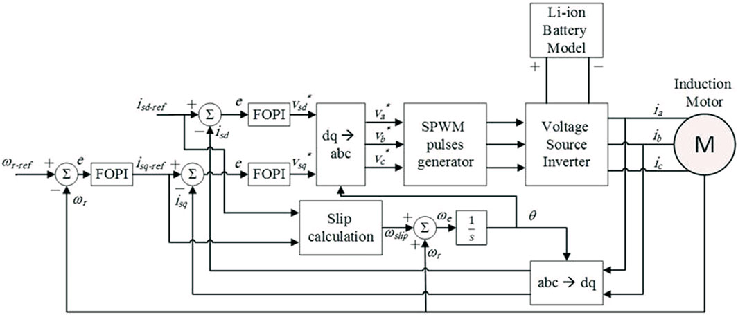
FIGURE 1. IFOC overall block diagram.

Vehicle modelling

The motor and the battery are the main components of the electric vehicle. The load torque can be defined as the rotational force required by the wheels to keep the vehicle moving. In an electric vehicle, the motor does not operate under no-load conditions. Load torque is applied to the motor depending on several factors, including weight, tire size, type of terrain, slope, and acceleration required (Chauhan, 2015).

Rolling resistance

The rolling resistance is the resistance between the vehicle rolling wheel and the road surface on which the vehicle is moving. The motor must overcome this resistance to keep the wheels of the vehicle rolling. The rolling resistance depends on the type of terrain and tires and is also proportional to vehicle weight. The higher the rolling resistance, the higher the power or torque required from the motor. The relation for the rolling resistance is given by:

$\begin{array}{c}Rolling Resistance \left(RR\right)=GVW \times C_{rr}\end{array}(23)$

where GVW is the gross weight of the vehicle and $C_{rr}$ is the rolling surface friction coefficient. The RR is the rolling friction on the wheels in Newtons.

Grade resistance

The slope of the surface plays an important role in the tractive force required by the electric vehicle. Gradient resistance is a form of gravitational force. The force applied to move the object up the inclined plane must overcome the vertical component of the weight. The mathematical relationship for grade resistance is given by:

$\begin{array}{c}Grade Resistance \left(GR\right)=GVWsin\left(\theta \right)\end{array}(24)$

where GR is the grade resistance to the uphill movement of the electric vehicle in Newtons. The angle $\theta$ is the slope of the terrain on which the car is moving on.

Acceleration force

The acceleration force required for the vehicle is equal to the product of the vehicle mass and the acceleration required. The acceleration that the electric vehicle can achieve is proportional to the torque of the motor. The acceleration force required for the vehicle is calculated using the following:

$\begin{array}{c}Acceleration Force \left(AF\right)=\frac{GVW}{g} a\end{array}(25)$

In the above equation, $g$ is the gravitational force and $a$ is the acceleration required by the vehicle. The AF is the corresponding acceleration force.

Air drag

Aerodynamic forces act as braking forces on the vehicle and tend to slow its motion. At low speeds, aerodynamic drag is negligible, but at high speeds it increases significantly. The mathematical relationship is given by:

$\begin{array}{c}Air Drag \left(AD\right)=0.5\rho CA{v}^2\end{array}(26)$

In the above equations, $\rho$ is the air density ($1.2754 kg/m^3$), $C$ is the vehicle air drag coefficient (typically 0.15), $A$ is the vehicle frontal area, and $v$ is the vehicle velocity.

Total tractive force

The total tractive effort (TTE) in newtons can be defined as the sum of all forces. The torque required by the vehicle is the product of the total tractive force and the radius of the wheels (Chauhan, 2015) as seen below:

$\begin{array}{c}Total Tractive Effort \left(TTE\right)=RR+GR+AF+AD\end{array}(27)$

$\begin{array}{c}Load Torque \left(T_c\right)=TTE \times R_{wheel} \end{array}(28)$

where R_wheel is the radius of the wheels of the vehicle.

Battery modelling

In order to simulate a real-life EV traction system, an equivalent circuit model (ECM) of a lithium-ion battery (Chen and Rincon-Mora, 2006) is used. The model takes the load current as an input and captures the voltage transients of a lithium-ion battery (Chen and Rincon-Mora, 2006). Figure 2 shows the ECM used to model the lithium-ion battery used in this work.

FIGURE 2

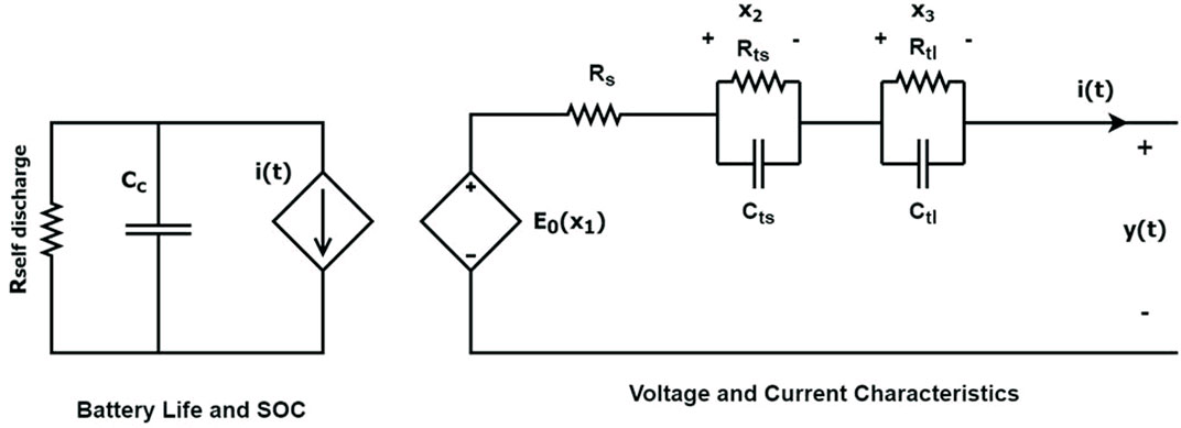
FIGURE 2. Battery Equivalent Circuit Model (ECM).

The left side of the ECM captures the state of charge of the battery as well as the self-discharge of the battery. The self-discharge resistance is ignored and is accounted for by multiplying the SOC by a factor f, which in this work is taken to be 1. The right side of the ECM captures the voltage characteristics of the lithium-ion battery. The voltage source (E₀) represents the open circuit voltage of the battery, R_s captures the battery series resistance, the R_ts||C_ts RC branch captures the short-term terminal voltage transient and the R_tl||C_tl RC branch captures the long-term terminal voltage transient of the battery. The state space equations of the ECM are shown below:

$\begin{array}{c}{\dot{x}}_1\left(t\right)=-\frac{1}{C_c}i\left(t\right)\end{array}(29)$

$\begin{array}{c}{\dot{x}}_2\left(t\right)=-\frac{x_2\left(t\right)}{R_{ts}\left(x_1\right)C_{ts}\left(x_1\right)}+\frac{i\left(t\right)}{C_{ts}\left(x_1\right)}\end{array}(30)$

$\begin{array}{c}{\dot{x}}_3\left(t\right)=-\frac{x_3\left(t\right)}{R_{tl}\left(x_1\right)C_{tl}\left(x_1\right)}+\frac{i\left(t\right)}{C_{tl}\left(x_1\right)}\end{array}(31)$

$\begin{array}{c}y=E_0\left(x_1\right)-x_2\left(t\right)-x_3\left(t\right)-i\left(t\right)R_s\left(x_1\right)\end{array}(32)$

where C_c is the battery capacity. Moreover, the circuit parameters (R_ts, C_ts, R_tl, C_tl, R_s, E₀) are all functions of the battery SOC given as follows:

$\begin{array}{c}{R}_{ts}\left(x_1\right)=a_1{e}^{-a_2{x}_1}+a_3\end{array}(33)$

$\begin{array}{c}{R}_{tl}\left(x_1\right)=a_4{e}^{-a_5{x}_1}+a_6\end{array}(34)$

$\begin{array}{c}{C}_{ts}\left(x_1\right)=-a_7{e}^{-a_8{x}_1}+a_9\end{array}(35)$

$\begin{array}{c}{C}_{tl}\left(x_1\right)=-a_{10}{e}^{-a_{11}{x}_1}+a_{12}\end{array}(36)$

$\begin{array}{c}{R}_s\left(x_1\right)=a_{13}{e}^{-a_{14}{x}_1}+a_{15}\end{array}(37)$

$\begin{array}{c}{E}_0\left(x_1\right)=-a_{16}{e}^{-a_{17}{x}_1}+a_{18}+a_{19}{x}_1-a_{20}{x}_1^2+a_{21}{x}_1^3\end{array}(38)$

where a₁, a₂, … , a₂₁ are positive constants. By knowing the values of these constants, the electrical characteristics and output voltage of a lithium-ion battery can be modeled. The output voltage of the battery model is used as an input to a controlled DC source block in Simulink which simulates a voltage equal to that of the input. Furthermore, the resulting DC current is measured and is fed back to the battery model in order to capture the battery voltage transients.

Overall system

After implementing the individual parts of the simulations discussed above using MATLAB and Simulink, the individual components were combined to obtain a simulated EV traction system. This EV system employs an IFOC scheme to control an induction motor which drives the vehicle. Furthermore, the EV system captures both the vehicle and the battery dynamics. The overall Simulink block diagram is shown in Figure 3.

FIGURE 3

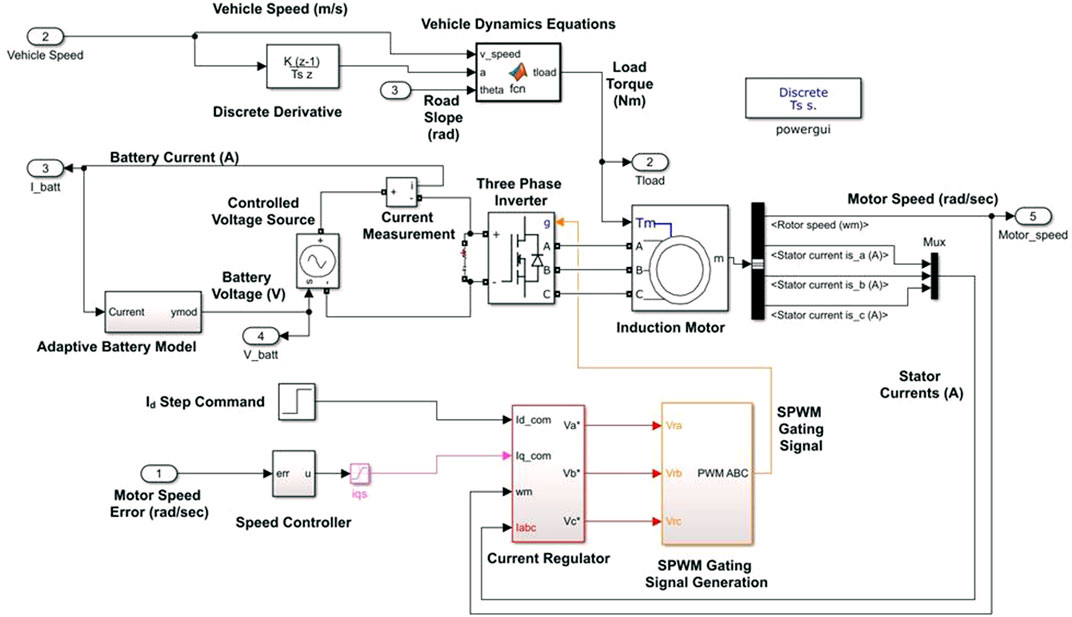
FIGURE 3. Simulink block diagram of the overall EV traction system.

At the bottom of Figure 3 the motor speed error is input to the outer FOPI speed controller. The outer controller produces the i_qs reference signal which along with the constant i_ds reference is fed into the current regulator. The current regulator block contains 2 FOPI controllers as shown in Figure 1. In the IFOC control scheme. From the two current controllers the v_sd^∗ and the v_sq^∗ signals are obtained, which are then converted from the d-q axis values to abc 3 phase voltages. The 3 phase voltage signals are used along with a triangular waveform to implement sinusoidal pulse width modulation from which the inverter gating signals are obtained. The 3-phase inverter powers the induction motor, it is controlled using the gating signals produced from the IFOC control scheme and is powered by a controlled DC voltage source. The voltage of this voltage source is set to be equal to the output voltage of the battery model. The battery model takes the current drawn as an input and gives the corresponding voltage output. Lastly, we have the vehicle dynamics equations implemented in the MATLAB function block seen at the top of Figure 3. The function block takes the vehicle speed, vehicle acceleration and road slope angle as inputs and uses the vehicle dynamics equations to obtain the corresponding load torque on the induction motor. The vehicle and induction motor parameters used in the simulation are summarized in Table 1. Also, the battery model parameters obtained from (Ali, Mukhopadhyay and Rehman, 2016) are also given in Table 1.

TABLE 1

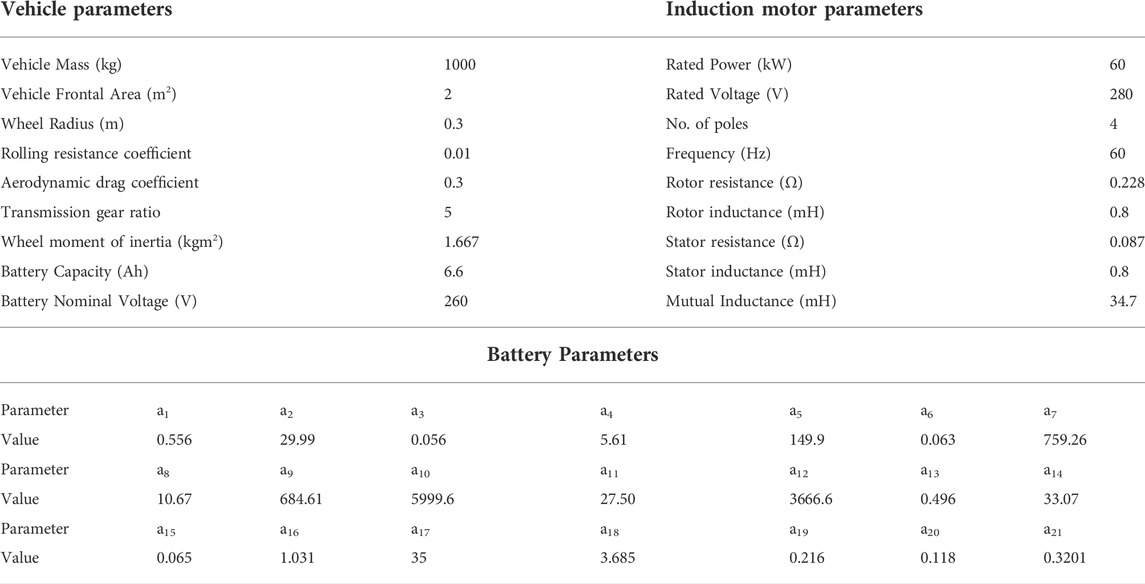
TABLE 1. Vehicle and induction motor parameters.

A transmission gear ratio of 5 was determined to be ideal for the given induction motor, as it will allow the motor to reach speeds close to the rated speed of the motor for a vehicle speed within 40 km/h. The vehicle speed is calculated from the motor speed, assuming the wheels do not slide on the surface, as shown below:

$\begin{array}{c}v=\frac{\omega r}{G}\end{array}(39)$

where v is the vehicle speed (m/s), $\text{ω}$ is the motor speed (rad/sec), r is the radius of the wheel (m) and G is the transmission gear ratio.

FOPI controller design

As mentioned in the System Modelling Section there are two cascaded FOPI controllers in the IFOC scheme. The outer controller is for the speed of the motor and the inner controller controls the i_sq current which in turn controls the motor torque. Furthermore, there is another controller to control the i_sd current which in turn controls the magnetic flux of the motor. To design these FOPI controllers a transient response-based method along with appropriate tuning rules are used to obtain the gains of each controller (Chen et al., 2008). These rules are based on maximum sensitivity constrained integral gain optimization (MIGO) tuning method; however, the tuning rules were generalized to encompass fractional order PI controllers. The rules were developed by maximizing the integral gain (K_i) while imposing constraints on the maximum output sensitivity and the resonance peak of the closed loop system. The tuning method involves first obtaining a step response of the plant that the controller will control. An appropriate step input is given to the plant, in case of the i_sq and i_sd controllers a v_sd and v_sq step is given respectively. Additionally, in the case of the outer speed controller an i_sq-ref step is given. Using these responses an approximate first order plus dead time (FPDT) model is fitted to the responses. The transfer function of an FPDT model is shown below:

$\begin{array}{c}{G}_{approx}\left(s\right)=\frac{K_{prcs}}{Ts+1}{e}^{-Ls}\end{array}(40)$

where $K_{prcs}$ is the process gain, $T$ is the time constant and $L$ is the dead time of the FPDT model. After obtaining the transient response corresponding to the i_sd controller the MATLAB PID tuner toolbox was used to fit an FPDT model to the response and obtain the values of K_prcs, T and L. The next step would be to use these parameter values along with the tuning rules shown in (41–45) to obtain the values of the proportional gain (K_p), integral gain (K_i), and the fractional order of the integral (α). The order of the fractional integral depends on the relative dead time $\tau$, as shown below. The authors in (Chen et al., 2008) conducted several tests on a variety of systems with varying values of $\tau$ and system delay L, from which the tuning rules were determined.

$\begin{array}{c}\tau =\frac{L}{T+L},\alpha =\left\{\begin{array}{cc}1.1,& \tau \ge 0.6\\ \begin{array}{c}1,\\ 0.9,\end{array}& \begin{array}{c}0.4\le \tau <0.6\\ 0.1\le \tau <0.4\end{array}\\ 0.7,& \tau <0.1\end{array}\right\}\end{array}(41)$

$\begin{array}{c}{K}_p=\frac{1}{K_{prcs}}\left(\frac{0.2978}{L+0.000307}\right)\end{array}(42)$

$\begin{array}{c}{T}_i=T\left(\frac{0.8578}{L^2-3.402L+2.405}\right)\end{array}(43)$

$\begin{array}{c}{K}_i=\frac{K_p}{T_i}\end{array}(44)$

The same process is then repeated for the i_sq controller and then the outer speed controller as well. The transient responses used to tune the individual controllers along with the fitted FPDT model responses are shown in Figure 4.

FIGURE 4

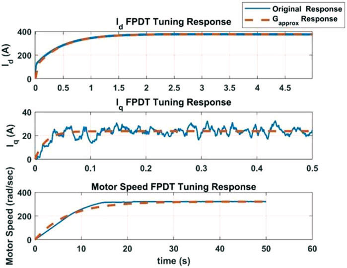
FIGURE 4. FPDT tuning responses.

As seen from Figure 4, the original responses (i.e., the step responses that were measured to obtain the FPDT model of the plant for each of the three controllers) and the step response of the resulting FPDT models do match up, supporting the claim that the FPDT model is an approximate model of the plant. Table 2 summarizes the FPDT parameter values for each of the three controllers along with the calculated gains (K_p and K_i) and order of integration ($\text{α}$).

TABLE 2

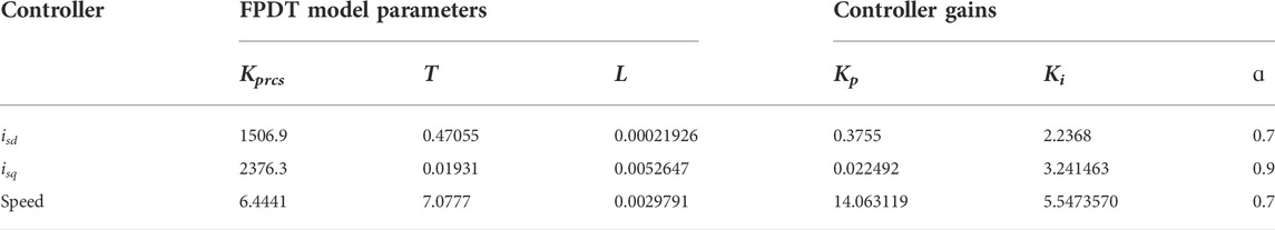
TABLE 2. FPDT parameter values and controller gains.

Results and discussion

The goal of this work is to thoroughly test the three FOPI approximations (Carlson, Crone and Matsuda) and compare them in terms of their speed tracking, power consumption and transient response. Furthermore, the effect of the order of approximation on the above-mentioned metrics is also analyzed for each of the three approximations at hand. A 35 km/h step input was given as an input reference to the system and the transient speed response was collected and analyzed for various order of approximations ranging between 4 and 14. This is to see the effect the order of approximation has on the transient response (settling time, % overshoot) and to also compare the three approximations against each other. The same was also done with a 22.6 km/h square wave and a 11.3 km/h square wave speed reference. Secondly, the NEDC drive cycle was used as an input speed reference to the system, this is to mimic real driving conditions which is more realistic than step responses. The NEDC drive cycle represents the typical European vehicle usage in urban and extra-urban (high speed situations) conditions and was used as the speed reference. The same input reference was applied for all the three approximations, each for various values of the order of approximation. The mean absolute speed error, the mean absolute power consumption, and the remaining SOC in the battery at the end of the drive cycle were obtained.

Step response and square wave tests

As mentioned, a 35 km/h step reference, along with a 11.3 km/h square wave (Square Wave 1) and a 22.5 km/h square wave (Square Wave 2) speed reference were applied to the system for all the three approximations and for a variety of order of approximations. The i_sd, i_sq, vehicle speed, battery current, battery voltage and battery consumed power are plotted in Figures 5–7. Figures 5–7 show the i_sd, i_sq, vehicle speed, battery current, battery voltage and battery consumed power for only one case. The same procedure was repeated for all three approximations for order of approximations ranging between 4 and 14. The settling time and maximum overshoot was noted in each case and is depicted in Figure 8.

FIGURE 5

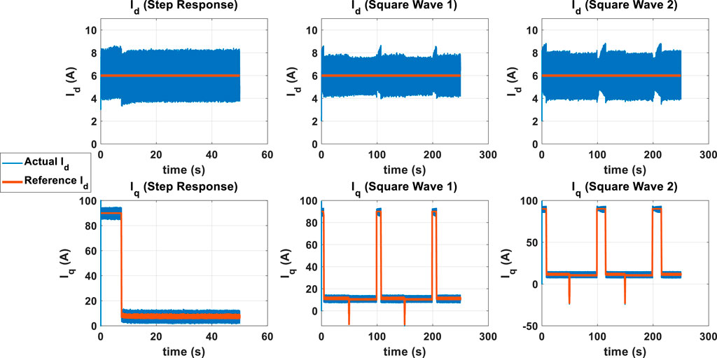
FIGURE 5. I_d and I_q response for step and square wave inputs.

FIGURE 6

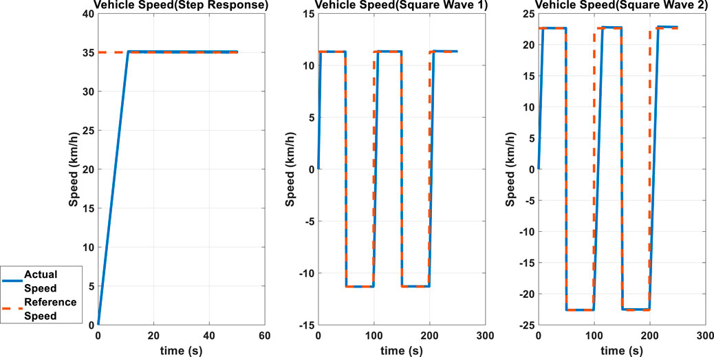
FIGURE 6. Vehicle speed response for step and square wave inputs.

FIGURE 7

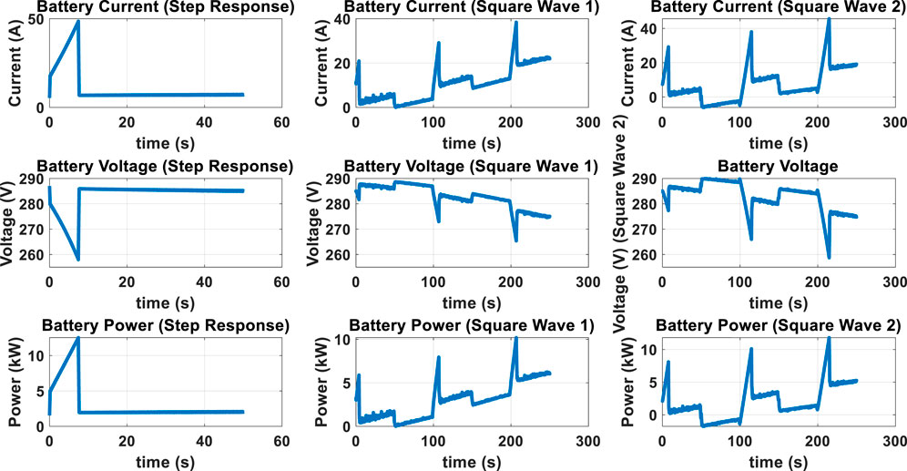
FIGURE 7. Battery current, voltage and power for step input.

FIGURE 8

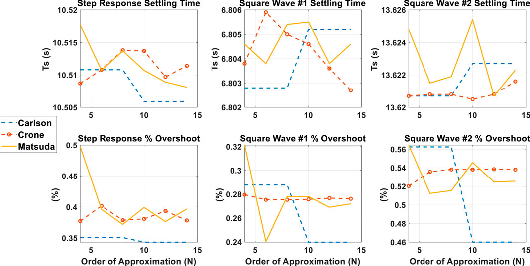
FIGURE 8. Settling time and overshoot of speed step response.

It can be observed from Figure 8 that for low orders of approximation the Matsuda approximation yields a large overshoot which decreases sharply with the lowest overshoot being around an order of approximation of 6 or 8. The Carlson approximation does result in higher overshoot at lower orders of approximation, and this is more evident in the square wave cases than the step response case. Furthermore, at low orders of approximation the Carlson approximation yields a lower settling time in both the square wave and in the step input cases.

Drive cycle tests

The second set of tests done were using the NEDC drive cycle as an input speed reference, to emulate vehicle speed during realistic driving conditions. The i_sd, i_sq, vehicle speed, battery current, battery voltage and battery consumed power for the drive cycle tests are shown in Figures 9–11.

FIGURE 9

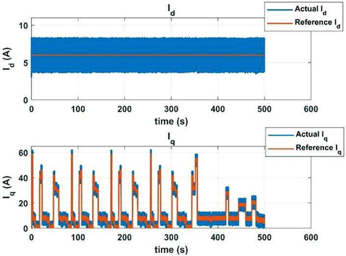
FIGURE 9. Id and iq response for a NEDC drive cycle input.

FIGURE 10

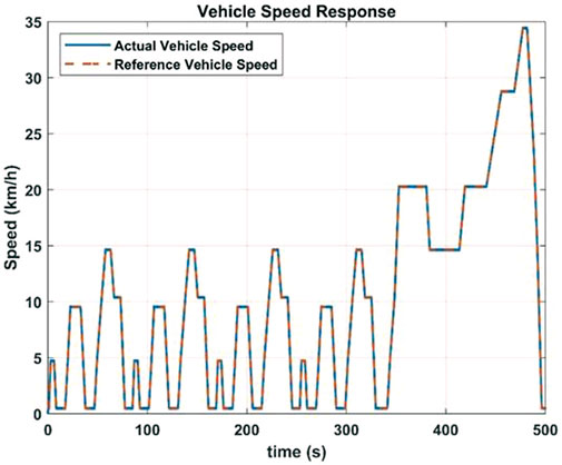
FIGURE 10. Vehicle speed response for NEDC drive cycle input.

FIGURE 11

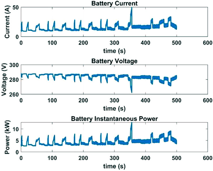
FIGURE 11. Battery current, voltage and power for NEDC drive cycle input.

Figures 9–11 show the i_sd, i_sq, vehicle speed, battery current, battery voltage and battery consumed power for only one case. The same procedure was repeated for all three approximations for order of approximations ranging between 4 and 14. For each case, the mean absolute speed error and mean absolute power consumed from the battery were obtained and are shown in Figure 12.

FIGURE 12

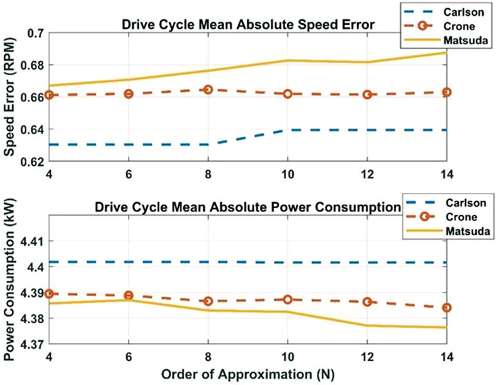
FIGURE 12. Mean absolute speed error and power consumption.

It can be observed from Figure 12 that the Carlson approximation results in the lowest mean absolute speed error, indicating better speed tracking performance. However, the enhanced speed tracking comes at the price of larger power consumption. The Carlson approximation results in roughly a 5% lower speed tracking error at low orders of approximation when compared to Crone or Matsuda but, on the other hand, consumes roughly 0.3% more power than the other two approximations. At higher orders of approximation (12–14), the Crone approximation performance in terms of speed error improves whereas it worsens the case of Carlson and Matsuda. Nevertheless, the Carlson approximation still results in 3.5% less speed tracking error when compared to Crone and almost 7% less speed tracking error when compared to Matsuda. Additionally, as the order of approximation increases, it can be observed that the power consumption for the Crone and Matsuda approximations reduces while there is little to no change in the case of the Carlson approximation. Also, the Carslon approximation at high orders of approximation (12–14) consumes 0.4% more power compared to Crone and 0.6% more than Matsuda.

The battery SOC at the end of the drive cycle tests is shown in the left column for each approximation in the top section in Table 3. Since, the same drive cycle was used, the same distance will be covered at the end of the tests regardless of the approximation. Therefore, for comparison purposes, the distance covered while consuming quarter of the battery capacity (i.e. starting from 100% SOC and ending at 75% SOC) was noted and is given in the right column for each approximation in the top section of Table 3. The results shown in Table 3 solidify the findings that the Matsuda approximation results in the least power consumption of the three approximations. This can be observed by the larger distance covered and the larger remaining SOC in the battery at the end of the drive cycle test. Furthermore, Table 3 also shows an increase in distance covered and increase in remaining SOC as the order of approximation increases, indicating that power consumption decreases as order of approximation increases for the Crone and Matsuda approximations; however, this is not the case for the Carlson approximation. This indicates the order of approximation has a smaller effect on the power consumption in the case of the Carlson rather than the Crone and Matsuda approximations.

TABLE 3

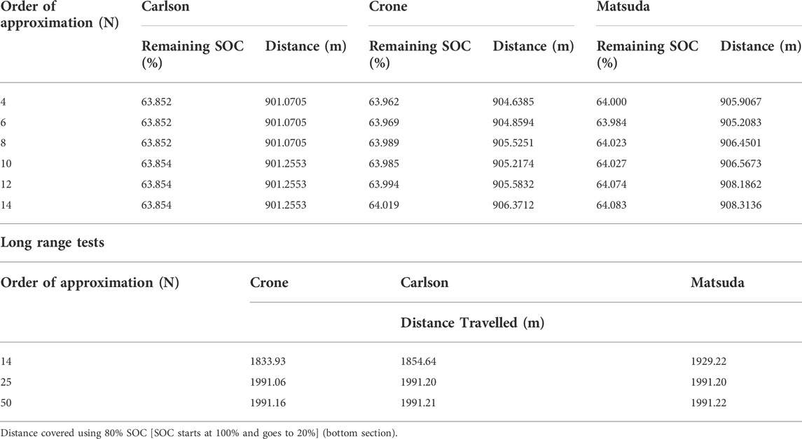
TABLE 3. Remaining SOC at the end of drive cycle and distance covered using 25% SOC [SOC starts at 100% and goes to 75%] (top section).

To further show the effect of the choice of approximation and order of approximation has on the energy consumption, another test was conducted. The simulation was kept running through multiple iterations of the NEDC drive cycle as an input speed reference. The simulation was kept running with the battery SOC initially set to 100% until the battery SOC reached 20%.

It is clear from the results given in the top section of Table 3, that the Crone approximation with an order of approximation of four produces the least driving range and consumes more battery charge for the same distance. The additional long-range tests will compare the most energy efficient case for all three approximations (order of approximation 14) with the overall worst case which is using the Crone approximation with an order of approximation of 4. Additionally, the tests were repeated for higher orders of approximation such as N = 25 and N = 50. The simulation was kept running until the stopping criteria (20% battery SOC) was reached and the distance covered in each case was noted.

In the least energy efficient case (Crone, N = 4), the vehicle was able to cover a distance of 1812.16 m. The vehicle was able to cover 1833.9, 1854.6 and 1929.2 m for the Crone, Carlson and Matsuda cases respectively with N = 14. However, at larger orders of approximation (N = 25 or N = 50) the distance covered using the three approximations become very similar with all of them covering roughly 1991.2 m, these results are summarized in the bottom section of Table 3. This shows that the choice of approximation and order of approximation has a greater effect on the vehicle range at lower orders of approximations. Although the computation time and effort are greatly increased as the order of approximation increases.

At lower orders of approximation (up to N = 14), the choice of approximation and order of approximation can lead to discrepancies in the distance covered by up to 117 m in one charge cycle of the battery (between the Crone approximation with N = 4 and the Matsuda approximation with N = 14), assuming the maximum depth of discharge of the battery of 80%. This is a 6% difference in the driving range and over multiple charge cycle this will add up. The results indicate that using the Matsuda approximation will lead to more energy saving in the long run. Also, this will lead to less number of charge cycles for the battery prolonging the battery life.

A trend of improved power consumption is observed as the order of approximation increases, with the performance (in terms of power consumption) being almost the same across all approximations at larger order of approximation (N = 25 or N = 50). However, the Matsuda approximation resulted in a larger improvement in the power consumption at lower orders of approximation, i.e., imposing lower computation cost and computational time requirements. Similar power consumption can be achieved by the other approximations; however, at larger order of approximation resulting in larger computational time and effort. Therefore, the Matsuda approximation may be preferred in applications where lower computational time and effort is preferred as it resulted in the least power consumption at lower order of approximation (up to N = 14).

Conclusion

If fractional order speed controllers are used for controlling the motor speed of an EV, the results indicate that the order of approximation and method of approximation used has definite effects on estimating the driving range of an EV. This has the potential to accumulate over time resulting in large effects on overall energy consumption and reduced driving range compared to what is expected. It is also seen from the results that there is a tradeoff between power consumption and speed tracking performance. Compromising on the motor speed tracking performance has the ability to reduce power consumption and improve driving range when a particular fractional order controller is used with a fixed and not very high order of approximation.

Data availability statement

The original contributions presented in the study are included in the article, further inquiries can be directed to the corresponding author.

Author contributions

SM and HR contributed to the conception and design of the study. MuE implemented the vehicle dynamics model and the Li-ion battery model. MaE and FA worked on the implementation of the IFOC scheme for an induction motor in Simulink. MaE worked on the tuning of the FOPI controllers. MaE and FA collected all the data needed for the comparative analysis. MaE, MuE, and FA all contributed to writing the manuscript. All authors were involved in the revision and approval of the final manuscript.

Funding

This work was supported in part by the faculty research grants FRG20-M-E95, FRG22-C-E09, and FRG22-C-E33.

Conflict of interest

The authors declare that the research was conducted in the absence of any commercial or financial relationships that could be construed as a potential conflict of interest.

Publisher’s note

All claims expressed in this article are solely those of the authors and do not necessarily represent those of their affiliated organizations, or those of the publisher, the editors and the reviewers. Any product that may be evaluated in this article, or claim that may be made by its manufacturer, is not guaranteed or endorsed by the publisher.

References

Akin, B., and Bhardwaj, M. (2019). Sensored field oriented control of 3-phase induction motors. Texas Instrument Guide. Report.

Google Scholar

Ali, D., Mukhopadhyay, S., and Rehman, H. (2016). “A novel adaptive technique for Li-ion battery model parameters estimation,” in 2016 IEEE National Aerospace and Electronics Conference (NAECON) and Ohio Innovation Summit (OIS), Ohio, USA, 25-29 July 2016 (IEEE), 23–26.

CrossRef Full Text | Google Scholar

Calderón, A. J., Vinagre, B. M., and Feliu, V. (2006). Fractional order control strategies for power electronic buck converters. Signal Process. 86 (10), 2803–2819. doi:10.1016/j.sigpro.2006.02.022

CrossRef Full Text | Google Scholar

Carlson, G., and Halijak, C. (1964). Approximation of fractional capacitors (1/s)^(1/n) by a regular Newton process. IEEE Trans. Circuit Theory 11 (2), 210–213. doi:10.1109/tct.1964.1082270

CrossRef Full Text | Google Scholar

Chauhan, S. (2015). Motor torque calculations for electric vehicle. Int. J. Sci. Technol. Res. 4 (8), 126–127.

Google Scholar

Chen, M., and Rincon-Mora, G. A. (2006). Accurate electrical battery model capable of predicting runtime and IV performance. IEEE Trans. Energy Convers. 21 (2), 504–511. doi:10.1109/tec.2006.874229

CrossRef Full Text | Google Scholar

Chen, Y., Bhaskaran, T., and Xue, D. (2008). Practical tuning rule development for fractional order proportional and integral controllers. J. Comput. Nonlinear Dyn. 3 (2). doi:10.1115/1.2833934

CrossRef Full Text | Google Scholar

Duarte-Mermoud, M. A., Mira, F. J., Pelissier, I. S., and Travieso-Torres, J. C. (2010). Evaluation of a fractional order PI controller applied to induction motor speed control. IEEE ICCA 2010, 573–577.

CrossRef Full Text | Google Scholar

Dulău, M., Gligor, A., and Dulău, T. M. (2017). Fractional order controllers versus integer order controllers. Procedia Eng. 181, 538–545. doi:10.1016/j.proeng.2017.02.431

CrossRef Full Text | Google Scholar

George, M. A., and Kamath, D. V. (2020). “Design and tuning of fractional order pid (FOPID) controller for speed control of electric vehicle on concrete roads,” in 2020 IEEE International Conference on Power Electronics, Smart Grid and Renewable Energy (PESGRE2020), Kerala, India, 2-4 Jan. 2020, 1–6.

CrossRef Full Text | Google Scholar

HosseinNia, S. H., Tejado, I., Vinagre, B. M., Milanés, V., and Villagrá, J. (2011). “Low speed control of an autonomous vehicle using a hybrid fractional order controller,” in The 2nd International Conference on Control, Instrumentation and Automation, Shiraz, Iran, 27-29 Dec. 2011, 116–121.

CrossRef Full Text | Google Scholar

Kalangadan, A., Priya, N., and Kumar, T. S. (2015). “PI, PID controller design for interval systems using frequency response model matching technique,” in 2015 International Conference on Control Communication & Computing India (ICCC), Kerala, India, 19-21 Nov, 119–124.

CrossRef Full Text | Google Scholar

Luo, Y., Zhang, T., Lee, B., Kang, C., and Chen, Y. (2013). Fractional-order proportional derivative controller synthesis and implementation for hard-disk-drive servo system. IEEE Trans. Control Syst. Technol. 22 (1), 281–289. doi:10.1109/tcst.2013.2239111

CrossRef Full Text | Google Scholar

Matsuda, K., and Fujii, H. (1993). H (infinity) optimized wave-absorbing control-Analytical and experimental results. J. Guid. Control, Dyn. 16 (6), 1146–1153. doi:10.2514/3.21139

CrossRef Full Text | Google Scholar

Oustaloup, A. (1991). La commande crone : commande robuste d'ordre non entier. Paris: Hermès (Traité des nouvelles technologies. Série automatique).

Google Scholar

Oustaloup, A., Levron, F., Mathieu, B., and Nanot, F. M. (2000). Frequency-band complex noninteger differentiator: characterization and synthesis. IEEE Trans. Circuits Syst. I. 47 (1), 25–39. doi:10.1109/81.817385

CrossRef Full Text | Google Scholar

Podlubny, I. (1999). Fractional-order systems and PI/sup/spl lambda//D/sup/spl mu//-controllers. IEEE Trans. Autom. Contr. 44 (1), 208–214. doi:10.1109/9.739144

CrossRef Full Text | Google Scholar

Tepljakov, A., Gonzalez, E. A., Petlenkov, E., Belikov, J., Monje, C. A., and Petráš, I. (2016). Incorporation of fractional-order dynamics into an existing PI/PID DC motor control loop. ISA Trans. 60, 262–273. doi:10.1016/j.isatra.2015.11.012

PubMed Abstract | CrossRef Full Text | Google Scholar

Tripathi, S. M., and Vaish, R. (2019). Taxonomic research survey on vector controlled induction motor drives. IET Power Electron. 12 (7), 1603–1615. doi:10.1049/iet-pel.2018.5216

CrossRef Full Text | Google Scholar

Upadhyaya, A., and Gaur, P. (2021). “Speed Control of Hybrid Electric Vehicle using cascade control of Fractional order PI and PD controllers tuned by PSO,” in 2021 IEEE 18th India Council International Conference (INDICON), Guwahati, 19-21 Dec. 2021 (IEEE), 1–6.

CrossRef Full Text | Google Scholar

Usman, H. M., Rehman, H., and Mukhopadhyay, S. (2019). Performance enhancement of electric vehicle traction system using FO‐PI controller. IET Electr. Syst. Transp. 9 (4), 206–214. doi:10.1049/iet-est.2019.0019

CrossRef Full Text | Google Scholar

Valério, D. P. M. (2005). Ninteger v. 2.3 Fractional control toolbox for MATLAB. Lisboa: Universidade Technical.

Google Scholar

Viola, J., Angel, L., and Sebastian, J. M. (2017). Design and robust performance evaluation of a fractional order PID controller applied to a DC motor. IEEE/CAA J. Autom. Sin. 4 (2), 304–314. doi:10.1109/jas.2017.7510535

CrossRef Full Text | Google Scholar