Plantwide Decentralized Controller Design for Hybrid Solar Thermal Power Plant

Solar Thermal Power (STP) plants are promising avenues for solar energy assisted power generation. However, they face operational challenges due to diurnal and seasonal variations in available solar radiation, and varying atmospheric conditions in terms of cloud cover, dust levels, etc. Thus, to operate an STP plant at high efficiency and to meet the electricity demand, optimization and control strategies are critical. This paper focuses on designing decentralized controllers to ensure the safe and efficient operation of a hybrid STP which was designed and commissioned a few years ago (Nayak et al., Current Science, 2015, 109, 1445–1457). The STP is hybrid as it uses two different technologies for solar power collection, namely Parabolic Trough Collector (PTC) for heating oil and a Linear Fresnel Reflector (LFR) for generating direct steam. Superheated steam, generated using heat exchangers, subsequently drives the turbine generator block to generate electricity. In the current work, we develop decentralized controllers which ensure safe operation while meeting the production target of the hybrid STP. Towards this end, key control loops in the plant are identified. Continuous transfer function models are identified for these control loops using step tests. PID controllers are then obtained for these loops based on the resulting transfer function models. Wherever relevant, the feedback action of PID controllers is supplemented by a feedforward control action that reacts to the disturbances. Override control action is also implemented to ensure safe operation. The utility of the proposed plantwide decentralized control scheme is demonstrated via simulation studies by comparing the performance of the hybrid STP under open-loop and closed-loop in presence of disturbances and significant dynamic variability in the plant operation via two case studies. Results indicate significantly superior performance of closed-loop operation across various performance metrics.

1 Introduction

Solar energy based electric power generation sources are key to harnessing renewable energy to ensure a sustainable future. A Solar Thermal Power plant (STP) utilizes various Concentrating Solar Power (CSP) techniques for converting solar radiation into electrical energy and have been of interest in various sunlight rich regions of the world (Nayak et al., 2015). To be commercially viable, an STP must generate required amount of electricity to meet customer demands even in face of variability/uncertainty in solar radiation, and be able to successfully operate in a dynamic environment with daily startup and shutdown. Moreover, uncertainties related to climatic conditions such as cloud cover and dust accumulation on solar collectors add to the challenges in operating the STP. Thus, a robust, plantwide control system is imperative for successfully operating the STP. The control objectives include delivering the target electrical power demand, ensuring a state driven logical control that ensures component safety, and minimizing shutdown episodes during the daytime.

Recently, under the sponsorship of the ministry of new and renewable energy of the Government of India, a 1 MWe CSP plant was set up by Indian Institute of Technology Bombay, India at Gurgaon near Delhi in India (Nayak et al., 2015). The plant is a Hybrid Solar Thermal Power plant (HSTP) as it integrates two different solar collector fields, namely a heating-oil based parabolic trough collector (PTC) field and a direct steam generating Linear Fresnel Reflector (LFR) field, with thermal capacities of 3 and 2 MW respectively (Nayak et al., 2015). One of the aims of setting up the 1 MWe Gurgaon plant was to ensure that it catalyzes research in the solar thermal power area by acting as a test facility for different ideas/components, and also providing a platform for demonstration of advanced control and optimization ideas along with facilitating manpower training. The two technologies used in this hybrid STP represent a trade-off between reliability and cost. The implementation and operating costs of PTC are high compared to LFR (Nixon et al., 2010), whereas PTC has less variation in thermal variables caused by disturbances in solar radiation as compared to LFR, and hence is more likely to give reliable performance.

In this paper, the design of a plantwide decentralized control system for the 1 MWe HSTP is proposed. The performance of HSTP is determined by individual performances and interaction of the PTC field, the LFR field, along with the heat transfer and electricity generation blocks (boiler and turbine). The proposed control system design identifies and controls key variables in the process while ensuring safe operation. A detailed dynamic model of the HSTP, and the simulation of the HSTP in Open-Loop (OL) operation for two case studies using the dynamic model has been discussed in our prior work (Kannaiyan et al., 2019). In the current work, the plant operation is extended with overall decentralized control system design to ensure improved performance in Closed-Loop (CL) by reducing the effects of disturbances and significant variability in available solar radiation.

In literature, several control studies for the individual components of an STP are available. In particular, for PTC oil temperature control, a first order model is identified using step test and subsequently a PI controller is designed in Camacho et al. (1992). It has also been reported that conventional feedback controller with FeedForward (FF) controller in presence of measurable disturbances has the potential to provide improved performance for PTC (Camacho et al., 2007; Barcia et al., 2015). Several other control techniques are also implemented for control of PTC oil temperature such as Generalized Predictive Controller (GPC) (Camacho and Berenguel, 1994), Adaptive pole placement controller (Silva et al., 2003), Gain scheduling controller (Johansen et al., 2000), and Model Predictive Control (MPC) (Gallego and Camacho, 2012).

Some efforts for control of LFR have also been reported. Valenzuela et al. (2005) identified a linear model of LFR through a step test and implemented controller with PI tuning. Steam Drum (SD) is also modeled as an integrating system in their work (Valenzuela et al., 2005). A brief review of control methods implemented for Direct Steam Generation (DSG) is presented in Aurousseau et al. (2016). Using PTC as a solar collector, steam outlet temperature and water level in the steam separator are controlled using a generalized predictive control scheme (Guo et al., 2017). In Kannaiyan et al. (2020), PTC and LFR individual control is presented using Predictive Functional Control (PFC) and PI controllers, but the control of DSG is considered without including dynamics of steam drum.

In Heat Exchanger (HX), system parameters are affected severely due to the increase in temperature of oil and mass flow rate of steam. In literature, for kettle type heat exchanger, water level is controlled by a PI controller by manipulating water flow rate into HX and by manipulating the steam flow rate into the turbine, while generating the necessary electric power (Li et al., 2019).

From this literature survey, it is seen that while control of individual components of a hybrid STP has been widely discussed, controller design and its performance analysis for combined overall HSTP has not been considered. The aim of the current work is to fill this gap by designing a plantwide decentralized control scheme for the 1 MWe HSTP and analysing its performance in presence of disturbances and significant dynamic variability.

To operate the HSTP in a safe and economically viable manner, a carefully designed plantwide control system with appropriate overrides/interlocks is an essential requirement. Apart from meeting the target power generation requirements, such a system should also minimize intermittent startups and shutdowns which reduce the working life of the equipment. The control solution proposed in the current work uses conventional PID controllers along with feedforward controllers and override control strategies to achieve these goals.

The rest of the paper is organized as follows: In section 2, plantwide control of HSTP is discussed, followed by discussion of control objectives of HSTP in section 3, and control relevant modelling of HSTP in section 4. Controller design for HSTP is presented in section 5 and is followed by plantwide control case study-1 with quadratic type solar radiation in section 6. In section 7, case study-2 corresponding to 2 days of operation is discussed. Finally, the work is concluded in section 8.

2 Plantwide Control of Hybrid Solar Thermal Power Plant

A schematic of the 1 MWe Hybrid Solar Thermal Power Plant (HSTP) operating at Gurgaon, India is presented in Figure 1. The HSTP consists of PTC and LFR fields. It uses a Rankine cycle to convert thermal energy into electrical energy. The CSP technology is used to concentrate the solar energy and transfer the heat to the working fluid flowing through the concentrator focus. In particular, PTC uses Therminol oil as the working fluid to accumulate heat. The oil flows through the hot storage tank, where it can be stored and allowed to flow into the Heat Exchanger (HX) assembly. In HX, heat is transferred from oil to water/steam without any direct physical contact. In particular, the heat is transferred from high temperature oil to water, and the water is converted into steam in the HX. This is achieved in three different parts of the HX, namely the PreHeater (PH), Steam Generator (SG), and Super Heater (SH). In the PH, water flows as a cold stream and oil as a hot stream; no steam is generated in this section. In the SG, water is converted to steam. In the SH, steam is super-heated to a high temperature and subsequently allowed to flow into the turbine. Linear Fresnel Reflector (LFR) is used to generate steam directly without using heat exchangers. Depending on the radiation level, water can be converted into steam or two-phase mixtures. A Steam Drum (SD), located at the end of the LFR is used to separate water and steam. The separated steam is channelized through the SH, where it can further be heated to increase its temperature and then made to flow in turbine and generator block for electric power production. To ensure the economic viability of an HSTP, it is essential to 1) maximize the duration of daily operation without intermittent shutdowns, and 2) to generate power at levels as specified in the contractual power agreements. These goals have to be achieved in a safe manner. In the current work, a plantwide control system has been designed to meet these objectives. The proposed plantwide control system consists of feedback and feedforward controllers along with override strategies.

FIGURE 1

FIGURE 1. Plant subsystems representation of overall feedback control structure of HSTP.

From a control perspective, the plant can be thought of as consisting of three subsystems, namely the PTC field, the LFR field, and the heat-exchanger and turbine assembly. The ability to meet the power demand depends on the performance of each of these three subsystems. We now discuss the control aspects of each of these subsystems:

1. Parabolic Trough Collector (PTC) field: From a control and operations perspective, the Low Temperature tank (LT) (Figure 1) is considered to be part of the PTC field. The aim of the PTC field is to supply oil at suitably high temperature to the heat exchanger assembly. The relevant control problem for the PTC field is thus to heat the oil exiting the PTC field to the desired setpoint. The temperature of this outlet oil can be controlled by manipulating the flow rate of the oil passing through the PTC tubes. The input-output structure for the PTC field is depicted in Figure 1. To account for the variation in the solar radiation and the temperature of the inlet oil, the feedback control can be augmented with a feedforward element.

2. Linear Fresnel Reflector (LFR) field: The LFR field uses flat mirrors and hence requires a lower capital expenditure relative to the PTC. In the HSTP under consideration, the LFR along with the Steam Drum (SD) is used for Direct Steam Generation (DSG). As shown in Figure 1, liquid water from SD enters the LFR receiver tubes, where flow boiling occurs. The steam-water mixture returns to the SD, which is designed to accumulate sufficient steam. The steam thus accumulated in the SD is directly added to the steam generated by the oil-driven Steam Generator (SG), while makeup water from the deaerator is admitted to the SD. Here, the quality of steam exiting the receiver tubes is controlled by suitably manipulating the water flow rate from the SD. Similarly, the water level in the SD is regulated by manipulating the freshwater inlet. The pressure in the SD is auto-regulated since after sufficient pressurization of the SD, a non-return check valve opens to allow steam to flow into the Super Heater (SH). Thus, the SD pressure is not actively controlled.

3. Heat Exchanger (HX) and turbine assembly: The HXs use the thermal inventory produced by PTC and LFR to regulate the superheated steam flow to the turbine assembly, thereby directly determining the electrical power output. In this work, we consider the High Temperature tank (HT), which is the hot oil inventory, as part of the HX section. The flow rate of the oil from the HT is used to regulate the electrical power demand. However, if the level of oil reaches an upper or lower limit, the interlock logic will initiate the shutdown of the STP. To avoid such an issue, an override control strategy is used, where the oil flow rate is used for HT level control. This ensures that the HSTP can continue operating without necessitating a shutdown. Another key variable is the water level in the SG tank, which is regulated by manipulating the flow rate of water from the deaerator through PH.

Based on the preceding discussion, the details of the various controlled, manipulated and disturbance variables are identified. A summary of these variables is provided in Table 1. The corresponding detailed process and instrumentation diagram is shown in Figure 1, which depicts all individual loops consisting of feedback controller and static feedforward controller. The key steps of controller design involve use of step-tests to identify control-relevant models in transfer function form and subsequent use of tuning rules to obtain the controller parameters based on the identified model transfer function. The feedforward controller design is based on the use of conservation equations relating the manipulated variable to the measured disturbance variables. Additionally, an override control strategy is designed to ensure safe operation when constraints on certain variables become active. Override control involves reconfiguring the control structure (change of variable pairing) as presented in Table 1. The various steps involved in control design are discussed in subsequent sections.

TABLE 1

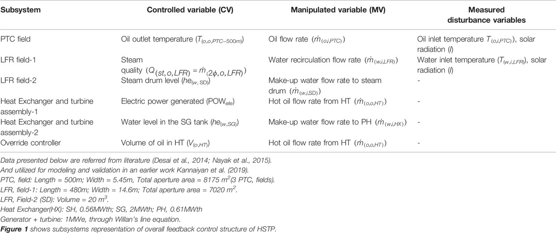
TABLE 1. Summary of controlled, manipulated and measured disturbance variables and override controller for HSTP.

3 Control Objectives of Hybrid Solar Thermal Power Plant

The control objectives of the three subsystems of the HSTP are discussed in this section. The specific objectives for PTC are as follows:

• Oil temperature at outlet of PTC (T_{(o,o,PTC−500m)}) should be at a desired setpoint, irrespective of disturbances such as variations in the wind speed, temperature of oil at the inlet, and the incident solar radiation. Such regulation of heat gain of oil in PTC at a certain level helps avoid thermal stresses and oil leakage.

The control objectives of LFR based Direct Steam Generation (DSG) field are as:

• For DSG, the primary task is to regulate the quality of the water-steam mixture flowing out of LFR (Q_(st,o,LFR)) by manipulating the inlet water flow $({\dot{m}}_{(w,i,LFR)})$ through LFR, irrespective of variations in the solar radiation and input conditions.

• Control of water level in SD is needed to avoid overflow or emptying out of the SD vessel. This water level is maintained by manipulating the makeup freshwater flow into SD $({\dot{m}}_{(w,i,\mathrm{SD})})$.

The control objectives for the HX subsystem are as follows:

• The flow rate and conditions of the steam generated by the HX train are functions of the heat exchanged with the oil (incase of PTC) or the heat received from the reflector (in case of LFR). With increase in oil flow rate to HX $({\dot{m}}_{(o,i,HX)})$, rate of steam generation $({\dot{m}}_{(st,gen,SG)})$ is increased in SG. Also, the combined exit flow of steam from SG and SD is made to flow through SH, where there is a rise in temperature of steam due to increased oil flow rate. The steam from the SH goes to the turbine and generator assembly for electric power generation. The power generated is a function of the steam flow and its properties as stated by Willan’s line equation (Desai et al., 2014; Kannaiyan et al., 2019). The main aim of the HX subsystem is to ensure the production of desired amount of power. In the current work, this is accomplished by choosing oil flow through HX $({\dot{m}}_{(o,i,HX)})$ as manipulated variable and electric power (POW_ele) generated as the controlled variable. The control system should be able to deliver the desired power level in face of various disturbances. In particular, disturbances such as the temperature of oil and water flowing into the HX have a significant bearing on the control loop performance.

• The inventory of water in the SG must be controlled to ensure that the tube bundle carrying the hot oil is always immersed in water to prevent damage to the tubes. Also, controlling the water inventory in SG helps avoid possibility of steam generation in PH itself.

The control objectives for the HT with override control are as follows:

• The HSTP has been designed for daily startup and shutdown, ideally corresponding to sunrise and sunset, respectively. The presence of uncertainties such as cloud cover, coupled with a relatively small thermal storage can result in an unexpected plant shutdown even during the daytime. A well designed control system should minimize such shutdowns and also ensure that the plant fully utilizes the thermal energy before shutdown. Towards this end, the control configuration needs to be changed using an override structure when certain conditions are met.

4 Control Relevant Modeling of Hybrid Solar Thermal Power Plant

A first principles based dynamic model of the HSTP is available in literature (Kannaiyan et al., 2019). However, it is too detailed for the design of a regulatory control system. Typically, control relevant, linear time invariant models in the form of transfer functions that serve as a proxy for the plant are first identified from plant data. Towards this end, in the current work, we treat the first principles literature model (Kannaiyan et al., 2019) as the plant and hence the source of measurements. Each manipulated input (see Table 1) is given step perturbations to obtain the classical process reaction curve of the corresponding controlled variables. During this exercise, the various disturbances listed in Supplementary Table S1 are kept constant. Based on the resulting input-output data, appropriate transfer functions are obtained around the operating point. The list of these candidate transfer functions considered in this work are given in Table 2.

TABLE 2

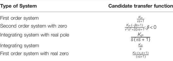
TABLE 2. Candidate transfer functions for HSTP.

The parameters of the transfer function under consideration were obtained using the system identification toolbox in MATLAB 2012a. The best fit model is obtained by minimizing the error between predicted and measured value from the plant. The corresponding percentage fit of a transfer function is obtained by Eq. 1 (Wibowo et al., 2009).

$F{t}_{TF}=\left(1-\frac{\sum _{i=1}^{t_p}|\left(Y{m}_i-{\widetilde{Ys}}_i\right)|}{\sum _{i=1}^{t_p}|\left(Y{m}_i-\overline{Ym}\right)|}\right)\times 100(1)$

In the above equation ${\widetilde{Ys}}_i$ represents the predicted (fitted) model output at time instant i. $Y{m}_i,\overline{Ym}$ represents output measured from plant at time instant i and the mean value of measured output respectively. The data is collected for t_p instants with sampling interval of 1 s. The transfer functions identified for various subsystems and the corresponding fit errors (Eq. (1)) are listed in Table 3. It can be seen from this Table that transfer functions fit the data quite well for most of the subsystems. Figure 2 depicts the step response of the fitted transfer functions and the plant for the various control loops under consideration. These two curves visually show a good match for the various control loops.

TABLE 3

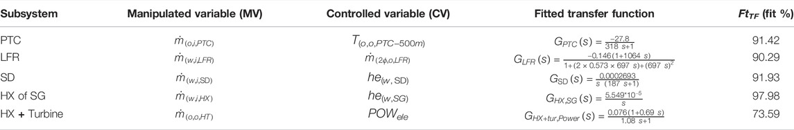
TABLE 3. System identification of HSTP subsystems.

FIGURE 2

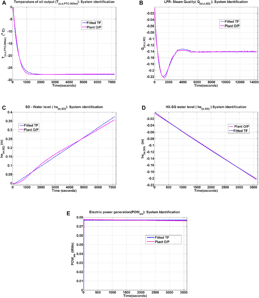
FIGURE 2. System identification of HSTP (A) PTC (B) LFR (C) SD (D) HX-SG level (E) Electric power.

5 Controller Design for Hybrid Solar Thermal Power Plant

Based on the identified control relevant models as summarized in Table 3, conventional PI and PID-type controllers are now designed to ensure disturbance rejection as well as setpoint tracking for the various controlled variable-manipulated variable pairings. The PID controller form, feedback controller tuning, and feedforward controller design used in the HSTP are discussed next.

5.1 Digital PID Controller Design

The velocity form of the PID controller has been used in this work. The velocity form of PID controller has an advantage of no integral windup problems. Moreover, the controller output stays at its previous value in case of failure in the hardware device (Stephanopoulos, 1984). The velocity form of PID controller is obtained by elaborating the difference equation, Δu(k) = u(k) − u (k − 1), where u(k) is the manipulated variable value at the kth sampling instant with sampling interval being T_o as (Stephanopoulos, 1984):

$\begin{array}{ccc}\hfill \mathrm{\Delta }u\left(k\right)& =\hfill & q_{o}e\left(k\right)+q_{1}e\left(k-1\right)+q_{2}e\left(k-2\right)\hfill \\ \hfill \text{where,}{q}_0=K_c\left(1+\frac{{\tau }_d}{T_o}+\frac{T_o}{{\tau }_i}\right);& \hfill & q_1=-K_c\left(1+2\frac{{\tau }_d}{T_o}\right);q_2=K_c\left(\frac{{\tau }_d}{T_o}\right)\hfill \end{array}(2)$

with e(k) = y_sp(k) − y(k) being the set-point tracking error at instant k, and K_c, τ_i, τ_d are the proportional gain, integral time constant, and derivative time constant, respectively.

5.2 Controller Tuning

Several tuning algorithms are available for control system design and are based on the form of the transfer function used to approximate the plant behaviour. In the current work, Internal Model Control (IMC) is employed for the HSTP, since it explicitly uses the desired closed-loop response and the specific form of the transfer function model used to approximate the plant, in order to obtain the controller parameters. The corresponding tuning rules to obtain controller parameters, namely K_c, τ_i, and τ_d, depending on the form of the transfer function used for the components of the HSTP, are outlined in Supplementary Table S2 in SI (Rivera, 1999; Bequette, 2003). The numerical values of the various tuning parameters for the PID controllers, which represent the designed controllers for the HSTP, are summarized in Table 4. For the sake of simplicity, the SD controller tuning was obtained by ignoring the left half pole of the process transfer function. The process and instrumentation diagram depicting these feedback controllers for the HSTP is shown in Figure 1. The manipulated variables in each subsystem have saturation limits and these values used for HSTP are shown in Supplementary Table S3 in SI.

TABLE 4

TABLE 4. HSTP control loop tuning values.

In order to account for the measured disturbances the feedback PID controllers are combined with Static Feed Forward controllers (SFF). Setpoint tracking is handled by feedback controller in a better manner and disturbance rejection is handled by SFF once the disturbance measurement are obtained. Combination of feedback and feedforward control on HSTP components helps to ultimately achieve the electrical demand target. The feedforward controllers based on steady-state balances for the various control loops of the HSTP and their integration with feedback control is discussed next.

5.3 Controller Design for Parabolic Trough Collector

The control problem for the PTC subsystem consists of controlling the outlet oil temperature by manipulating the oil flow rate through the PTC. The feedback block diagram for the PTC is shown in Figure 3A.

FIGURE 3

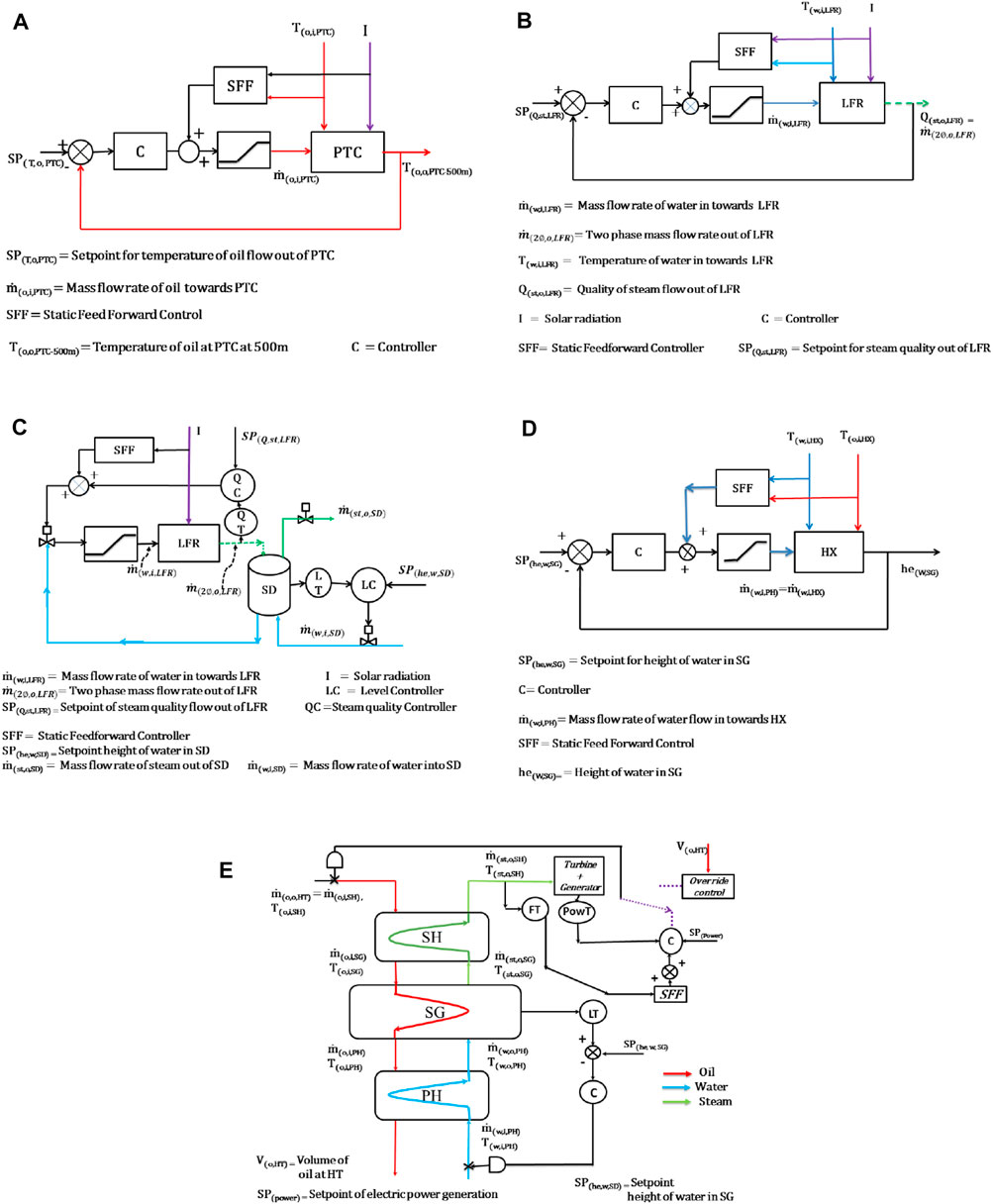
FIGURE 3. Control structures of HSTP (A) PTC (B) LFR (C) LFR + SD (D) HX- SG level (E) Override and electric power.

Feedforward control design for PTC: Availability of measurements of disturbance variables such as solar radiation (I) and inlet temperature of oil (T_(o,i,PTC)) enables implementation of feedforward control in addition to the feedback controller. A steady-state energy balance relates the oil flow rate to solar radiation and inlet oil temperature (equivalently enthalpy) as follows:

$\begin{array}{ccc}\hfill {\dot{m}}_{\left(o,i,PTC\right),FF}\left(h_{\left(o,o,PTC\right)}-h_{\left(o,i,PTC\right)}\right)& =\hfill & IA{\eta }_{\left(opt,PTC\right)}\hfill \\ \hfill \Rightarrow {\dot{m}}_{\left(o,i,PTC\right),FF}& =\hfill & \frac{IA{\eta }_{\left(opt,PTC\right)}}{\left(S{P}_{\left(h,o,PTC\right)}-h_{\left(o,i,PTC\right)}\right)}\hfill \end{array}(3)$

where SP_(h,o,PTC) is the enthalpy of the oil exiting the PTC corresponding to the temperature setpoint SP_(T,o,PTC) of PTC. The Static FeedForward controller (SFF) calculation block as depicted in Figure 3A uses Eq. 3 as the feedforward law. The oil flow rate computed by the feedforward law is then added to the flow rate computed by the feedback component to determine the net oil inlet flow rate through the PTC receiver tubes.

5.4 Controller Design for Direct Steam Generation

In the HSTP reported in this work, direct steam generation is based on LFR receiver tubes and the steam drum. LFR control involves controlling the quality of steam flowing out of LFR (Q_(st,o,LFR)) by manipulating the water flow $({\dot{m}}_{(w,i,LFR)})$ through LFR. Quality of steam inherently represents the mass flow rate of steam out of LFR $({\dot{m}}_{(st,o,LFR)}=Q_{(st,o,LFR)}\times {\dot{m}}_{(w,i,LFR)})$, as well as mass flow rate of water out of LFR $({\dot{m}}_{(w,o,LFR)}=(1-Q_{(st,o,LFR)})\times {\dot{m}}_{(w,i,LFR)})$. The feedback block diagrams for LFR, and LFR + SD are shown in Figures 3B,C, respectively.

Feedforward control design for LFR: Measurements of disturbances such as solar radiation, temperature (or equivalently, enthalpy) of water flowing into LFR and water and steam exiting LFR (I, h_(w,i,LFR), h_(w,o,LFR), h_(st,o,LFR)), can be used to obtain a feedforward control law. This is based on steady-state energy balance as follows,

$\begin{array}{ll}\hfill & \left({\dot{m}}_{\left(st,o,LFR\right)}{h}_{\left(st,o,LFR\right)}+{\dot{m}}_{\left(w,o,LFR\right)}{h}_{\left(w,o,LFR\right)}\right)-\left({\dot{m}}_{\left(w,i,LFR\right),FF}{h}_{\left(w,i,LFR\right)}\right)=\left(IA{\eta }_{\left(opt,LFR\right)}\right)\hfill \\ \hfill \Rightarrow & {\dot{m}}_{\left(w,i,LFR\right),FF}=-\frac{L_{FF}}{h_{\left(w,i,LFR\right)}}\hfill \\ \hfill & \text{where},L_{FF}=\left(IA{\eta }_{\left(opt,LFR\right)}\right)-\left(S{P}_{\left(Q,st,LFR\right)}{\dot{m}}_{\left(w,i,LFR\right)}{h}_{\left(st,o,LFR\right)}\right)-\left({\dot{m}}_{\left(w,o,LFR\right)}{h}_{\left(w,o,LFR\right)}\right)\hfill \end{array}(4)$

In above, SP_(Q,st,LFR) represents the setpoint of LFR. The SFF calculation block in Figure 3B is based on Eq. 4, which is then combined with the output of the feedback PID controller to obtain the resultant manipulated variable for control of LFR steam quality.

5.5 Controller Design for Heat Exchanger and Turbine Assembly

Maintaining height of water level in SG (he_(w,SG)) is essential to maintain its operating pressure to facilitate electric power generation. Water level control of SG is obtained by manipulating water flow rate flowing into the PH $({\dot{m}}_{(w,i,HX)})$, since it is same as water flow rate entering SG $({\dot{m}}_{(w,i,SG)})$. In the beginning, in both open-loop and closed-loop operations, the generated steam is accumulated till pressure of SG (P_SG) rise to its rated pressure (40 bar in the current work). Once pressure of SG reaches or is greater than the rated operating pressure, closed-loop control operation starts by manipulating variable $({\dot{m}}_{(w,i,HX)})$ for keeping he_(w,SG) constant. Since the flow rate of steam generation and flow rate of water flow into SG are not equal, minor variations (of 0.5 bar i.e. 39.5–40.0 bar) in pressure values are considered acceptable for allowing mass flow rate of steam to exit SG. The feedback control for height of water level control of SG and its block diagram is shown in Figure 3D. The steam generated in SG varies due to variations in temperature and flow rate of oil entering the HX assembly. This in turn affects water level. So, the feedback action is augmented with feedforward control to facilitate meeting the electric demand.

Feedforward control element for heat exchanger: A static feedfoward control for HX was designed to compensate for disturbance variables such as enthalpy of water flowing in and enthalpy of oil flowing into HX (h_(w,i,HX), h_(o,i,HX)). The computation of mass flow rate of oil into HX $({\dot{m}}_{(o,i,HX)})$ needed to generate the target electric power consists of two steps. First, mass flow rate of steam exiting the steam generator $({\dot{m}}_{(st,o,SG)})$ for a given power level is computed using Willan’s line equation (Desai et al., 2014) as:

$PO{W}_{\mathit{act,ele}}=\left(a+b{\dot{m}}_{\left(st,o,SH\right)}\right)X_P{X}_T(5)$

where ${\dot{m}}_{(st,o,SH)}={\dot{m}}_{(st,o,\mathrm{SD})}+{\dot{m}}_{(st,o,SG)}$ is the total flow rate of the steam exiting the super heater, and X_P, X_T represent the correction factors for steam pressure and steam temperature respectively (Desai et al., 2014). Substituting for ${\dot{m}}_{(st,o,SH)}$ in Eq. (5), and replacing POW_act,ele with the power setpoint (SP_(power)), we get the flow rate of steam exiting the steam generator computed by feedforward control action to be:

${\dot{m}}_{\left(st,o,SG\right)}=\frac{S{P}_{\left(power\right)}-a{X}_P{X}_T-b{\dot{m}}_{\left(st,o,\mathrm{SD}\right)}{X}_P{X}_T}{b{X}_P{X}_T}(6)$

As a second step, the mass flow rate of oil $({\dot{m}}_{(o,i,HX)})$ into the HX is computed as follows:

$\begin{array}{ccc}\hfill {\dot{m}}_{\left(o,i,HX\right)}\left(h_{\left(o,i,HX\right)}-h_{\left(o,o,HX\right)}\right)& =\hfill & {\dot{m}}_{\left(w,i,HX\right)}\left(h_{\left(st,o,HX\right)}-h_{\left(w,i,HX\right)}\right)\hfill \\ \hfill \Rightarrow {\dot{m}}_{\left(o,i,HX\right)}& =\hfill & \frac{{\dot{m}}_{\left(w,i,HX\right)}\left(h_{\left(st,o,HX\right)}-h_{\left(w,i,HX\right)}\right)}{\left(h_{\left(o,i,HX\right)}-h_{\left(o,o,HX\right)}\right)}\hfill \end{array}(7)$

In the above equation the steam generated by SD has not been considered. Thus, h_(st,o,HX) represents the enthalpy at the exit of superheater of the steam generated only by the SG. Further, it is assumed that the level of water in SG is maintained constant i.e. ${\dot{m}}_{(st,o,SG)}={\dot{m}}_{(w,i,SG)}$. Eq. (7) is implemented using the SFF calculation block as shown in the block diagram in Figure 3E. The feedforward controller computed oil flow rate is added to the PI controller output to obtain the net hot oil flow rate to be sent to the HX.

It is to be noted that power computed by Willan’s equation (Eq. (5)) can be negative since coefficient a is negative (refer to Supplementary Table S4 in SI). To avoid negative power computation, the power generated by the turbine is computed as:

$PO{W}_{\mathit{ele}}=MAX\left(0,PO{W}_{\mathit{act,ele}}\right)(8)$

Further details about Willan’s equation and generation of electric power are presented in Section 3 in SI.

5.6 Override Control Strategy

The HSTP has been designed for daily startup and shutdown, ideally corresponding to sunrise and sunset, respectively. Presence of uncertainties such as cloud cover and the relatively small thermal storage can result in unexpected plant shutdown. Thus, the control system must ensure that the plant fully utilizes the thermal energy before shutdown. To this end, the control configuration needs to be changed using an override structure when certain conditions are met. In the proposed override control strategy, oil flow rate from HT tank $({\dot{m}}_{(o,o,HT)})$ is set by the controller controlling the power level when the volume of oil in HT is within certain limits (low and high).

The sequence of operation for override control action between the HX and HT subsystems is as shown in Figure 4 and Table 5. In this operation the control signal for the hot oil flow rate could be obtained in three different ways: 1) Manipulated Variable (MV) from PI control (U_fb) 2) High flow rate of oil flow out of HT $(H_{{\dot{m}}_{(o,o,HT)}})$ to prevent further increase in oil volume, when the HT is close to being full, and 3) Low flow rate of oil flow out of HT $(L_{{\dot{m}}_{(o,o,HT)}})$ to prevent further decrease in oil volume, when the HT is close to being empty. Depending upon the region of volume of oil in HT as well as the trend of oil level change, these options of flow rates are triggered as follows (refer Figure 4).

• Region A to B: Volume of oil in this region is high, and hence the flow rate of oil exiting the HT tank is kept at the maximum value. This value depends on the mass flow rate of oil into HT $({\dot{m}}_{(o,i,HT)})$ and maximum allowed oil flow rate out of HT $(H_{{\dot{m}}_{(o,o,HT)}})$.

• Region B to C: Volume of oil in this region is adequate, so PI controller (U_fb) of the electric power control loop decides the flow rate of oil flowing out of HT.

• Region C to D: Volume of oil in this region is low but still, PI controller (U_fb) decides the flow rate of oil flowing out of HT.

• Region D to E: Volume of oil is approaching adequate volume region. However, to ensure sufficient oil accumulates, the flow rate of oil flow through HX is minimum of the minimum (lowest possible) oil flow rate out of HT tank $(L_{{\dot{m}}_{(o,o,HT)}})$ and flow rate demanded by feedback controller (U_fb).

• Region E to F: Volume of oil in this region is adequate and hence PI controller decides the flow rate of oil flow out of HT.

• Region F to G: Volume of oil is approaching high volume region but still PI controller decides the flow rate of oil flow out of HT.

FIGURE 4

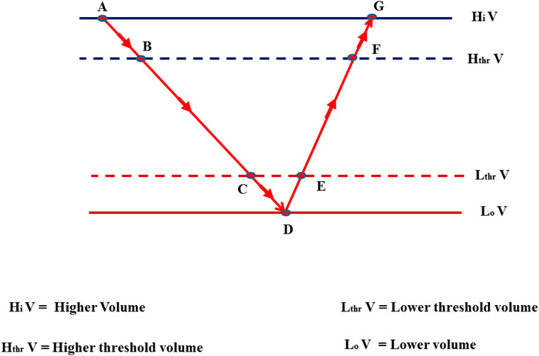
FIGURE 4. Block diagram for override control action for HX.

TABLE 5

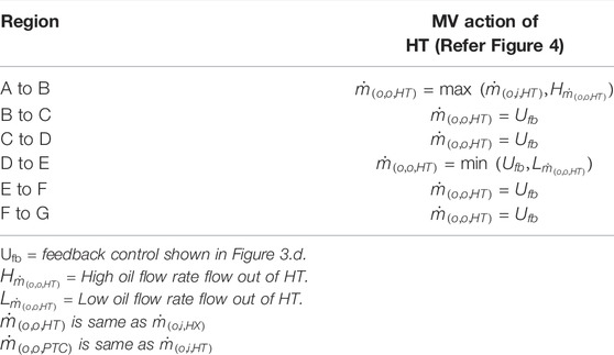
TABLE 5. Override control operation.

Different decision making for flow rate in regions A to B, and F to G, has been designed to reduce chattering of the oil flow rate near the high threshold volume (B or F). Similar is the case for the lower volume band (region C to D, and D to E). If the volume of oil is on higher side of region A, maximum of $\left.(U_{fb},H_{{\dot{m}}_{(o,o,HT)}}\right)$ is activated, whereas if the volume of oil becomes lower than value D, minimum of $(U_{fb},L_{{\dot{m}}_{(o,o,HT)}})$ action is activated.

The feedback controllers, along with the feedforward elements and the override control constitute the proposed regulatory control layer for closed-loop operation of the HSTP. We next present two case studies demonstrating the utility of the proposed closed-loop operation vis-a-vis open-loop operation.

6 Case Study I: Plantwide Control Case Study of Hybrid Solar Thermal Power Plant

In this section, we present a simulation case study to demonstrate the utility of the control layer. This case study has a quadratic solar radiation profile with cloud cover as shown in Figure 5. The Open-Loop (OL) simulation with similar solar radiation and the corresponding HSTP performance has been discussed in detail in our earlier work (Kannaiyan et al., 2019). The performance in OL is shown using dotted lines in Figures 7–18. The solar radiation profile for this case study is shown in Figure 5. It can be seen that in this profile, maximum solar radiation of approximately 800 W/m² is obtained at 2 h 45 min. Further, apart from varying significantly throughout the day, the solar radiation also has a significant drop for about 15 minutes after around 4 hours, corresponding to a cloud cover scenario. In particular, the solar radiation drops from 690 to 300 W/m² for about 900 s and then again rises from 300 to 620 W/m² as shown in Figure 5. During field operations, such scenarios can occur frequently, and it is of interest to assess the ability of the control system to ensure continuous electric power generation in presence of such variations. In this closed-loop controller implementation case study, initial conditions for HSTP are similar to open–loop simulation of a cold startup as given in Table 6 (Kannaiyan et al., 2019).

FIGURE 5

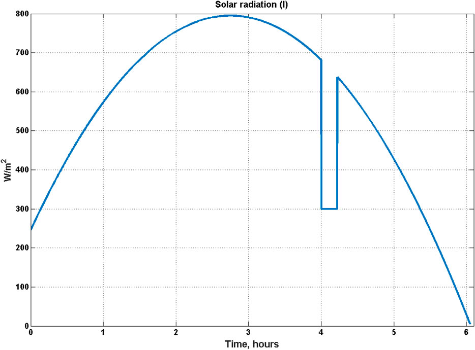
FIGURE 5. Quadratic solar radiation profile.

TABLE 6

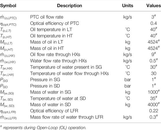
TABLE 6. Case study I and Case study II: Initial conditions, parameters and input variables.

Before presenting the results, we first discuss a few operational details related to both open and closed-loop operation:

• Before starting the HSTP, the initial conditions for the plant are specified as discussed in Table 6. Once the pressure in SG or SD attains the required operating pressure, steam is allowed to flow from SG and SD through SH to the turbine for electric power generation. Electric power generation after sufficient pressure build-up in SD starts at about 1 h 57 min while the plant is being operated in open-loop mode. Closed-loop control operation is activated for overall HSTP at about 2 h 45 min once the pressure in SG attains 40 bar. Thus, the plant is under closed-loop control operation from 2 h 45 min to 6 h 02 min for quadratic solar radiation. Shutdown of HSTP is triggered if the temperature of the oil from PTC or HT is less than 300 °C for 5 min continuously, or when volume of oil in HT (V_(o,HT)) reduces to less than 1.5 m³ (lower threshold volume of oil at HT as shown in Figure 4) for 10 min continuously. From Figure 6, it can be seen that the shutdown in the open-loop and closed-loop operation is triggered at different times based on volume of oil in HT and temperature of oil out of PTC. The closed-loop operation was simulated in MATLAB version 2018A running on windows operating system on a computer with 32 GB RAM and Intel-core i7 processor.

• Setpoints: Overall control structure of HSTP is summarized in Figure 1 and it consists of five control loops. Setpoint computation for closed-loop control of PTC, LFR, SG, SD, and electric power generation as shown in Table 7 is discussed below:

1. PTC field: Temperature rise of oil at PTC exit was maintained within the range of 100 °C so as to minimize heat losses to the atmosphere. This is similar to strategies followed in literature (80 °C in Camacho and Gallego, (2013) and 110 °C in Wittmann et al. (2009)). The PTC oil outlet temperature setpoint is computed and updated every 30 min as shown in Table 7.

2. LFR: Based on an aperture area of 7,020 m², the steam quality setpoint in LFR is maintained at 35%. This ensures safe operation and minimizes heat loss (Desai et al., 2014; Nayak et al., 2015).

3. SD: By maintaining the mass of water at 50% in SD, the level of water is maintained at 0.9 m. This condition enables us to drive DSG with sufficient thermal energy and mass inventory (Eck and Hirsch, 2007). The level of water is controlled in the steam drum, since maintenance of the level ensures required pressure in SD along with ensuring that the thermal variables are maintained within the limits.

4. SG: Level setpoint is set at 0.4 m based on the dimension of SG as shown in Table 7.

5. Electric Power: The setpoint is set to 60% of the maximum capacity (1 MWe) of electric power generation of the HSTP.

FIGURE 6

FIGURE 6. Open-loop and closed-loop operating strategies for HSTP.

TABLE 7

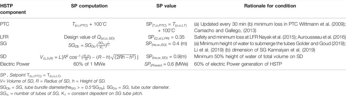
TABLE 7. Setpoints for closed-loop control operation of HSTP.

The controller settings are given in Table 4. Details of tuning rules and manipulated variables limits are shown in SI (Supplementary Table S3).

6.1 PTC

The performance of PTC for open and closed-loop operations is shown in Figure 7. The startup implementation is discussed in Kannaiyan et al. (2019). When the pressure in the SG reaches 39.5 bar, the condition for transfer to automatic control is met and the plant is subsequently operated in closed-loop. The time of this transfer depends on the prevailing solar radiation and was found to be at 2 h 45 min after startup. As can be seen from Figure 7 (top panel), heat gain by oil is more during this period, and this time also corresponds to peak solar radiation. The mass flow rate of oil entering the PTC $({\dot{m}}_{(o,i,PTC)})$ is the manipulated variable used to track the target oil temperature setpoint. The initial increase in oil flow rate as determined by the PI controller results in the saturation of oil flow rate and a drop in the temperature from 350 to 304 °C is observed. From 4 to 4 h 12 min, solar radiation drops due to the onset of the cloud cover episode. The temperature of oil exiting the PTC (T_{(o,o,PTC−500m)}) rises by about 3.6% while mass flow rate of oil flowing out of PTC $({\dot{m}}_{(o,i,PTC)})$ reduces from 3 to 0.5 kg/s which is the lower saturation limit. During the solar radiation rise period when the cloud cover episode ends, T_{(o,o,PTC−500m)} drops from 341 to 309 °C while ${\dot{m}}_{(o,i,PTC)}$ increases from 0.5 to 6.95 kg/s. PTC receives oil from LT tank. As the oil outlet temperature of LT tank (T_(o,o,LT)) varies, so does the oil temperature of the inlet flow to PTC (T_(o,i,PTC)). Hence setpoint is updated every 30 min for PTC as mentioned in Table 7 and shown in Figure 7. Maximum setpoint change occurs at 3 h 15 min where it decreases by 6.6%. Other setpoint variations are of less than 1.5% magnitude. It can be noted from Figure 7 (top panel) that the controller is able to significantly reduce the effect of disturbance in the solar radiation by manipulating the oil flow rate (bottom panel). However, the PTC outlet temperature in the open-loop operation (top panel in Figure 7) drops significantly after the onset of cloud cover and the plant is subsequently shutdown due to the triggering of shutdown conditions. The oil flow rate through PTC is maintained constant at 3 kg/s (bottom panel in Figure 7) in the open-loop operation.

FIGURE 7

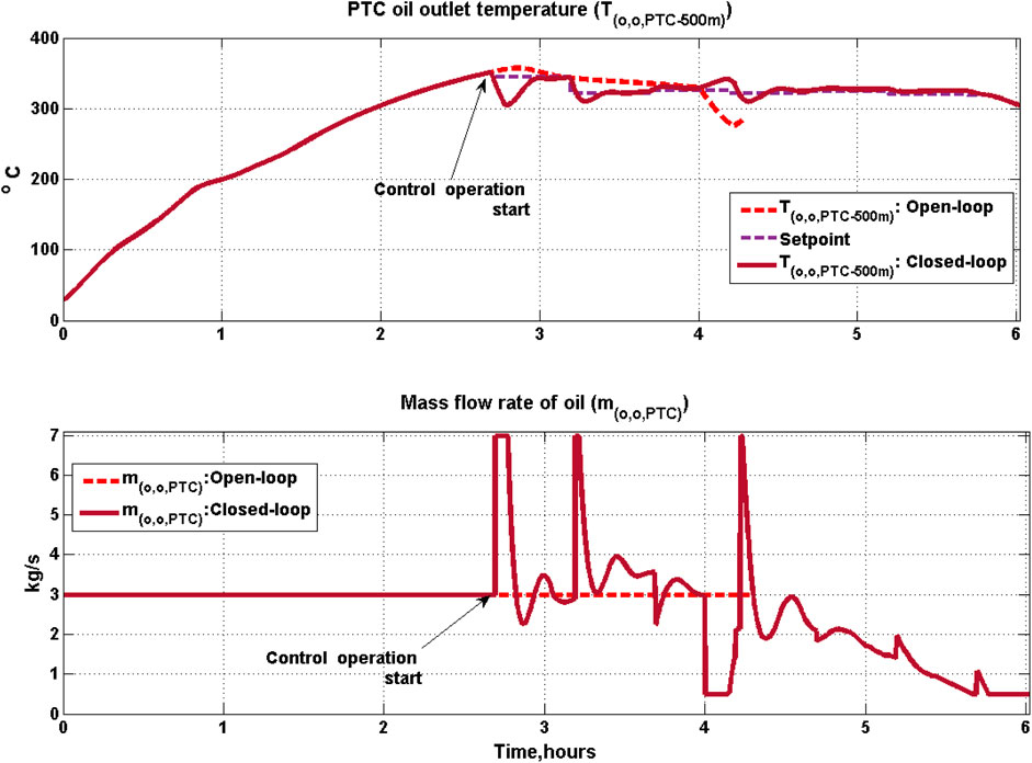
FIGURE 7. PTC control: Closed-loop and open-loop profile of PTC.

The average thermal efficiency (as shown in Eq. (9)) obtained for PTC is 0.80 for 6 h 02 min of overall plant operation for the closed-loop based on setpoint update mechanism, while in open-loop it was 0.81 but only for 4 h 17 min operation.

6.2 HT

High Temperature Tank (HT) serves as the hot oil inventory which can be used to operate the plant, providing constant electricity, even in presence of events such as a passing cloud cover or fluctuating solar radiation. However, for safety and equipment integrity, the volume of oil present in the HT (V_(o,HT)) has to be maintained within the specified limits (1.5–8 m³). Since the HXs do not provide for the accumulation of oil, the mass flow rate of oil through the train of HXs (SH, SG, PH) is at the same value as the mass flow rate of oil flow out of HT $({\dot{m}}_{(o,o,HT)})$. The profile of mass and enthalpy of oil in the HT can be seen in Figure 8. This figure also shows the profiles of these variables for the LT tank. The corresponding volume of oil in the HT is shown in Figure 9. It can be seen from Figure 8 (upper panel) that the mass of the oil in the HT increases after the start of control operation. The corresponding volume of oil stored in HT also increases (bottom panel, Figure 9). This is due to the higher flow rate of oil from PTC (Figure 7) due to high solar radiation, compared to the oil flow rate exiting the HT. Once the volume of oil is in ranges 8 to 7 m³ or 1.5 to 2.5 m³, the override controller takes over. The subsequent fluctuations (between 4 and 5 h 26 min) in the amount of oil volume inventory are caused by the override control strategy. During the cloud cover episode, the disturbance of solar radiation causes relatively lower variation in oil temperature of HT, namely that it rises from 328 to 336°C and drops from 336 to 316°C respectively as shown in Figure 17.

FIGURE 8

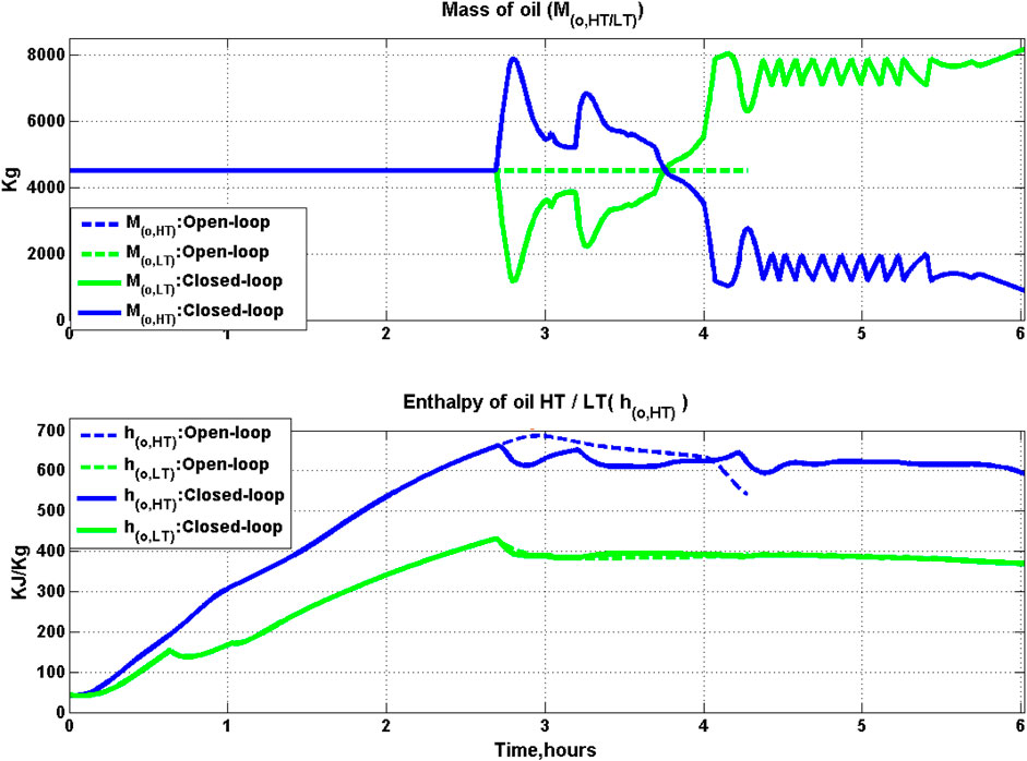
FIGURE 8. Closed-loop and open-loop profile of mass and enthalpy of oil in HT and LT. In the top panel, the dashed blue line corresponding to mass of oil in HT tank in open-loop overlaps with the dashed green line which corresponds to mass of oil in LT tank in open-loop.

FIGURE 9

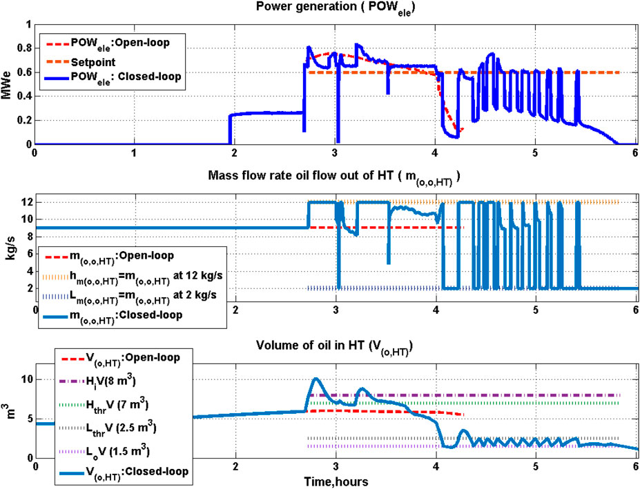
FIGURE 9. Electric power generation of STP in closed-loop and open-loop operation.

It can be further seen that at the onset of cloud cover (at around 4 h), the mass of oil in the HT starts dropping since the oil flow rate coming from the PTC field has dropped while the amount of oil being sent to HX assembly is constant in accordance with the override strategy in Table 5 (middle panel, Figure 9). Volume of oil in HT increases above 8 m³ at 2 h 47 min and 3 h 16 min of closed-loop operation, and during this time ${\dot{m}}_{(o,i,HT)}$ is greater than ${\dot{m}}_{(o,o,HT)}$ even though the outlet flow rate is set at maximum of 12 kg/s for HT. Once the cloud cover episode ends, the mass of oil again increases from 1066 to 2,736 kg (at around 4.2 h), and then it oscillates in a range from 1919 to 1176 kg (4 h 25 min to 5 h 30 min). During shutdown of plant, it reaches the lower mass of 909 kg. Compared to the closed-loop, the mass of oil in the HT does not change in the open-loop operation since the flow rate of oil exiting the HT is the same as the flow rate of oil entering the HT. The variation in the mass of oil in the closed-loop in turn allows power to be produced even during the cloud cover episode as discussed in the next section.

6.3 Power Generation

The HSTP generated electric power profile is shown in Figure 9 (top panel). It can be seen that power is produced for much longer duration for the closed-loop case than for the open-loop case. In particular, the plant is able to generate power even during the cloud cover episode in closed-loop operation. The profile of the manipulated variable for the power loop, namely the oil flow rate exiting the HT is also shown in Figure 9 (middle panel). This flow rate is maintained within the upper and lower limits of 12 and 2 kg/s respectively. The flow rate hits the maximum value at the start of the control operation due to activation of override control since the volume in the HT increases rapidly due to high inlet flow rate from the PTC field because of high solar radiation. The subsequent oscillations in the oil flow rate from about 4 to 5 h 26 min (middle panel, Figure 9) are a manifestation of the interplay between the override action and the PI controller controlling the power output. Based on the override operating strategy as shown in Figure 4, when the volume of oil is varying from C (L_thrV = 2.5 m³ in Figure 9) to D (L_oV = 1.5 m³ in Figure 9), the ${\dot{m}}_{(o,o,HT)}$ value is determined by the power control loop and is set at 12 kg/s. However, the moment the level hits the threshold D, the ${\dot{m}}_{(o,o,HT)}$ value is set by the override action to be equal to 2 kg/s which causes the level to increase. Once the level reaches threshold E, again the same cycle repeats. When volume of oil is in range from 7 to 2.5 m³ (during 3.5–4 h), electric power generation controller is activated and the resultant ${\dot{m}}_{(o,o,HT)}$ takes a value in the range 10.97 to 9.325 kg/s. Once V_(o,HT) hits the lower limit saturation of 1.5 m³, override controller action is triggered which fixes ${\dot{m}}_{(o,o,HT)}$ to 2 kg/s. Thus, both override control and the electric power generation tracking control are active during different periods of operation. As a result, the electric power generated by the HSTP plant oscillates between 0.29 and 0.75 MWe as shown in Figure 9. Shutdown condition is reached once the volume of oil is at 1.5 m³ continuously for 10 min of operation. This happens when solar radiation reduces at end of the day, resulting in triggering of the override control action which sets the oil flow rate from the HT to the lower saturation value of 2 kg/s.

6.4 Steam Generator Level

In the HX assembly, maintenance of Steam Generator (SG) water level at the specified setpoint is necessary to ensure proper operating pressure and variation of thermal variables within the limits as well as ensuring that the tube bundle is immersed in the boiler feedwater. This level is partly determined by the amount of steam generated in the SG which in turn depends on the flow rate and temperature of oil entering the SG. This flow rate $({\dot{m}}_{(o,o,HT)})$ in turn is a manipulated variable for the power block PI controller and hence varies in response to variation in solar radiation. Further, the electrical power generated in HSTP is a function of flow rate of steam entering the turbine (Desai et al., 2014). Thus, there is a complex interplay between power generated and SG level. The SG level is controlled by manipulating the flow rate of water entering the PH $({\dot{m}}_{(w,i,PH)})$ which is the same as the flow rate of water entering the SG $({\dot{m}}_{(w,i,SG)})$. The variations in the SG level and the water flow rate in both closed and open-loop operations are shown in Figure 10. From this Figure, it is seen that level of water is maintained constant using PI controller. The control action leads to fluctuation in water flow rate through PH $({\dot{m}}_{(w,i,PH)})$. As a result, the mass flow rate of steam out of SG $({\dot{m}}_{(st,o,SG)})$ also oscillates. The mass flow rate of oil flowing through HX $({\dot{m}}_{(o,i,HX)})$ also oscillates based on override control or power generated feedback control. As a result, the steam generation inside SG also varies as shown in Figure 11. The volume of shell side of SG (refer Kannaiyan et al. (2019)) is high and hence the fluctuations of the mass flow rate of water into HX $({\dot{m}}_{(w,i,HX)}={\dot{m}}_{(w,i,SG)})$ have a negligible effect on the level or mass of water in SG as shown in Figure 10. The following additional observations can be noted:

• In both open-loop and closed-loop strategies, the pressure in SG is kept constant by setting the amount of steam exiting the SG to be equal to the amount of steam getting generated in the SG. However, fluctuations in mass flow rate of water flowing into SG $({\dot{m}}_{(w,i,SG)})$, lead to oscillations of pressure in SG within a small range of 39.5–40 bar. Steam is allowed to flow out of the SG if the pressure inside the SG is greater than 39.5 bar. This causes fluctuations in flow rate of steam flowing out of SG $({\dot{m}}_{(st,o,SG)})$.

• For the closed-loop operation, the steam generation oscillates in the range 0.83 to 0.07 kg/s as shown in Figure 11. This is in response to variation in the HT exit oil flow rate which results due to interplay between override control and the power control strategies. This in turn causes oscillations in the temperature of oil, water, and steam leaving the heat exchanger as shown in Figures 17, 18.

FIGURE 10

FIGURE 10. HX: Closed-loop and open-loop profile of HX.

FIGURE 11

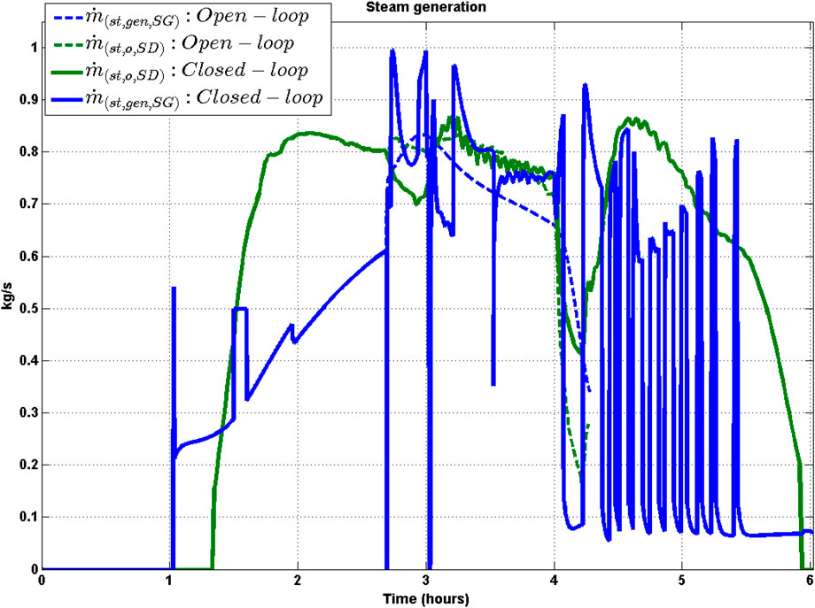
FIGURE 11. Closed-loop and open-loop profile of mass flow rate of steam generation SG and steam out of SD.

6.5 PH and SH

SH and PH are single phase heat exchangers, and no control degrees of freedom are available for these exchangers. Thus, the profile of oil and water/steam out of the HX assembly is affected primarily due to boiler (SG) operation. The temperature of the oil and water/steam profile in the HX assembly is shown in Figures 17, 18 respectively. The performance of oil, water and steam temperature exit out of PH and SH profiles are discussed in detail in Section S4 in SI.

6.6 LFR

The quality of steam flowing out of LFR needs to be maintained constant since this determines the steam quantity that is added to the SG generated steam entering the SH and in turn affects the power generated. This steam flowing out of LFR can be thought of as a disturbance variable for the power generation block. Thus, keeping the LFR steam quality constant reduces the impact of this interaction with the power generation loop. This is achieved by manipulating the flow rate of water entering the LFR $({\dot{m}}_{(w,i,LFR)})$ which should be within limits (0.8–6.4 kg/s) to ensure stability of the two-phase flow. The performance profile of steam quality (steam generation out of LFR (Q_(st,o,LFR))) is shown in Figure 12 (upper panel). The level of water in the SD is controlled by manipulating the freshwater flow rate entering the SD.

FIGURE 12

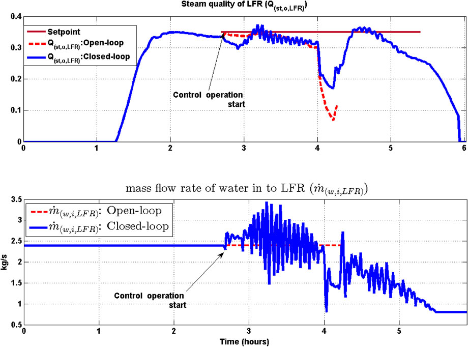
FIGURE 12. LFR: Closed-loop and open-loop profile of LFR.

Following can be observed from Figure 12

• The steam produced by LFR is saturated steam. The steam production from LFR commences at about 1 h 21 min, and the LFR is shutdown at about 6 h 02 min. Thus, total time period of steam production in LFR is about 4 h 41 min.

• During the cloud cover episode, ${\dot{m}}_{(w,i,LFR)}$ drops from 2.39 to 0.8 kg/s which is the lower input limit, and the quality of steam out of LFR (Q_(st,o,LFR)) drops from 0.31 to 0.17. Pressure drop of LFR pipe with reference to inlet pressure of LFR (45 bar) is about 0.6 bar during this period as shown in Figure 13. Average thermal efficiency (Eq. 9) of LFR is obtained as 0.78 for 6 h 02 min of operation.

FIGURE 13

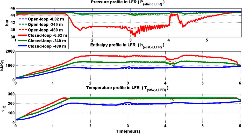
FIGURE 13. LFR profile in closed-loop and open-loop: (a) Pressure (b) Enthalpy (c) Temperature.

6.7 SD

The level of the water in the SD varies due to variation in the flow rate of water entering the LFR as well as the quality of the steam exiting the LFR. The profile of SD water level and freshwater flow rate into SD is shown in Figure 14. It is seen from Figure 14 (lower panel) that during the cloud cover episode, the mass flow rate of water flowing in towards SD $({\dot{m}}_{(w,i,\mathrm{SD})})$ varies from 0.77 to 0.4 kg/s during drop period and again rises from 0.4 to 0.882 kg/s when the episode gets over. The corresponding pressure in SD (P_SD) also varies from 69 to 48.45 bar (Figure 15) during the onset of cloud cover and rises from 48.45 to 77.48 bar at the end of the cloud cover episode as shown in Figure 15. The mass of steam present inside SD varies from 69.5 to 47.89 kg during solar radiation drop and during solar radiation rise period, it increases to 76 kg as shown in Figure 16. The temperature of water present in the SD is almost constant during open-loop and closed-loop operation of SD as shown in Figure 16. In open-loop operation, water is replenished to SD at the same rate as the mass flow rate of steam flowing out of SD.

FIGURE 14

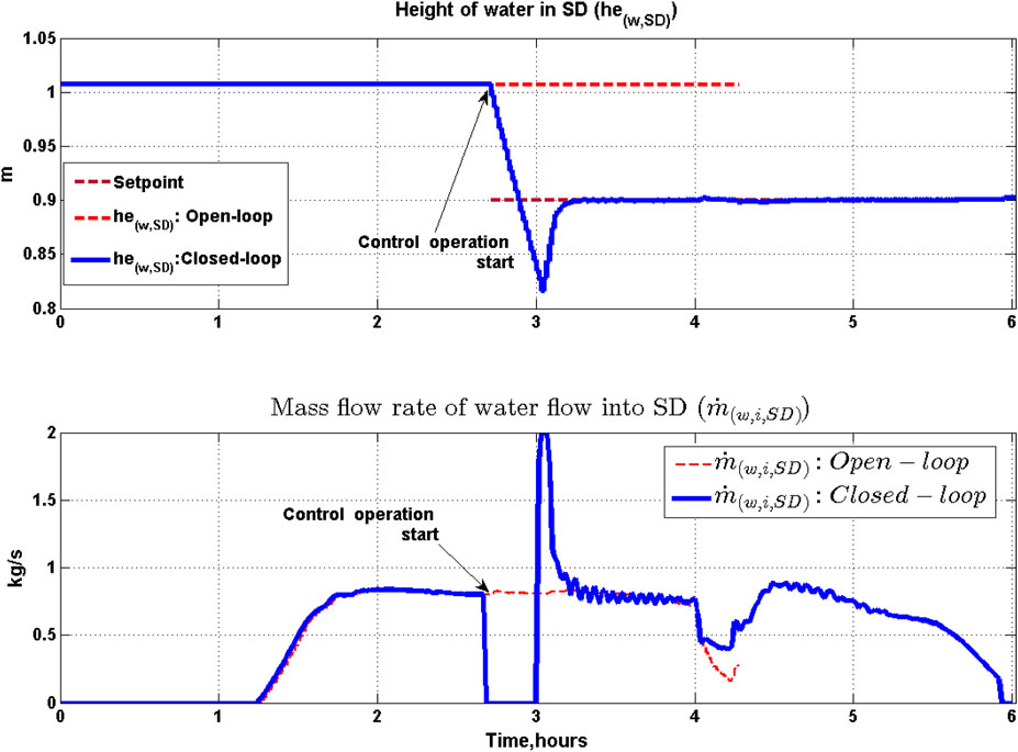
FIGURE 14. SD: Closed-loop and open-loop profile of SD.

FIGURE 15

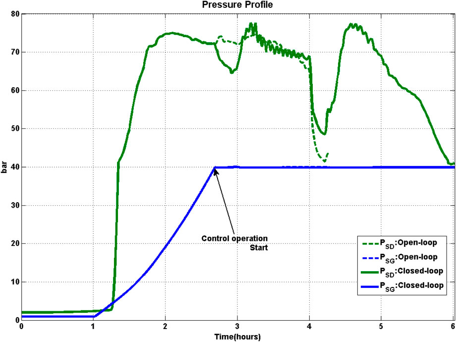
FIGURE 15. Pressure profile of SG and SD in closed-loop and open-loop.

FIGURE 16

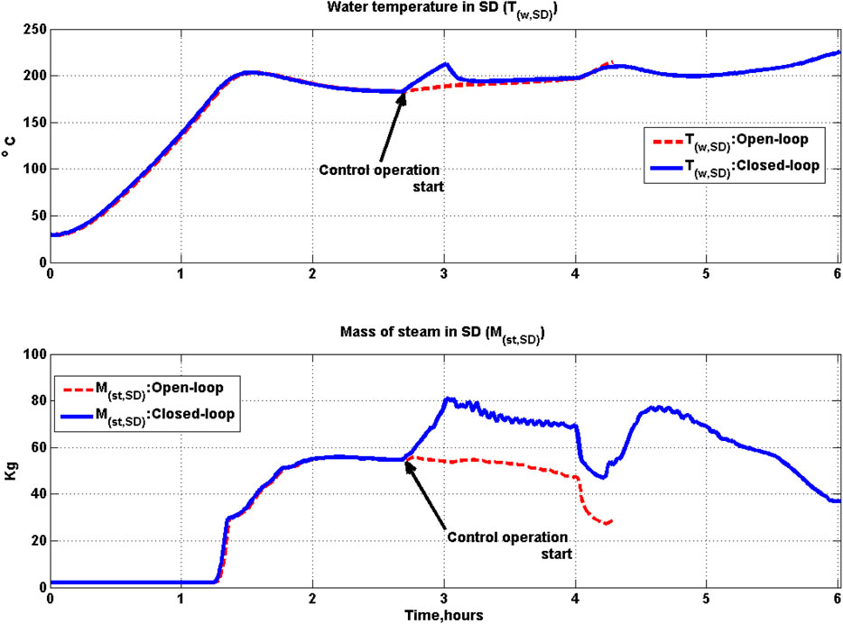
FIGURE 16. SD: Closed-loop and open-loop profile of temperature of water and mass of steam in SD.

6.8 Overall Plant

The oil temperature profiles and water/steam temperature profiles of HSTP are shown in Figures 17, 18 respectively for both open and closed-loop operation. From Figure 17 it is seen that at the instant of shutdown the HT oil temperature is at 293°C for the open-loop operation (at 4.2 h), while it is at 324°C for the closed-loop control operation at the same time. Another interesting observation is that in both open and closed-loop operations, the HT oil temperature is greater than the PTC outlet oil temperature at shutdown. Thus, HT holds some energy during shutdown which gets utilized during startup next day as case study-II presented later in Section 7 demonstrates.

FIGURE 17

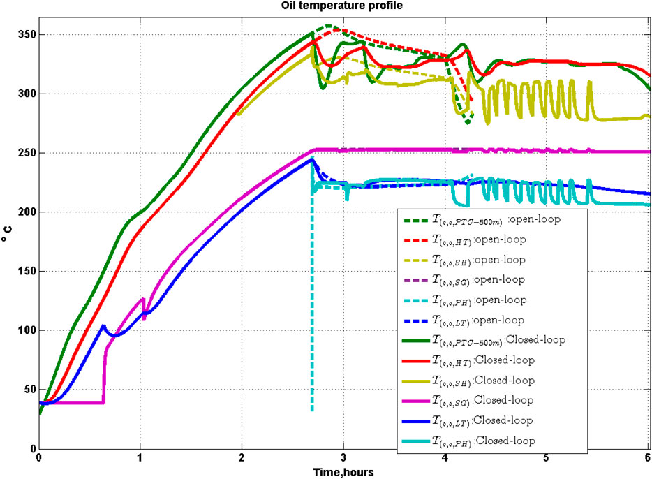
FIGURE 17. Closed-loop and open-loop profile of oil temperature.

FIGURE 18

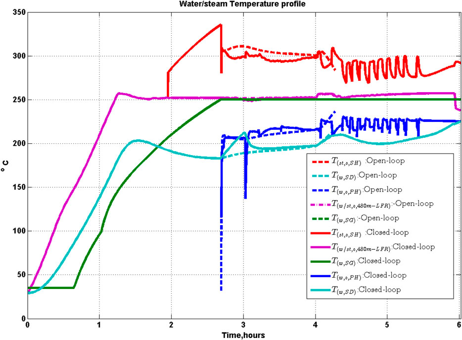
FIGURE 18. Closed-loop and open-loop profile of water/steam temperature.

Temperature rise in PTC in closed-loop operation is less compared to open-loop operation during 3–4 h 17 min operation period. Resultant temperature variation of oil flow into HX (T_(o,i,HX)) is lesser compared to open-loop operation. This in turn leads to less oscillations of the mass flow rate of oil out of HT $({\dot{m}}_{(o,o,HT)})$ during this time period and hence the temperature profile of further stages in HX is not affected. In particular, since the variation of temperature of the oil is lesser in closed-loop operation, water and steam temperature is also affected to a lesser degree in closed-loop operation compared to open-loop operation as shown in Figure 18. During the trailing edge of solar radiation from about 4 to 6 h 02 min operation period in closed-loop operation, temperature of oil out of PTC, HT and SG are almost constant. On the other hand, in the open-loop operation the temperatures decrease significantly during 4–4 h 20 min of operation as shown in Figure 17. Similarly, the temperature of water/steam out of SH, SG, and PH is almost constant in closed-loop operation, while in the open-loop operation the corresponding temperatures show significant variation (Figure 18).

The thermal efficiency of PTC is 0.81 and 0.80 for open and closed-loop operation respectively. In the open-loop operation of PTC, the temperature rises to a maximum of 357 °C in PTC. In closed-loop operation, the temperature of oil attains a maximum value of 343 °C in PTC. Further, since oil temperature gain of PTC is maintained at 100°C in closed-loop operation, the losses from thermal stress and oil leakage would be lower in practice (Wittmann et al., 2009; Camacho and Gallego, 2013). The thermal efficiency of LFR is 0.78 for both open and closed-loop operation. In LFR, pressure variation and thermal loss is a major factor and by operating it in certain range, life of LFR can be extended. In both open-loop and closed-loop operation of LFR, the steam quality reaches a maximum value of 0.35 and two-phase mixture temperature reaches 250 °C. In the case of open-loop operation, maximum pressure drop in LFR is about 5 bar, while it is 7 bar in closed-loop operation.

The temperature of oil, water, and steam flow out of HSTP components during peak hours (2 h 45 min) of solar radiation as well as during shutdown time is shown for both open-loop and closed-loop operation in Supplementary Table S5 in SI.

The profiles of electrical power generated by the plant for the open-loop and closed-loop operations are shown in Figure 9 (top panel). It is seen from this figure that the performance in closed-loop case appears significantly better in terms of total power generated as well as the duration for which power is generated. Table 8 compares the performances of the open-loop and closed-loop control operating strategies using a variety of performance metrics. Computation of average thermal efficiency listed in this table is discussed in Appendix 9.1. From this table, it is seen that the performance for the closed-loop case is significantly superior to the open-loop case on all the key metrics such as duration of plant operation, duration of power generation, total steam produced, and total electrical energy generated. In particular, the duration of power generation increases by about 1 h 45 min in the closed-loop compared to the open-loop operation. Similarly, total electric power generation also increases by 45%. Thus, with an identical solar radiation profile, better plant performance is obtained using plantwide decentralized control strategy when compared to the open-loop performance.

TABLE 8

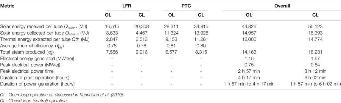
TABLE 8. Case study I: Performance of open-loop and closed control loop operation of HSTP.

7 Case Study II: Two Day Solar Radiation

The case study in previous section considered only a single day of operation with simulated solar radiation. In practise, the HSTP has to be started on a daily basis. The conditions during shutdown on the previous day will thus have a bearing on the current day operation. In this section, to further investigate the utility of the closed-loop operation vis-a-vis open-loop operation while considering this day-to-day operating requirement, we consider a 2-day operation scenario. The solar radiation used for this study is taken from 1 MWe Gurgaon plant on first May 2014 and the corresponding open-loop performance is discussed in literature (Kannaiyan et al., 2019). Startup strategy of HSTP is similar to that described in detail in our prior work (Kannaiyan et al., 2019). Shutdown condition is implemented as discussed in Section 6. Further, night time losses are also simulated in this case study to derive startup conditions on second day from the shutdown conditions on the first day (Kannaiyan et al., 2019).

Duration of HSTP plant operation and electric power generation on first day (cold startup) and second day (warm startup) along with CL operation and its performance compared with OL performance (dotted line) is shown in Figure 19. Table 9 shows the performance of OL and CL operation using various performance metrics. Similar to case study I, the utility of using decentralized plantwide control is evident in the significantly superior values of the metrics in the closed-loop when compared with open-loop operations. From Figure 19 it is seen that in CL operation, the electric power generation setpoint is tracked for much longer durations when compared to OL operation. In particular, on day two (warm startup), the generated power reaches and tracks the setpoint of 0.6 MWe from about 10.00 h onwards which is 2 hours after start of plant. In contrast, in OL operation, the setpoint is tracked only in late afternoon at about 15.00 h. Details of operating duration in OL and CL operation on both cold startup (day one) and hot startup (day two) operation and night time cooling duration is shown in Supplementary Table S6 in SI. During night time cooling, variation of thermal variables is shown in Supplementary Table S7 in SI.

FIGURE 19

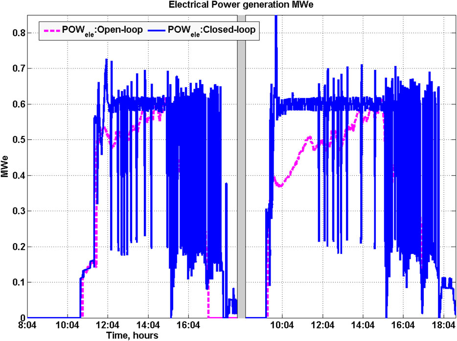
FIGURE 19. Case study II: Electric power profile of SG and SD in closed-loop and open-loop.

TABLE 9

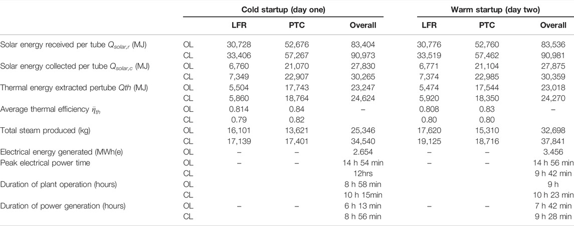
TABLE 9. Case study II: HSTP performance comparison OL and CL.

8 Conclusion

In this work, closed-loop control studies for the Hybrid Solar Thermal Power Plant (HSTP) were carried out. Using a dynamic simulator of the HSTP, step tests were performed to facilitate identification of control relevant models of various subsystems related to PTC, LFR, SG, and SD. Appropriate transfer functions were subsequently identified using the step-response data. Based on the identified transfer functions, PI and PID controllers were designed and implemented using IMC tuning rules. Apart from the feedback controllers, static feedforward controllers were also designed to compensate for various measured disturbances. Moreover, an override controller was also implemented for handling inventory constraints. The significance of the various elements of the control strategy was demonstrated using two case studies: a day-long dynamic simulation of the plant, using quadratic solar radiation with cloud cover, as well as a 2 day scenario with realistic solar radiation and considering night-time cooling effects. Plant performances of both closed and open-loop operations were compared. Results demonstrate the superior performance of the closed-loop operations on almost all metrics of relevance. In future, static feedforward control can be replaced by a dynamic feedforward control strategy along with use of decouplers to further improve controller performance. Subsequently, investigation of centralized control strategy, such as MPC can be undertaken. The performance achieved by the decentralized control strategy presented in the current work can then be used to benchmark the performances of these various strategies.

Data Availability Statement

The original contributions presented in the study are included in the article/Supplementary Material, further inquiries can be directed to the corresponding author.

Author Contributions

SK: Formal analysis, methodology, investigation, software, writing-original draft. SB: Conceptualization, supervision, methodology, writing-review editing. MB: Conceptualization, supervision, methodology, writing-review editing.

Conflict of Interest

The authors declare that the research was conducted in the absence of any commercial or financial relationships that could be construed as a potential conflict of interest.

Publisher’s Note

All claims expressed in this article are solely those of the authors and do not necessarily represent those of their affiliated organizations, or those of the publisher, the editors and the reviewers. Any product that may be evaluated in this article, or claim that may be made by its manufacturer, is not guaranteed or endorsed by the publisher.

Supplementary Material

The Supplementary Material for this article can be found online at: https://www.frontiersin.org/articles/10.3389/fcteg.2022.853625/full#supplementary-material

9 Appendix

The dynamic models of HSTP for various components are based on conservation principles. Dynamic equations formulation using first principle model of PTC, HXs, and HT/LT, LFR, and SD along with its Open-Loop (OL) simulation and its performance evaluation formulas are shown in detail in our prior work (Kannaiyan et al., 2019). In this section, we briefly summary the procedure for computing average thermal efficiency which has been listed in Tables 8 and 9.

9.1 Performance Evaluation

Average thermal efficiency of PTC and LFR fields used in case studies discussions are obtained as follows (Kannaiyan et al., 2019):

${\bar{\eta }}_{th}=\frac{Q_{th}}{Q_{\mathit{solar,c}}}(9)$

where

$Q_{th}=\left\{\begin{array}{c}\underset{Day}{\int }\left(q\left(t\right){|}_{x=L}{h}_{\left(st,o,LFR\right)}\left(t\right)+\left(1-q\left(t\right){|}_{x=L}\right)h_{\left(w,o,LFR\right)}\left(t\right)\right.\hfill \\ \left.-h_{\left(w,i,LFR\right)}\left(t\right)\right){\dot{m}}_{\left(w,i,LFR\right)}\left(t\right)dt,\hfill & \text{for\hspace{0.17em}LFR}\hfill \\ \underset{Day}{\int }\left(h_{\left(o,o,PTC\right)}\left(t\right)-h_{\left(o,i,PTC\right)}\left(t\right)\right){\dot{m}}_{\left(o,o,PTC\right)}\left(t\right)dt,\hfill & \text{for\hspace{0.17em}PTC}\hfill \end{array}\right.(10)$

is the total thermal energy extracted during the day long operation by the working fluid in the respective field. Further Q_solar,c is the daily solar energy collected by the respective fields which is computed as,

$Q_{\mathit{solar,c}}=\left\{\begin{array}{cc}{\eta }_{\left(opt,LFR\right)}{Q}_{\left(solar,r,LFR\right)}\hfill & \text{for\hspace{0.17em}LFR}\hfill \\ {\eta }_{\left(opt,PTC\right)}{Q}_{\left(solar,r,PTC\right)}\hfill & \text{for\hspace{0.17em}PTC}\hfill \end{array}\right.(11)$

with,

$Q_{\left(solar,r,LFR\right)}=\underset{Day}{\int }I\left(t\right)W_{\mathit{LFR}}{L}_{\mathit{LFR}}dt(12)$

$Q_{\left(solar,r,PTC\right)}=\underset{Day}{\int }I\left(t\right)W_{\mathit{PTC}}{L}_{\mathit{PTC}}dt(13)$

being the daily solar energy received by the respective fields. Note that η_(opt,LFR) = 0.22 and η_(opt,PTC) = 0.4 were considered for the case study.

References

Aurousseau, A., Vuillerme, V., and Bezian, J.-J. (2016). Control Systems for Direct Steam Generation in Linear Concentrating Solar Power Plants - A Review. Renew. Sustain. Energy Rev. 56, 611–630. doi:10.1016/j.rser.2015.11.083

CrossRef Full Text | Google Scholar

Barcia, L., Peón Menéndez, R., Martínez Esteban, J., José Prieto, M., Martín Ramos, J., de Cos Juez, F., et al. (2015). Dynamic Modeling of the Solar Field in Parabolic Trough Solar Power Plants. Energies 8, 13361–13377. doi:10.3390/en81212373

CrossRef Full Text | Google Scholar

Bequette, B. W. (2003). Process Control: Modeling, Design, and Simulation. Upper Saddle River, NJ: Prentice Hall.

Google Scholar

Camacho, E. F., and Berenguel, M. (1994). “Application of Generalized Predictive Control to a Solar Power Plant,” in The 1994 IEEE Conference on Control Applications. Part 3(of 3) Glasgow, UK. doi:10.1109/cca.1994.381468

CrossRef Full Text | Google Scholar

Camacho, E. F., and Gallego, A. J. (2013). Optimal Operation in Solar Trough Plants: A Case Study. Sol. Energy 95, 106–117. doi:10.1016/j.solener.2013.05.029

CrossRef Full Text | Google Scholar

Camacho, E. F., Rubio, F. R., Berenguel, M., and Valenzuela, L. (2007). A Survey on Control Schemes for Distributed Solar Collector Fields. Part I: Modeling and Basic Control Approaches. Sol. Energy 81, 1240–1251. doi:10.1016/j.solener.2007.01.002

CrossRef Full Text | Google Scholar

Camacho, E., Rubio, F., and Hughes, F. (1992). Self-tuning Control of a Solar Power Plant with a Distributed Collector Field. IEEE Control Syst. Mag. 12, 72–78. doi:10.1109/37.126858

CrossRef Full Text | Google Scholar

Desai, N. B., Bandyopadhyay, S., Nayak, J. K., Banerjee, R., and Kedare, S. B. (2014). Simulation of 1MWe Solar Thermal Power Plant. Energy Procedia 57, 507–516. doi:10.1016/j.egypro.2014.10.204

CrossRef Full Text | Google Scholar

Eck, M., and Hirsch, T. (2007). Dynamics and Control of Parabolic Trough Collector Loops with Direct Steam Generation. Sol. Energy 81, 268–279. doi:10.1016/j.solener.2006.01.008

CrossRef Full Text | Google Scholar

Gallego, A. J., and Camacho, E. F. (2012). Adaptative State-Space Model Predictive Control of a Parabolic-Trough Field. Control Eng. Pract. 20, 904–911. doi:10.1016/j.conengprac.2012.05.010

CrossRef Full Text | Google Scholar

Golder, A. K., and Goud, V. (2019). Condenser and Reboiler Design, National Programme on Technology Enhanced Learning (NPTEL). MoE, Govt of India. Available at: https://nptel.ac.in/courses/103103027 (Accessed June 9, 2022).

Google Scholar

Guo, S., Liu, D., Chen, X., Chu, Y., Xu, C., Liu, Q., et al. (2017). Model and Control Scheme for Recirculation Mode Direct Steam Generation Parabolic Trough Solar Power Plants. Appl. Energy 202, 700–714. doi:10.1016/j.apenergy.2017.05.127

CrossRef Full Text | Google Scholar

Johansen, T. A., Hunt, K. J., and Petersen, I. (2000). Gain-scheduled Control of a Solar Power Plant. Control Eng. Pract. 8, 1011–1022. doi:10.1016/s0967-0661(00)00043-5

CrossRef Full Text | Google Scholar

Kannaiyan, S., Bhartiya, S., and Bhushan, M. (2019). Dynamic Modeling and Simulation of a Hybrid Solar Thermal Power Plant. Ind. Eng. Chem. Res. 58, 7531–7550. doi:10.1021/acs.iecr.8b04730

CrossRef Full Text | Google Scholar

Kannaiyan, S., Bokde, N. D., and Geem, Z. W. (2020). Solar Collectors Modeling and Controller Design for Solar Thermal Power Plant. IEEE Access 8, 81425–81446. doi:10.1109/ACCESS.2020.2989003

CrossRef Full Text | Google Scholar

Li, X., Xu, E., Ma, L., Song, S., and Xu, L. (2019). Modeling and Dynamic Simulation of a Steam Generation System for a Parabolic Trough Solar Power Plant. Renew. Energy 132, 998–1017. doi:10.1016/j.renene.2018.06.094

CrossRef Full Text | Google Scholar

Nayak, J. K., Kedare, S. B., Banerjee, R., Bandyopadhyay, S., Desai, N. B., Paul, S., et al. (2015). A1 MW National Solar Thermal Research Cum Demonstration Facility at Gwalpahari, Haryana, India. Curr. Sci. 109, 1445–1457. doi:10.18520/v109/i8/1445-1457

CrossRef Full Text | Google Scholar

Nixon, J., Dey, P., and Davies, P. (2010). Which Is the Best Solar Thermal Collection Technology for Electricity Generation in North-West India? Evaluation of Options Using the Analytical Hierarchy Process. Energy 35, 5230–5240. doi:10.1016/j.energy.2010.07.042

CrossRef Full Text | Google Scholar

Rivera, D. E. (1999). Internal Model Control: A Comprehensive View. Tempe, Arizona: Arizona State University.

Google Scholar

Silva, R. N., Rato, L. M., and Lemos, J. M. (2003). Time Scaling Internal State Predictive Control of a Solar Plant. Control Eng. Pract. 11, 1459–1467. doi:10.1016/s0967-0661(03)00112-6

CrossRef Full Text | Google Scholar

Stephanopoulos, G. (1984). Chemical Process Control, 2. New Jersey: Prentice-Hall.

Google Scholar

Valenzuela, L., Zarza, E., Berenguel, M., and Camacho, E. F. (2005). Control Concepts for Direct Steam Generation in Parabolic Troughs. Sol. Energy 78, 301–311. doi:10.1016/j.solener.2004.05.008

CrossRef Full Text | Google Scholar

Wibowo, T. C. S., Saad, N., and Karsiti, M. N. (2009). “System Identification of an Interacting Series Process for Real-Time Model Predictive Control,” in 2009 American Control Conference (IEEE), 4384–4389. doi:10.1109/acc.2009.5160239

CrossRef Full Text | Google Scholar

Wittmann, M., Hirsch, T., and Eck, M. (2009). “Some Aspects of Parabolic Trough Field Operation with Oil as a Heat Transfer Fluid,” in 15th SolarPACES Symposium.

Google Scholar

Nomenclature

I Solar radiation (W/m²)

Pow_ele Electrical Power generated(MWe)

${\dot{m}}_{(o,i,PTC)}$ mass flow rate of oil flowing in towards PTC (kg/s)

${\dot{m}}_{(o,i,PTC),FF}$ mass flow rate of oil flowing in PTC from feedforward action (kg/s)

${\dot{m}}_{(w,i,LFR)}$ mass flow rate of water flow in towards LFR (kg/s)

${\dot{m}}_{(w,i,LFR),FF}$ mass flow rate of water flow in towards LFR from feedforward action (kg/s)

η_(opt,PTC) Optical efficiency of PTC

η_(opt,LFR) Optical efficiency of LFR

${\dot{m}}_{(o,i,HX)}$ mass flow rate of oil flow into HX (kg/s)

${\dot{m}}_{(w,i,HX)}$ mass flow rate of water flow into HX (kg/s)

he_(w, SD) height water present in SD (m)

${\dot{m}}_{(w,i,\mathrm{SD})}$ mass flow rate of water flow into SD (kg/s)

he_(w,SG) height water present in HX-SG(m)

${\dot{m}}_{(o,i,HT/LT)}$ mass flow rate of oil flow into HT/LT (kg/s)

${\dot{m}}_{(st,o,\mathrm{SD})}$ mass flow rate of steam out of SD (kg/s)

${\dot{m}}_{(2\varphi ,o,LFR)}$ mass flow rate of water/steam flow out of LFR(kg/s)

T_(o,i,HX) Temperature of oil flow into HX (^o C)

T_(w,i,HX) Temperature of water flow into HX (^o C)

T_(w,SG) Temperature of water present at SG (^o C)

T_(w,i, SD) Temperature of water flow into SD (^o C)

T_(w, SD) Temperature of water present at SD (^o C)

T_{(o,o,PTC−500m)} Temperature of oil flow out of PTC at 500 m (^o C)

T_(w,i,LFR) Temperature of water flow into LFR (^o C)

h_(o,i,HX) enthalpy of oil flow into HX (KJ/kg)

h_(o,o,HX) enthalpy of oil flow out of HX (KJ/kg)

h_(w,i,HX) enthalpy of water flow into HX (KJ/kg)

h_(w,o,HX) enthalpy of water flow out of HX (KJ/kg).