Integration of Photovoltaic Generation Within a Modeling Framework for Energy Hubs

Energy efficiency is a topic with many publications related to resource exploitation at a local scale; via well-performed energy management, substantial environmental and economic benefits can be achieved. In this article, the models used to forecast the photovoltaic power yield in two distinct facilities are described. These facilities are part of the same production plant, which makes use of different heterogeneous resources (carbon dioxide, water, thermal energy, and electricity) and has already been analyzed in a problem that consists in finding the set of variables that minimize the operation cost. In order to predict the power production for both photovoltaic fields, the expressions for radiation on sloped surfaces and the equivalent circuit for solar cells are employed, and the inverters and wire-transmission loss effects are considered. Furthermore, their integration within a general-purpose modeling framework for energy hubs is demonstrated. The comparison between validation results and production real data shows that despite the slight overestimation of the energy yield, the models are suitable to forecast the production of both facilities with a suitable accuracy, as the R² coefficients of both facilities lie between 0.95 and 0.96.

1 Introduction

The number of photovoltaic (PV) facilities in the world has significantly grown over the last decades, and they are expected to be a key piece in the future power system (Gul et al., 2016). According to Kazem and Yousif (2017), “PV applications have been employed in communications, crop irrigation, healthcare devices, lighting, water purification, environmental monitoring, cathode protection, air navigation and marine systems, utility power, and other commercial and residential applications.” However, despite the significant amount of energy hubs (EHs) where PV systems are included (Mohammadi et al., 2017), to the best of the author’s knowledge, most approaches consider just a fixed efficiency value for PV fields, and the possibility to regulate the power produced is often neglected; instead, it is assumed that the field yields as much power as the level of irradiance allows.

Whereas this can be acceptable for design applications, on other occasions, a better periodic estimate of the fields’ performance is required, for example, the cases of energy management strategies for self-consumers where the decisions hourly taken require forecast the power yield by a PV field (Ramos–Teodoro et al., 2018) or the design of facilities based on multilevel optimization (Evins 2015). In these cases, a static model for estimating the overall production from the actual weather conditions can be still enough for such purposes while keeping the computational burden low.

Consequently, the contributions of this article can be summarized as follows.

• Providing an example of integration of converters with time-variant coefficients within the modeling framework proposed by Ramos–Teodoro et al. (2018, 2020), whose main purpose is to be used for energy/resource management and dispatch problems.

• Validating a whole photovoltaic production model for two facilities with heterogeneous layout and data.

The remainder of this article is organized as follows: Section 2.1 introduces the building of the Solar Energy Research Center CIESOL and a PV parking located at the University of Almeria campus, which served as test-bed plants; Section 2.2 describes the modeling framework for which the PV generation model has been developed; Section 2.3 presents the main first principles models that have been well established in the literature for solar radiation on sloped surfaces and for PV (photovoltaic) cells, respectively, and details the arrangements made to consider the inversion and transmission losses in the PV (photovoltaic) facilities, including curve fitting for some of the parameters; Section 3 real data are employed to test the validity of the parameters characterized in the previous sections; and Section 4 synthesizes the authors’ reflections and elucidates possible future enhancements for the production model described in the following text.

2 Materials and Methods

2.1 CIESOL Building and Photovoltaic Parking

The Solar Energy Research Center (CIESOL) was founded in 2005, thanks to an agreement between the University of Almeria and the Center for Energy, Environment, and Technology (CIEMAT) of the Ministry of Economy and Competitiveness. The center is located at the University of Almeria campus (36.83°N, 2.41°W), in a building which receives the same name as the center: The CIESOL building (Figure 1). This has a total surface area of 1071.92 m², laid out on two floors, and was built following bioclimatic criteria, incorporating several energy-saving passive and active strategies. A vast network of sensors allows recording and monitoring information in order to determine, or at least estimate with a high degree of confidence, CIESOL’s energy consumption, outdoor and indoor climate conditions, and occupancy, among others.

FIGURE 1

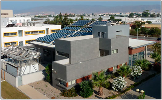
FIGURE 1. Backside picture of the CIESOL building where the photovoltaic field and the field of solar collectors are visible in the rooftop.

Although the main facilities of interest and their features are summarized in the following text, readers are referred to Castilla et al.’s book which contains a detailed description of CIESOL (Castilla et al., 2014). The PV field is composed of forty-two Atersa A-222P modules, facing south (azimuthal angle of 21° east), with a surface area of 1,63 m² and a slope angle of 22°, and distributed in three arrays of fourteen collectors each, connected in series (seven on the left and seven on the right at the highest part of the roof, as shown in Figure 1). Each array feeds a CICLO-3000 inverter where the electrical parameters related to production are measured and sent to a database, mainly direct current and voltage as well as alternate current and voltage at each inverter.

On the other hand, the PV parking of the University of Almeria (36.83°N, 2.40°W), shown in Figure 2, consists of ten arrays of 483 Conergy PA 240P modules (twenty-one in series and twenty-three in parallel) connected to a Fronius Agilo 100 inverter (4,830 modules and ten inverters in total) for production purposes, as well as another three arrays for experimental testing, connected to their respective Fronius IG Plus 55v3 inverters, and distributed as follows: twenty-four Conergy PA 240P modules (twelve in series and two in parallel) in the first group, twenty-four Conergy Power Plus 240M modules (twelve in series and two in parallel) in the second, and seventy-two First Solar FS-380 modules (eight in series and nine in parallel) in the third. All the modules have a slope angle of 7° and are facing south (azimuthal angle of 21° east).

FIGURE 2

FIGURE 2. Photovoltaic parking at the University of Almeria.

2.2 Prior Modeling Framework for Energy Hubs

In broad terms, the models of most EHs represent energy and mass balances between a set of input resources that can be transformed into another set of output resources. These resources are represented mathematically through variables which constitute the, respective, input and output vector elements. The basic relationship proposed by Geidl and Andersson (2007) is based on a coupling matrix C that represents the conversion process between multiple energy carriers in the steady state (L − CP = 0), where P is the input power or source and L is the output power or load. The coefficients of this matrix are given by the product of the efficiencies of all the conversion units or devices that intervene in the conversion and the so-called dispatch factors that need to be introduced whenever one energy carrier splits up to several flows inside the EH. Additional constraints may consider power limits, the presence of storage systems, and necessary energy balances among these dispatch factors.

This has led to formulations that have progressively introduced elements to represent conversion and storage processes more accurately but share a similar basis. In contrast to other proposals in the literature, the model developed by the authors of this article defines a “path vector” whose elements are decision variables for each possible path between inputs and outputs. This allows avoiding the nonlinear relationships of Geidl and Andersson’s model when two dispatch factors are multiplied in the coupling matrix, and to formulate the conversion model of complex EHs in a simpler manner, with fewer decision variables. The input and internal flows are obtained from the elements of the path vector and suitably defined coupling matrices. Some outputs or loads can be considered dependent on the fact that certain device is turned on or off, which was taken into account in the model by arranging Geidl and Andersson’s equation L − CP = 0. Readers are referred to the articles published by Ramos–Teodoro et al. (2018, 2020) for further information on the full model of which some equations are presented in the following text.

2.2.1 Conversion Model

Considering the most common elements in previous approaches, the conversion and storage model of a general EH needs a minimum set of variables representing the structure of the system to be defined. Therefore, let N_i represent the number of input flows, N_o the number of output flows, N_p the number of paths between these inputs and outputs, N_d the number of conversion devices with a total amount of N_di input flows, and N_do output flows. Also, the equations are represented in discrete time, with a uniform sample time T = t(k + 1) − t(k), where k constitutes any discrete-time instant. Thus, the conversion processes need to satisfy the balance conditions at each time step, as stated in Eq. 1,

${\mathit{\delta }}_{\mathit{O}}\left(k\right)\mathit{O}\left(k\right)+\mathit{M}\left(k\right)=\mathit{C}\left(k\right)\mathit{P}\left(k\right)-{\mathit{Q}}_{\mathit{c}\mathit{h}}\left(k\right)+{\mathit{Q}}_{\mathit{d}\mathit{i}\mathit{s}}\left(k\right),(1)$

where P is the N_p × 1 vector of flows between inputs and outputs or “path vector,” M is the N_o × 1 vector of market sales flows, O is the N_o × 1 vector of output flows, Q_ch is the N_o × 1 vector of charge flows, Q_dis is the N_o × 1 vector of discharge flows, C is the N_o × N_p coupling matrix, and δ_O is the N_o × N_o binary diagonal matrix of output activation.

Additionally, the relationship between the internal P vector flows and both the input flows to the EH itself must be established, as defined in Eq. 2, and the input–output flows in each device, as given in Eqs 3, 4.

$\mathit{I}\left(k\right)={\mathit{C}}_{\mathit{i}}\mathit{P}\left(k\right),(2)$

${\mathit{D}}_{\mathit{i}}\left(k\right)={\mathit{C}}_{\mathit{d}\mathit{i}}\left(k\right)\mathit{P}\left(k\right),(3)$

${\mathit{D}}_{\mathit{o}}\left(k\right)={\mathit{C}}_{\mathit{d}\mathit{o}}\left(k\right)\mathit{P}\left(k\right),(4)$

where I is the N_i × 1 vector of input flows, D_i is the N_di × 1 vector of devices’ flows (referred to their inputs), D_o is the N_do × 1 vector of devices’ flows (referred to their outputs), C_i is the N_i × N_p input coupling matrix, C_di is the N_di × N_p device coupling matrix (referred to their inputs), and C_do is the N_do × N_p device coupling matrix (referred to their outputs).

Except vector O, which a priori does not contain decision variables, and vector P, which is indirectly limited by the production capacity of the conversion devices from the following equations, the remaining vectors need to be constrained in order to ensure that the conversion devices do not exceed their defined capacities. That is the raison d’être of Eqs 5–8,

${\mathit{M}}^{\mathit{min}}\left(k\right){\mathit{\delta }}_{\mathit{M}}\left(k\right)\le \mathit{M}\left(k\right)\le {\mathit{M}}^{\mathit{max}}\left(k\right){\mathit{\delta }}_{\mathit{M}}\left(k\right),(5)$

${\mathit{I}}^{\mathit{min}}\left(k\right){\mathit{\delta }}_{\mathit{I}}\left(k\right)\le \mathit{I}\left(k\right)\le {\mathit{I}}^{\mathit{max}}\left(k\right){\mathit{\delta }}_{\mathit{I}}\left(k\right),(6)$

${\mathit{D}}_{\mathit{i}}^{\mathit{min}}\left(k\right){\mathit{\delta }}_{{\mathit{D}}_{\mathit{i}}}\left(k\right)\le {\mathit{D}}_{\mathit{i}}\left(k\right)\le {\mathit{D}}_{\mathit{i}}^{\mathit{max}}\left(k\right){\mathit{\delta }}_{{\mathit{D}}_{\mathit{i}}}\left(k\right),(7)$

${\mathit{D}}_{\mathit{o}}^{\mathit{min}}\left(k\right){\mathit{\delta }}_{{\mathit{D}}_{\mathit{o}}}\left(k\right)\le {\mathit{D}}_{\mathit{o}}\left(k\right)\le {\mathit{D}}_{\mathit{o}}^{\mathit{max}}\left(k\right){\mathit{\delta }}_{{\mathit{D}}_{\mathit{o}}}\left(k\right),(8)$

where the superscripts “max” and “min” refer to the upper or lower limits of each vector, respectively (e.g., I^max determines the maximum amount of resources that can enter the EH), and the rest of δ symbols define diagonal binary variables that indicate if the flow is allowed or not. In particular, δ_M is the N_o × N_o binary diagonal matrix of market sales flow activation, δ_I is the N_i × N_i binary diagonal matrix of input flow activation, ${\mathit{\delta }}_{{\mathit{D}}_{\mathit{i}}}$ is the N_di × N_di binary diagonal matrix of devices’ flow activation (referred to their inputs), and ${\mathit{\delta }}_{{\mathit{D}}_{\mathit{o}}}$ is the N_do × N_do binary diagonal matrix of devices’ flow activation (referred to their outputs).

2.2.2 Conversion and Capacity Models

The element of the vectors that bound the flows within the energy hub (denoted with the superscripts “max” and “min”) and of the coupling matrices that contain values of efficiencies (denoted with the letter “C”) are defined in coherence with the physical component that they represent. Most values in the above matrices and vectors are defined by setting the lower bound to zero and the upper bound to infinite for unconstrained flows, and setting the efficiencies to zero (instead of minus infinite, which would lead to having undesirable reverse flows) when there is no possible flow among devices/EHs or to one in lossless conversion/transportation processes. Many other processes occurring in the EH are actually characterized as having complex dynamics which cannot be entirely reflected in the above equations without these being reformulated, affecting how the former parameters are defined.

Such issues have already been tackled, for example, by Evins et al., who proposed methods to prevent devices from starting up too frequently and to turn the nonlinear dynamic of load-dependent efficiencies into step-wise curves (Evins et al., 2014). In order to keep things simple, the usual approach of the authors of this article lies in using constants, usually from manufacturers’ specifications and considering that they cover the main range of operation of each device; or time-variant coefficients, which should be deductible from the models that dictate the behavior of each process. The latter is the reason why the parameters of the model presented by them depend on k (Ramos–Teodoro et al., 2018, 2020), which is relevant to facilities such as PV fields, whose production along the day needs to be calculated with the models presented in the following sections.

2.3 Solar PV Generation Forecasting

2.3.1 Time-Variant Coefficients for PV Facilities

Considering a uniform sample time T = t(k + 1) − t(k), where k constitutes any discrete time instant, as previously defined, the relationship among the incident radiation on an array of PV modules, the amount of DC (direct current) power produced by them, and the one supplied to the AC (alternating current) grid can be obtained by arranging Eq. (23.7.1) from Duffie and Beckman’s book into Eq. 9:

$P_{c,ac}\left(k\right)=G_T\left(k\right)A_c{\eta }_{c,mpp}\left(k\right){\eta }_{c,inv}\left(k\right){\eta }_{c,ac},(9)$

where P_c,ac is the amount of AC power supplied to the grid by the array, G_T is the incident solar irradiance on the (tilted) surface of array c (see Section 2.3.2 for calculations), A_c is the total area of array c (see Section 2.3.3 for technical information), η_c,mpp is the maximum power point efficiency of array c (see Section 2.3.3 for calculations), η_c,inv is the efficiency of the inverter connected to array c (see Section 2.4 for calculations), and η_c,ac is the transmission efficiency from the inverter to the point of supply of array c (see Section 2.4 for calculations).

The following sections describe the way these parameters would be computed in the previous modeling framework, and, once their value is known, how they are introduced as constraints, as stated in Eqs 10, 11 for a device D_pv representing the entire PV field with a set $\mathcal{F}$ of N_c arrays,

$D_{i,pv}^{\max }\left(k\right)=G_T\left(k\right)\sum _{c\in \mathcal{F}}{A}_c,(10)$

$C_{pv}\left(k\right)=\sum _{c\in \mathcal{F}}\frac{{\eta }_{c,mpp}\left(k\right){\eta }_{c,inv}\left(k\right){\eta }_{c,ac}}{N_c},(11)$

where $D_{i,pv}^{\max }$ is the upper limit of the flow (solar radiation) entering the device (field) which will be an element of the ${\mathit{D}}_{\mathit{i}}^{\mathit{max}}$ vector, and C_pv is the gross efficiency of the field which will be an element of the coupling matrices presented earlier.

2.3.2 Solar Irradiance on Sloped Surfaces

Although both the anisotropic and the isotropic sky models have been implemented, the validation and the case study presented in this article were carried out only using the second one, which is described in the following text based on the explanations found in Duffie and Beckman’s book (Duffie and Beckman, 2013). First, the total solar irradiance on a tilted surface is given by Eq. 12,

$G_T\left(k\right)=G_b\left(k\right)R_b\left(k\right)+G_d\left(k\right)\frac{1+\cos \beta }{2}+G\left(k\right){\rho }_g\frac{1-\cos \beta }{2},(12)$

where G_b is the BHI (beam horizontal irradiance), G_d is the DHI (diffuse horizontal irradiance), G is the GHI (global horizontal irradiance), that is, the sum of G_b(k) and G_d(k), R_b is the ratio of beam radiation on a tilted plane to that on the plane of measurement (usually horizontal), ρ_g is the ground reflectance (assumed to be of 0.1), and β is the slope angle of the modules.

To forecast the production, it is necessary to know the three terms of the irradiance on the horizontal plane, which in practice can be provided by organizations such as the Spanish National Weather Agency AEMET. For the validation presented in this section, the historical data recorded by the CIESOL’s weather station were used instead. In either case, the beam irradiance tends to be indirectly determined from the DNI (direct normal irradiance) on the horizontal plane (or direct beam irradiance), which is the magnitude actually measured by the pyrheliometers. Their relationship is given by Eq. 13,

$G_b\left(k\right)=G_{bn}\left(k\right)\cos {\theta }_z,(13)$

where G_bn is the DNI (direct normal irradiance) and θ_z is the zenith angle.

Except ρ_g(k) and the irradiances, the rest of the variables appearing in Eq. 12 are geometrical parameters to be taken into account for determining the position of the Sun in the sky, which are related by means of Eqs 14, 15, and 16,

$R_b\left(k\right)=\frac{\cos \theta \left(k\right)}{\cos {\theta }_z\left(k\right)},(14)$

$\begin{array}{cc}\hfill \cos \theta \left(k\right)=& \sin \delta \left(k\right)\sin \varphi \cos \beta -\sin \delta \left(k\right)\cos \varphi \sin \beta \cos \gamma +\cos \delta \left(k\right)\cos \varphi \cos \beta \cos \omega \left(k\right)\hfill \\ \hfill & +\cos \delta \left(k\right)\sin \varphi \sin \beta \cos \gamma \cos \omega \left(k\right)+\cos \delta \left(k\right)\sin \beta \sin \gamma \sin \omega \left(k\right),\hfill \end{array}(15)$

$\cos {\theta }_z\left(k\right)=\sin \delta \left(k\right)\sin \varphi +\cos \delta \left(k\right)\cos \varphi \cos \omega \left(k\right),(16)$

where θ is the angle of incidence, γ is the surface azimuth angle or deviation between the orientation of the field and the south (east negative and west positive), ϕ is the latitude where the field is located (south negative and north positive), δ is the declination of the Sun, which measures the displacement of the Sun due to translation of the earth, and ω is the hour angle, which measures the displacement of the Sun due to rotation of the earth. Note that Eq. 16 corresponds to Eq. 15 particularized for β = 0°, that is, a horizontal surface.

Most of the previously mentioned parameters depend on the design of the field and are constants since these fields are supposed to be static (without solar tracking), but the remaining Eqs 17–21 provide the way to calculate them from ordinary variables such as time and day,

$\delta \left(k\right)=23.45\sin \left(360\frac{284+DoY\left(k\right)}{n_{days}\left(k\right)}\right),(17)$

$\omega \left(k\right)=360\frac{h_s\left(k\right)-12}{24},(18)$

$h_s\left(k\right)=h_o\left(k\right)+\frac{24}{360}\left({\psi }_{ref}-\psi \right)+\frac{1}{3600}EoT\left(k\right)-DST\left(k\right),(19)$

$\begin{array}{cc}\hfill EoT\left(k\right)=13.752\left(\right.0.075& +1.868\cos B\left(k\right)-32.077\sin B\left(k\right)\hfill \\ \hfill & -14.615\cos 2B\left(k\right)-40.89\sin 2B\left(k\right)\left.\right)),\hfill \end{array}(20)$

$B\left(k\right)=\left(1-DoY\left(k\right)\right)360/n_{days}\left(k\right),(21)$

where DoY is the day of the year (from 1 to 365 or 366), n_days is the total number of days of the year (365 or 366, depending on if it is a leap year or not), h_s is the solar time (expressed in hours), h_o is the official time (expressed in hours), ψ is the longitude where the field is located (from 0 to 360° west), ψ_ref is the longitude of the standard meridian for the local time zone (from 0 to 360° west), EoT is the result of evaluating the so-called equation of time (expressed in seconds), DST is the offset due to daylight saving time (expressed in hours), and B is the relative day for the equation of time.

In above and the following equations, when sunrise (or sunset) occurs at time k or nearly that time, the cosine of θ_z will tend zero and therefore, R_b will take very large values that tend to infinite (Duffie and Beckman, 2013). Since they are employed to obtain the integrated production between two time steps (usually 1-h intervals), the procedure to avoid that problem consists in calculating the above variables for the midpoint of each interval, which in such cases must range from the sunrise to the end of the time step (or from the start of the time step to the sunset), similar as TRNSYS software does (Klein et al., 2017). On the other hand, the parameters of the fields employed in the validation are recapped in Table 1 from Section 2.1.

TABLE 1

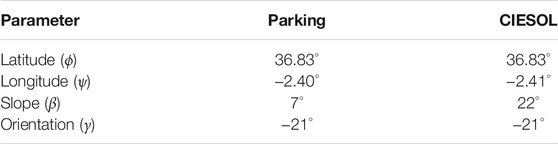
TABLE 1. Location and geometry of the PV fields.

2.3.3 Equivalent Circuit for Photovoltaic Cells

The model of the equivalent circuit for PV cells “can be used for an individual cell, a module consisting of several cells, or an array consisting of several modules” (Duffie and Beckman, 2013), and it is easy to apply because the parameters required can be deduced from the ones given by the manufacturers at standard conditions (G_st = 1000 W/m², T_m,st = 25°C). Considering the four types of PV modules described in Section 2.1, Atersa A-222P (M1), Conergy PA 240P (M2), Conergy Power Plus 240M (M3), and First Solar FS-380 (M4), the characteristics from their datasheet required to fit the model are presented in Table 2.

TABLE 2

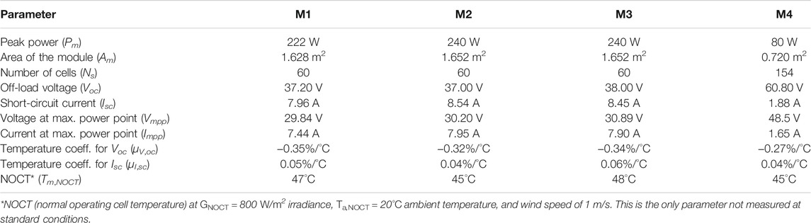
TABLE 2. Technical characteristics of the PV modules at standard conditions.

On the other hand, the model of the equivalent circuit is given by the five parameters shown in Eq. 22, from which the I − V curve can be obtained,

$I\left(k\right)=I_L\left(k\right)-I_o\left(k\right)\left[e^{\left(\frac{V\left(k\right)+I\left(k\right)R_s\left(k\right)}{a\left(k\right)}\right)}-1\right]-\frac{V\left(k\right)+I\left(k\right)R_s\left(k\right)}{R_{sh}\left(k\right)},(22)$

where I_L is the light current, I_o is the diode reverse saturation current, R_s is the series resistance, R_sh is the shunt resistance, a is the modified ideality factor of the diode, I is the current generated by the module, and V is the voltage of the module. However, Eq. 22 is not valid for any situation, but its parameters need to be updated according to the operating conditions and the technical characteristics of the PV modules. Duffie and Beckman described the procedure to do so, although this is not reproduced here because Simulink^® and its PV Array block were used instead to transform Table 2 into Table 3, which contains the five parameters at reference conditions (in this case, the standard conditions at which the manufacturer made the measurements of Table 2). Note that a_st is not obtained directly but by means of Eq. 23, according to the definition of the parameter that the authors give (Duffie and Beckman, 2013),

$a_{st}=k_B{n}_d{T}_{m,st}{N}_s/q,(23)$

where k_B is the Boltzmann constant (1.381 ⋅ 10⁻²³ J/K), n_d is the ideality factor of the diode (as provided by PV Array), T_m,st is the temperature of the module at standard conditions (25°C), N_s is the number of cells of the module (see Table 2), and q is the electronic charge (1.602 ⋅ 10⁻¹⁹ C).

TABLE 3

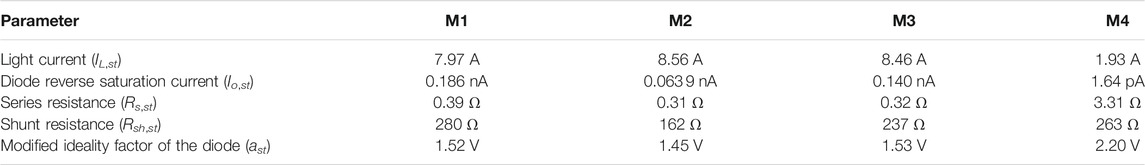
TABLE 3. Parameters of the equivalent circuit at standard conditions for the PV modules.

From Table 3, the five parameters of Eq. 22 can be updated at each time step, considering the relationships given by Eqs 24–29,

$\frac{a\left(k\right)}{a_{st}}=\frac{T_m\left(k\right)+273}{T_{m,st}+273},(24)$

$I_L\left(k\right)=\frac{S_T\left(k\right)}{S_{T,st}}\left[I_{L,st}+{\mu }_{I,sc}\left(T_m\left(k\right)-T_{m,st}\right)\right],(25)$

$\frac{I_o\left(k\right)}{I_{o,st}}={\left(\frac{T_m\left(k\right)+273}{T_{m,st}+273}\right)}^3{e}^{\left(f_{eV}\frac{E_{g,st}}{k_B\left(T_{m,st}+273\right)}-f_{eV}\frac{E_g\left(k\right)}{k_B\left(T_c\left(k\right)+273\right)}\right)},(26)$

$\frac{E_g\left(k\right)}{E_{g,st}}=1-C_{T,Eg}\left(T_m\left(k\right)-T_{m,st}\right),(27)$

$\frac{R_{sh}\left(k\right)}{R_{sh,st}}=\frac{S_{T,st}}{S_T\left(k\right)},(28)$

$R_s\left(k\right)=R_{s,st},(29)$

where T_m is the temperature of the module, T_m,st is the temperature of the module at standard conditions, E_g is the material bandgap energy, E_g,st is the material bandgap energy at standard conditions (1.12 eV for silicon), f_eV is the conversion factor from electron-volts to joules (1.602 ⋅ 10⁻¹⁹ J/eV), C_T,Eg is a fitting coefficient (0,0002677°C⁻¹ for silicon) (Duffie and Beckman, 2013), S_T is the effective irradiance absorbed by the module, and S_T,st is the effective irradiance absorbed by the module at standard conditions. Note that temperatures must be introduced in Kelvin in Eqs 24, 26 and that according to Table 2, μ_I,sc must to be multiplied by I_sc and divided by 100 in order to be transformed from percentage to absolute value (which some manufacturers provide too).

Regarding the last two parameters that would be required to determine the above equations, the effective absorbed solar ratio (S_T(k)/S_T,st) is estimated by applying Fresnel’s equations and Snell’s law, as well as rearranging Eq. 12 to consider the effect of the air mass, the incidence angle, and the spectroscopic behavior of the materials. Readers are referred to Chapter 5 in Duffie and Beckman’s book for further information, but most of the parameters involved have been presented in Section 2.3.2 and the new ones required are related to the cover of the modules, which is made of glass. A glazing thickness of 3.2 mm, a glazing extinction coefficient of 4 m⁻¹, and an air-glass refractive index of 1.526 were considered in all cases.

On the other hand, the module temperature is calculated from Eq. 30,

$T_m\left(k\right)=T_a\left(k\right)+\left(T_{m,NOCT}-T_{a,NOCT}\right)\frac{G_T\left(k\right)}{G_{NOCT}}\left(1-\frac{{\eta }_{c,mpp}\left(k\right)}{0.9}\right),(30)$

where T_a is the ambient temperature, and the remaining parameters have been defined previously (see Table 2 for NOCT conditions). As the efficiency appears in this equation (all the modules forming an array are considered to have the same efficiency), the temperature of the module is obtained by iteratively computing the equations presented in this section from an initial guess of η_c,mpp = 0.12 and with a termination criterion based on the change of the efficiency, which must be less than 0.001 in two consecutive steps to force convergence—“since the module efficiency is not a strong function of temperature, the process will converge rapidly” (Duffie and Beckman, 2013). Each new value is obtained assuming that the maximum power point is being tracked in the facilities and neglecting the effect of the wind on the module temperature in Eq. 30. As demonstrated by Duffie and Beckman 2013, differentiating Eq. 22 with respect to V and setting the result equal to zero leads to Eq. 31,

$\frac{I_{mpp}\left(k\right)}{V_{mpp}\left(k\right)}=\frac{\frac{I_o\left(k\right)}{a\left(k\right)}{e}^{\left(\frac{V_{mpp}\left(k\right)+I_{mpp}\left(k\right)R_s\left(k\right)}{a\left(k\right)}\right)}+\frac{1}{R_{sh}\left(k\right)}}{1+\frac{R_s\left(k\right)}{R_{sh}\left(k\right)}+\frac{I_o\left(k\right)R_s\left(k\right)}{a\left(k\right)}{e}^{\left(\frac{V_{mpp}\left(k\right)+I_{mpp}\left(k\right)R_s\left(k\right)}{a\left(k\right)}\right)}},(31)$

where I_mpp is the current generated by the module at maximum power point, and V_mpp is the voltage of the module at maximum power point; and, on the other hand, Eq. 22 needs to be satisfied at the same point, which results in Eq. 32,

$I_{mpp}\left(k\right)=I_L\left(k\right)-I_o\left(k\right)\left[e^{\left(\frac{V_{mpp}\left(k\right)+I_{mpp}\left(k\right)R_s\left(k\right)}{a\left(k\right)}\right)}-1\right]-\frac{V_{mpp}\left(k\right)+I_{mpp}\left(k\right)R_s\left(k\right)}{R_{sh}\left(k\right)}.(32)$

The simultaneous solution of both equations allows determining the maximum power point current and voltage, and therefore the efficiency of the array, as concluded in Eq. 33,

${\eta }_{c,mpp}\left(k\right)=\frac{V_{mpp}\left(k\right)I_{mpp}\left(k\right)}{G_T\left(k\right)A_m\left(k\right)1000}.(33)$

2.4 Inversion and Transmission Losses

Owing to the heterogeneity of the available data and the differences found in the two facilities under study, the methods to calculate the inversion and transmission losses in this section rather provide a rough estimate of them, which for the purpose of the developed models will be enough.

On the one hand, CIESOL’s dataset consists of minutely data from October 2013 to April 2017 of the inverters’ electrical measurements (direct and alternating current, voltage, and power) so that no transmission losses are considered because they are located very close to the PV field (η_c,ac = 1 for all the CIESOL’s arrays). The inconvenience is that the manufacturer of those CICLO-3000 inverters does not offer information on their efficiency, and therefore, they need to be determined from the abovementioned measurements. Figure 3 shows the exponential curves fitted to the data of the three inverters, where some isolated samples and the ones corresponding to efficiencies greater than one have been eliminated, especially in the inverters 1 and 3. Despite being identical devices and arrays, the curves’ parameters differ from each other, and although the correlation coefficients (R²) are close to one, a more in-depth analysis would be advisable, probably including additional variables such as the DC voltage (multiple regression), to improve these results. The main inconvenience would be that this equipment cannot be studied under laboratory conditions because it is a part of the building’s power supply system. Considering the actual results, the efficiency of each inverter is computed in Eq. 11 after obtaining the amount of power produced by the array to which they are connected (P_c,dc) and substituting that value in the corresponding exponential curve (see Figure 3).

FIGURE 3

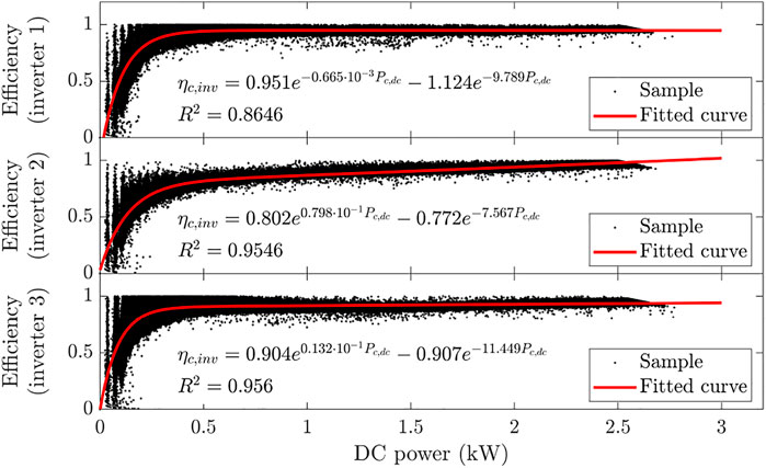
FIGURE 3. Curve fitting for the inverters of CIESOL’s PV field.

On the other hand, the dataset of the parking only contains the gross daily power produced from January 2013 to March 2014, measured by the general electric meter, and the monthly production of this one and the inverters; hence, there is no way to certainly know any of the electrical variables related to neither the inverters nor the fields, required to better fit the model. Instead, the efficiency curves of the manufacturer are considered for each kind of inverter (Fronius Agilo 100 and Fronius IG+ 55v3, see Section 2), summarized in Table 4, and the transmission losses are approximated by means of a simple linear regression between the two monthly measurements, which leads to an efficiency of η_c,ac = 0.978 for all the parking’s arrays (see Figure 4).

TABLE 4

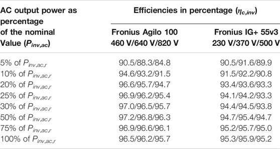
TABLE 4. Efficiencies of the parking’s inverters as a function of the DC input voltage (minimum, nominal, and maximum) and the AC output power, according to the manufacturer’s datasheet.

FIGURE 4

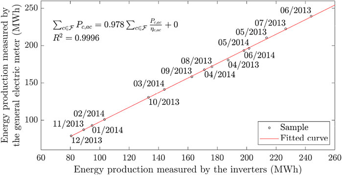
FIGURE 4. Curve fitting for the transmission losses of the parking’s PV field.

Since the arrays consist of modules of the same type, and neglecting any transmission loss occurring between the modules and the inverter’s input, in each case, the DC input voltage (V_c,dc) and power (P_c,dc) to the inverter can be obtained considering the fundamentals of Section 2.3.3, as expressed in Eqs 34, 35.

$V_{c,dc}\left(k\right)=V_{mpp}\left(k\right)N_{se},(34)$

$P_{c,dc}\left(k\right)=V_{mpp}\left(k\right)I_{mpp}\left(k\right)N_{se}{N}_{pa}/1000,(35)$

where N_se is the number of modules connected in series, and N_pa is the number of modules connected in parallel. Note that curves in Figure 3 directly provide the value of the inverter’s efficiency at each k, but, for the parking, several operations need to be carried out on the values of Table 4, as explained in the following text.

• First, column 1 is expressed in terms of absolute values (instead of percentages of P_inv,ac,r) for each type of inverter, considering the AC nominal output powers given in Table 5.

• Second, for each voltage, and given the efficiencies of Table 4, it is possible to calculate the equivalent DC input power that would replace the values of column 1 by applying P_c,dc = P_inv,ac/η_c,inv.

• Third, from a double linear interpolation of the values yielded by Eqs 34, 35, the actual efficiency of the inverter is obtained at each k.

TABLE 5

TABLE 5. DC nominal input power and AC nominal output power of the parking’s inverters, according to the manufacturer’s datasheet.

3 Results

In order to validate the previously presented model, different approaches were considered for CIESOL and the parking. In the first case, the daily ME (mean error), NRMSE (normalized root-mean-square error), and the coefficient of determination R² were calculated for the estimation of the generated power at a 1-min resolution, and normalized by the difference of the maximum and minimum values of the data, as stated in Eqs 36, 37, and 38.

$ME=\sum _{j=1}^{1440}\sum _{c\in \mathcal{F}}\frac{P_{c,ac}\left(j\right)-{\widehat{P}}_{c,ac}\left(j\right)}{1440},(36)$

$NRMSE=\frac{\sqrt{{\sum }_{j=1}^{1440}{\sum }_{c\in \mathcal{F}}\frac{{\left(P_{c,ac}\left(j\right)-{\widehat{P}}_{c,ac}\left(j\right)\right)}^2}{1440}}}{\max \left(P_{c,ac}\left(j\right)\right)-\min \left(P_{c,ac}\left(j\right)\right)},(37)$

$R^2=1-\frac{{\sum }_{j=1}^{1440}{\sum }_{c\in \mathcal{F}}{\left(P_{c,ac}\left(j\right)-{\widehat{P}}_{c,ac}\left(j\right)\right)}^2}{{\left(P_{c,ac}\left(j\right)-{\sum }_{j=1}^{1440}{\sum }_{c\in \mathcal{F}}{P}_{c,ac}\left(j\right)/1440\right)}^2},(38)$

whereP_c,ac(j) is the AC power produced by array c at min j, and ${\widehat{P}}_{c,ac}(j)$ is the estimate of the AC power produced by array c at min j. Figure 5 shows a bar diagram containing the distribution of these indices over the period of time analyzed, where the gaps between data correspond to missing or inconsistent samples (mainly unfeasible power values or incomplete records due to electrical outages, maintenance operations, or sensor failures). They are especially noticeable in the NRMSE because its value is always greater than 1.51, as summarized in Table 6, and therefore, those gaps are easily identified by the absence of bars. Readers are referred to Ramos–Teodoro et al.’s (2021) work for further information on the data cleansing performed in this study.

FIGURE 5

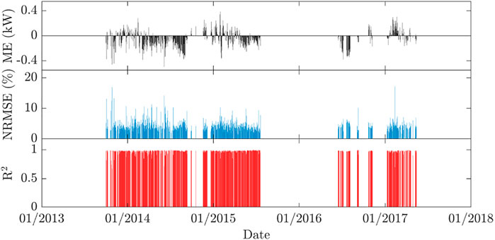
FIGURE 5. Distribution of the ME, NRMSE, and R² from the data available for CIESOL.

TABLE 6

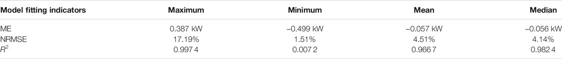
TABLE 6. Reference values of the ME and the NRMSE for the fitted model (CIESOL).

In order to give a further idea of the fitting, Figure 6 presents both the worst and the best performing predictions for CIESOL in terms of absolute NRMSE 1) and considering the same index but, as an additional condition to examine the performance with clear sky, only among the days in which the mean power generated is greater than 4 kW 2); and in Figure 7, the ordinary and cumulative probability distribution histograms (i.e., the frequencies of observations divided by the total number of samples) are also shown for the 1-min data. Note that the mean value of the ME is negative in the abovementioned results, which implies that the model tends to slightly overestimate the production. The probability distribution histograms in Figure 7, constructed from 450948 samples and 672 intervals, also support these claims and show an approximate symmetry of the error’s distribution with respect to the mean value.

FIGURE 6

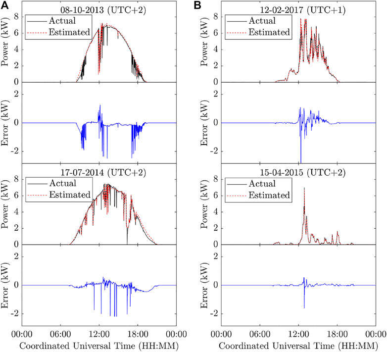
FIGURE 6. Worst (top) and best (bottom) validation for CIESOL’s PV field in different days. The days were selected according to the absolute value of the NRMSE (A) and considering the same index but as an additional condition to examine the performance with clear sky, only among the days in which the mean power generated is greater than 4 kW (B).

FIGURE 7

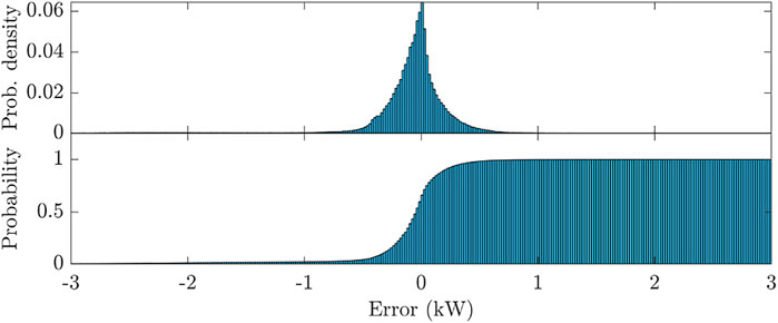
FIGURE 7. Ordinary and cumulative probability distribution histograms of the 1-min error for CIESOL’s PV field.

On the other hand, the results for the parking are encapsulated in Figure 8, which presents both the validation and the values of the indices defined previously, which have been calculated for the whole period of data by changing the units and the amount of samples in Eqs 36, 37, and 38, that is, using MWh instead of kW and replacing 1,440 (the number of minutes in a day) by 292 (the number of days with consistent data). In comparison to CIESOL, the results are not hopeless because the model still provides a good estimate of the energy yield (see the 0.9524 coefficient of determination and the 5.6% NRMSE), although the mean error is again negative but significantly higher. The probability distribution histograms in Figure 9, constructed from 292 samples and 17 intervals, also reflect this deviation from the ideal zero mean value and shows again an approximate symmetry of the error’s distribution with respect to this one.

FIGURE 8

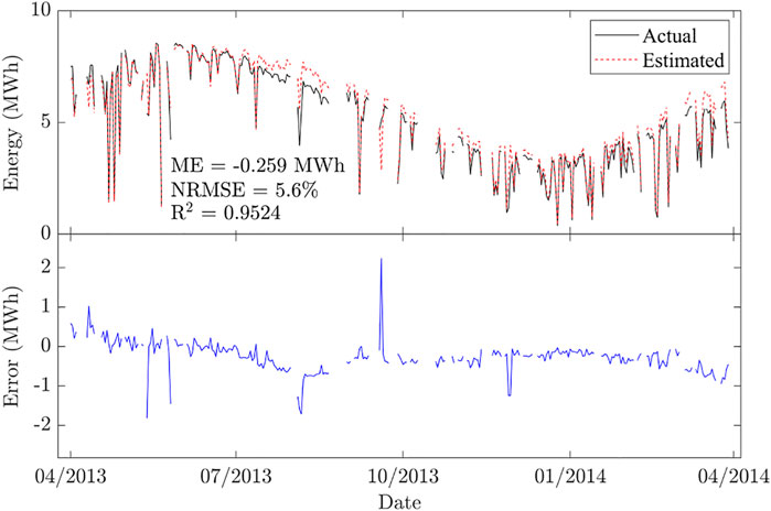
FIGURE 8. Validation for the parking’s PV field over the period of data.

FIGURE 9

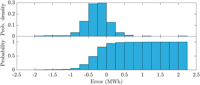
FIGURE 9. Ordinary and cumulative probability distribution histograms of the daily error for the parking’s PV field.

4 Discussion

PV (photovoltaic) production is useful to provide an example of how to deal with time-variant coefficients as posed in Section 2.2.2. Section 2.3.1 specifies how PV fields can be integrated within Ramos–Teodoro et al.’s (2018, 2020) modeling framework which was intended to be used in many applications where different energy carriers co-exist and need to be managed in an efficient way. Although Ramos–Teodoro et al. had already used the model presented here in previous studies (2018, 2020), it had not been formally described and validated until now. In such cases, both CIESOL and the parking’s facilities acted as producers in two different energy hubs with self-consumption where the decisions on the use of the electricity (consumption, storage, and trading with the public utility grid) need to be taken on an hourly basis.

Nevertheless, considering the results obtained earlier, the fact that the mean error is negative in both cases confronts with the fundamentals of the isotropic sky model, the conservative choice because the amount of radiation on sloped surfaces is underestimated. Unfortunately, the facilities are not prepared to measure such magnitude directly, which would open the door to calibrate the equations presented in Section 2.3.2 separately and then they could be used as “ground truth” to do the same with the subsequent equations (the model presented in Section 2.3.3 could be validated with the DC magnitudes as well measured by the inverters). This suggests possibilities for improving the model which is still enough accurate for control purposes, especially if compared with similar values of the coefficient of determination found in the literature just for the model of the modules (equivalent to the Section 2.3.3 of this article); Zhou et al. (2007) validated their model with values ranging from 0.96 to 0.98, using a single-diode model and data corresponding to four typical days of 2007, and Ma et al. (2014) reached values of up to 0.998, which the authors recognize to be “much higher than those seen in the literature,” by using a two-diode model and three example days of 2014. Analyzing more concrete electric parameters and over a longer period would help to enhance the accuracy of these models, which is a technical issue whose solution is underway for future publications.

Data Availability Statement

The raw data supporting the conclusion of this article will be made available by the authors, without undue reservation.

Author Contributions

All authors listed have made a substantial, direct, and intellectual contribution to the work and approved it for publication.

Funding

This work has been funded with the R&D Project the framework of the Feder-Andalucía 2014–2020 operational programme, UAL18-TEP-A055-B, of the Ministry of Economy, Knowledge, Business and University of the Andalusian Regional Government, the University of Almería, and ERDF funds.

Conflict of Interest

The authors declare that the research was conducted in the absence of any commercial or financial relationships that could be construed as a potential conflict of interest.

Publisher’s Note

All claims expressed in this article are solely those of the authors and do not necessarily represent those of their affiliated organizations, or those of the publisher, the editors, and the reviewers. Any product that may be evaluated in this article, or claim that may be made by its manufacturer, is not guaranteed or endorsed by the publisher.

Acknowledgments

The authors wish to thank the Elsamex S.A. and the CIESOL Research Center for providing real data of their facilities. They thank the reviewers as well for their valuable comments, which have helped to improve the quality of this study.

References

Castilla, M. d. M., Álvarez, J. D., Rodríguez, F., and Berenguel, M. (2014). “Comfort Control in Buildings,” in Advances in Industrial Control. London, United Kingdom: Springer-Verlag London. doi:10.1007/978-1-4471-6347-3

CrossRef Full Text | Google Scholar

Duffie, J. A., and Beckman, W. A. (2013). Solar Engineering of Thermal Processes. Hoboken, New Jersey, United States: John Wiley & Sons.

Google Scholar

Evins, R., Orehounig, K., Dorer, V., and Carmeliet, J. (2014). New Formulations of the 'energy Hub' Model to Address Operational Constraints. Energy 73, 387–398. doi:10.1016/j.energy.2014.06.029

CrossRef Full Text | Google Scholar

Evins, R. (2015). Multi-level Optimization of Building Design, Energy System Sizing and Operation. Energy 90, 1775–1789. doi:10.1016/j.energy.2015.07.007

CrossRef Full Text | Google Scholar

Geidl, M., and Andersson, G. (2007). Optimal Power Flow of Multiple Energy Carriers. IEEE Trans. Power Syst. 22, 145–155. doi:10.1109/tpwrs.2006.888988

CrossRef Full Text | Google Scholar

Gul, M., Kotak, Y., and Muneer, T. (2016). Review on Recent Trend of Solar Photovoltaic Technology. Energy Explor. Exploit. 34, 485–526. doi:10.1177/0144598716650552

CrossRef Full Text | Google Scholar

Kazem, H. A., and Yousif, J. H. (2017). Comparison of Prediction Methods of Photovoltaic Power System Production Using a Measured Dataset. Energ. Convers. Manage. 148, 1070–1081. doi:10.1016/j.enconman.2017.06.058

CrossRef Full Text | Google Scholar

Klein, S. A., Beckman, W. A., Mitchell, J. W., Duffie, J. A., Duffie, N. A., Freeman, T. L., et al. (2017). “TRNSYS 18: A Transient System Simulation Program. Technical Report,” in Solar Energy Laboratory (Madison, United States: University of Wisconsin).

Google Scholar

Ma, T., Yang, H., and Lu, L. (2014). Solar Photovoltaic System Modeling and Performance Prediction. Renew. Sustain. Energ. Rev. 36, 304–315. doi:10.1016/j.rser.2014.04.057

CrossRef Full Text | Google Scholar

Mohammadi, M., Noorollahi, Y., Mohammadi-Ivatloo, B., and Yousefi, H. (2017). Energy Hub: From a Model to a Concept - A Review. Renew. Sustain. Energ. Rev. 80, 1512–1527. doi:10.1016/j.rser.2017.07.030

CrossRef Full Text | Google Scholar

Ramos-Teodoro, J., Rodríguez, F., Berenguel, M., and Torres, J. L. (2018). Heterogeneous Resource Management in Energy Hubs with Self-Consumption: Contributions and Application Example. Appl. Energ. 229, 537–550. doi:10.1016/j.apenergy.2018.08.007

CrossRef Full Text | Google Scholar

Ramos-Teodoro, J., Giménez-Miralles, A., Rodríguez, F., and Berenguel, M. (2020). A Flexible Tool for Modeling and Optimal Dispatch of Resources in Agri-Energy Hubs. Sustainability 12, 8820. doi:10.3390/su12218820

CrossRef Full Text | Google Scholar

Ramos-Teodoro, J., Rodríguez, F., Pérez, M., and Berenguel, M. (2021). “A Comparative Study of Model Fitting for Estimating the Overall Efficiency of Grid-Connected Photovoltaic Inverters,” in Proceedings of the 19th International Conference on Renewable Energies and Power Quality, Almeria, Spain, 28–30 July, 2021. doi:10.24084/repqj19.292

CrossRef Full Text | Google Scholar

Zhou, W., Yang, H., and Fang, Z. (2007). A Novel Model for Photovoltaic Array Performance Prediction. Appl. Energ. 84, 1187–1198. doi:10.1016/j.apenergy.2007.04.006

CrossRef Full Text | Google Scholar