Signal-to-Noise Ratio Based Fault Detection and Identification

In this work, we introduce signal-to-noise ratio (SNR) based fault detection and identification mechanisms for a networked control system feedback loop, where the network component is represented by an additive white noise (AWN) channel. The SNR approach is known to be a steady-state analysis and design tool, thus we first introduce a finite time approximation for the estimated AWN channel SNR. We then consider the case of a general linear time-invariant plant model with one unstable pole. The potential faults that we discuss here cover simultaneously the plant model gain and/or the unstable pole. The fault detection is performed relative to the estimated AWN channel SNR. The fault identification is performed using recursive least squares ideas and then further validated with the observed SNR value, when a fault has been previously detected. We show that the proposed SNR-based fault mechanism (fault detection plus fault identification) is capable of processing the proposed faults. We conclude discussing future research based on the contributions exposed in the present work.

1 Introduction

Control theory, from the 20th century up to the 21st century, moved from what is known as classic control into new research areas such as networked control systems (NCSs). Theory and practice experts have been very busy (Chen et al., 2011), since results in NCSs are intrinsically multidisciplinary by definition, for example, by considering simultaneously established results in control and also information theory (Nair and Evans, 2004; Martins and Dahleh, 2008). Other examples joined linear optimal control results together with communication theory results (Elia, 2004; Braslavsky et al., 2007; Rojas, 2012) for additive white noise (AWN) channels. Similarly, an optimal approach for output tracking control over erasure channels has been proposed for stability and subject to model uncertainties in Jiang et al. (2021). In more recent years, we have also seen an increase in results that involve event-triggered NCS controllers (Heemels et al., 2012; da Silva et al., 2014; Campos-Delgado et al., 2015) which attempt to use limited available communication and energy resources with paucity, and nevertheless achieve a set of given goals, be those goals stability, performance, or robustness. These and other NCS results can constitute the foundation for a better control practice in the near future.

An NCS result, contributed early on in Braslavsky et al. (2007), imposes a channel input power constraint $\mathcal{P}$ for an AWN channel in a control feedback loop and then characterizes the infimal channel signal-to-noise ratio (SNR) in terms of the plant model features (unstable poles, non-minimum phase zeros, etc.). The resulting SNR expression can then be used to revisit the control feedback loop stability in terms of an SNR limitation, in particular when the controlled plant model is unstable. Specifically, the SNR fundamental limitation expressions contributed in Braslavsky et al. (2007) deal with unstable single-input single-output (SISO) linear time-invariant (LTI) plant models, both in continuous time and discrete time, characterizing the infimal channel input SNR bound required to achieve control feedback loop stability.

A large body of contributions also exist on the topic of fault detection and identification, with many books already written on these topics (Gertler, 1998; Chen and Patton, 1999; Blanke et al., 2003; Isermann, 2006; Saberi et al., 2007; Varga, 2017), together with informative review articles such as Ding et al. (2000) and Saberi et al. (2000). A fault is usually defined as an abnormal behavior occurring in a process, which in turn is of interest to first detect, identify, and then (ideally) properly recover from. There are different formulations for the problem of fault detection for LTI systems, which can be roughly categorized as approximate (such as the synthesis of fault detection filters subject to noise) and exact formulations (such as the nullspace method).

The variability inherent in NCSs might also be caused by anomalous variations in the plant model. An NCS example of the proposed setup is presented in Figure 1, where in this article we have considered a memoryless AWN communication channel in place of the communication network, specifically over the feedback path. These anomalous variations can be given the interpretation of faults, thus the need to develop a fault mechanism to detect and identify them (Figure 1) to later on inform a possible controller adaptation in order to achieve what is known as a fault-tolerant control feedback loop. Ding (2012) contributed a survey on NCS fault detection and fault-tolerant control. Another review on fault diagnosis for NCS can be found in Aubrun et al. (2008) with the objective of reducing performance degradation due to the different NCS communication features. A dynamic observer is designed for sensor fault detection under finite frequency disturbance and noise in a linear NCS (Dai et al., 2021). In Ren et al. (2018), an event-triggered H-infinity fault detection filter has been contributed in order to reduce unnecessary communication in the NCS dominated by time-varying latency and fading phenomena. A Bayesian approach, on the other hand, is the basis in Lami et al. (2020) for a fault detection proposal, in the context of an NCS irrigation canal application, while Li et al. (2009) use a Markov jumping linear system (MJLS) approach to define their residual generator. An NCS robust fault-tolerant control feedback loop is designed in Bahreini and Zarei (2019) with faults also modeled as MJLS, but with incomplete transition probabilities knowledge, for which Linear Matrix Inequalities based sufficient conditions are then presented as to ensure stochastic stability. In a multi-agent context, task allocation is proposed in Schenk and Lunze (2020) to achieve fault tolerance through the cooperation between a set of healthy and faulty agents, instead of focusing on recovering nominal performance; see also Wang et al. (2021). A nonlinear model predictive control, subject to random network latencies and random packet dropout phenomena, is used to design a fault-tolerant control feedback loop in Wang et al. (2016) based on a predictive observer with guaranteed input-to-state stability. On the other hand, a class of nonlinear NCSs, where the nonlinear terms is modeled using neural networks, has been studied by Ye et al. (2021), and LMIs are used to obtain the fault detection filter gains. Fault detection for nonlinear NCSs subject to random delays has also been considered when using the LMIs by Li et al. (2020), Huang and Pan (2020), and Gu and Yao (2021). Finally, a robust neural network-based controller was designed to detect and mitigate false data injection attacks (which can be interpreted as malicious faults) in Sargolzaei et al. (2020).

FIGURE 1

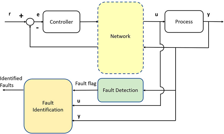
FIGURE 1. Networked control system (NCS) single-input single-output (SISO) feedback loop with fault detection and fault identification stages.

The current state of the art on fault mechanism designs for NCS still lacks the option of an SNR approach-based fault detection and identification mechanism. We also observe that most of the reported NCS contributions include a communication network simultaneously over the controller-to-plant (C2P) and the plant to controller (P2C) paths (Figure 1). However, when designing the NCS feedback loop, there is always the potential to collocate either the controller with the sensor devices, thus considering only the C2P path, or the controller with the plant model, and only then dealing with the P2C path for explicit AWN channel location. In this work, we focus on the P2C path, since for fault detection, the C2P path option, or the simultaneous presence of AWN communication channels in both locations, can be addressed in a similar manner.

Our first contribution in this article is to establish a fault detection algorithm to determine the occurrence of faults based on an finite time estimated AWN channel SNR. This for a SISO LTI plant model with one unstable pole. Our second contribution is to add to the previous detection algorithm, a fault identification stage using the recursive least square (RLS) algorithm which, upon a fault being flagged, can discriminate faults consistent with the estimated AWN channel SNR. We use examples, when appropriate, to further illustrate the proposed contributions.

This article is organized as follows: Section 2 presents the general assumptions, introducing the plant and AWN channel models. We also present here the AWN channel SNR deduction for a control feedback loop. Section 3 addresses the contributions of this work; that is, we define in full the proposed finite time AWN channel SNR estimation, the SNR-based fault detection stage and the fault identification stage for the proposed plant model. In Section 4, we discuss the possible avenues for generalization in future research of the presented results and summarize the present work.

2 Methods

In the following subsection, we proceed to list the assumptions for the present work.

2.1 Assumptions

–LTI plant model: The LTI plant model G(z) is assumed to be an LTI model given by

$G\left(z\right)=\frac{K}{z-\rho }\cdot G_s\left(z\right),(1)$

with $K\in {\mathbb{R}}^{+}$, |ρ| > 1 and G_s(z) is a known proper, stable rational transfer function.

–AWN channel model: The AWN channel model is characterized by its channel input power constraint $\mathcal{P}$ and channel additive noise n(k). The channel input power constraint is such that distortionless transmission is achieved both at nominal and faulty conditions.

–Channel additive noise process n(k): The channel additive noise process n(k) is assumed, to be in this work, as a zero mean, independent and identically distributed, white noise process. The noise variance σ² is assumed to be known.

– Reference signal: The reference signal is assumed to be constant and of value $r\in \mathbb{R}$.

The plant LTI model, AWN channel model, and channel additive noise process assumptions are in line with the SNR approach and can be traced to the seminal work of Braslavsky et al. (2007). The reference signal is adapted from the work of Rojas (2021).

2.2 Signal-to-Noise Ratio Constrained Control Approach

We now proceed to illustrate the SNR constrained control approach. For this, we take the case of r = 0.

From Figure 2, we have that the channel input power $\mathcal{P}$ is calculated as $\Vert y{\Vert }_{Pow}^2\triangleq {\lim }_{k\to \infty }\mathcal{E}\left\{y^2(k)\right\}$. The power at the plant output $\Vert y{\Vert }_{Pow}^2$, to guarantee a distortionless transmission, cannot exceed the channel input power constraint $\mathcal{P}>\Vert y{\Vert }_{Pow}^2$. Under stationary condition (see Åström, 1970, §4.2), the channel input power can also be stated as $\Vert y{\Vert }_{Pow}^2={‖T(z)‖}_2^2{\sigma }^2$, where

$T\left(z\right)=\frac{C\left(z\right)G\left(z\right)}{1+C\left(z\right)G\left(z\right)}.(2)$

FIGURE 2

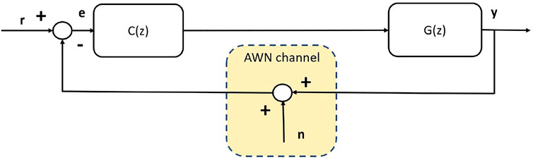
FIGURE 2. NCS SISO feedback loop with AWN channel over the P2C path.

Here T(z) is the complementary sensitivity function feedback loop transfer function with output y(k) and input r(k). We can then restate the channel input power inequality as an SNR inequality by means of the H₂ norm of T(z)

$\frac{\mathcal{P}}{{\sigma }^2}>\underset{C\in \mathcal{K}}{\min }{‖T‖}_2^2,(3)$

where $\mathcal{K}$ is the set of stabilizing controllers. From the previous equation, we have that the SNR inequality highlights a lower bound defined over the set of stabilizing controllers $\mathcal{K}$; for example, see Rojas (2012). When the plant model is unstable, this lower bound cannot be zero and thus will become a fundamental limitation for unstable plant models.

2.3 Finite Time Approximation

For designing a fault detection scheme, we cannot in practice guarantee k → ∞ to compute the channel input power definition from the available measurement of y(k). To achieve this, we introduce the following definition:

Definition 1. L is the sample length on which the stationarity assumption for the control feedback loop signals (in particular, the channel input signal) holds for a given tolerance value ϵ defined by the user.Based on Definition 1, we then propose an L sample length moving average of the channel input signal y(k) as its finite time approximation version

$y_L\left(k\right)=\frac{{\sum }_{i=k+1}^{k+L}y\left(i\right)}{L}.(4)$

We are then left with appropriately selecting the value of L. For this, we propose to use the averaged signal variance such that ${\sigma }_{y_L}^2\le ϵ$ for a given tolerance value ϵ defined by the user. To perform this selection of L, we then introduce Algorithm 1.

Algorithm 1. Estimation of L.Starting with the initialization stage, Algorithm 1 runs an outer for loop of a simulation based on Figure 2, evaluating the infimal SNR over an AWN channel over the P2C path (using, for example, MATLAB). Then, the inner for loop retrieves the simulated output vector y(k) data to repeat the y_L calculation a total of N times over a rolling time-window of selected length L, from Tss + k + 1 to Tss + k + L. T_ss is a time value set so as to avoid any initial conditions in transient. The selections for the inner for loop will test the candidate value of L through a specific channel noise realization, when the closed-loop dynamics have settled (by means of T_ss). The outer for loop completes the algorithm by averaging the selection of L through a number of noise realizations determined by the parameter iter and by testing the ϵ stopping condition with the sample variance of y_L(k) obtained from the inner loop. If the sample variance fails the test, then we add one to the working value of L and repeat each of the steps. If the sample variance satisfies the ϵ stopping condition, we then output the last working value L as the selected time window length in Eq. 4.

3 Results

By considering the value of L settled using Algorithm 1, we now move on into providing a lemma for SNR-based fault detection.

Lemma 1. SNR Fault Detection. The Fault Flag (FF) variable is raised to 1 when a fault is detected in an NCS feedback loop as shown in Figure 2; that is,

$FF\left(k\right)=\left\{\begin{array}{ccc}\hfill 0\hfill & \hfill if\hfill & \hfill SN{R}_L\left(k\right)\le {\mathrm{\Gamma }}_o\pm \mathcal{C}\hfill \\ \hfill 1\hfill & \hfill if\hfill & \hfill SN{R}_L\left(k\right)>{\mathrm{\Gamma }}_o\pm \mathcal{C}\hfill \end{array}\right.,(5)$

where SNR_L(k) is the finite time SNR approximation defined as

$\Vert y{\Vert }_{Pow}^2\approx SN{R}_L\left(k\right)\triangleq \frac{{\sum }_{j=k-L+1}^k{y}^2\left(j\right)}{L},(6)$

and Γ_o is the nominal theoretical SNR (with no faults), with L chosen using Algorithm 1. In turn, the confidence level $\mathcal{C}$ is selected as

$\mathcal{C}=\alpha \frac{{\sigma }_y}{\sigma },(7)$

equal to α times the ratio between σ_y, the theoretical stationary standard deviation of the channel input y(k), and σ, the channel noise n(k) standard deviation.The fault detection mechanism proposed in Lemma 1 constitutes the first contribution of the present work.

Remark 1. We observe that the proposed SNR fault detection mechanism is transparent to the simultaneous presence of the AWN channels over the C2P and P2C paths. The presence of both AWN channels will result in a different value of Γ_o, which is predicted to be (for example, see Rojas, 2013):

${\mathrm{\Gamma }}_o=T_o{\left(1\right)}^2\frac{r^2}{{\sigma }_{P2C}^2}+\Vert S_{o}G{\Vert }_2^2\frac{{\sigma }_{C2P}^2}{{\sigma }_{P2C}^2}+\Vert T_o{\Vert }_2^2,(8)$

where T_o(z) is the nominal complementary sensitivity (without faults), ${\sigma }_{C2P}^2$ is the C2P additive channel noise variance, and ${\sigma }_{P2C}^2$ is the P2C additive channel noise variance.

Remark 2. Since $\Vert y{\Vert }_{Pow}^2=\mathcal{E}\{y^2\}={\sigma }_y^2+{\mu }_y^2$ and ${\mu }_y^2=|T_o(1){|}_2^2{r}^2$, we have ${\sigma }_y^2=\Vert T_o{\Vert }_2^2{\sigma }^2$. Thus, the confidence level defined in Eq. 7 can be interpreted as the ratio between the feedback loop channel input power part due to the channel noise and the channel noise variance, which can then be rewritten as

$\mathcal{C}=\alpha \Vert T_o{\Vert }_2.(9)$

Remark 3. The value of α, on the other hand, is a design parameter for the fault detection mechanism, highlighting a trade-off between the rate of false positive fault detection (detecting a fault when there is none) and false negative detection (not detecting a fault when there is one). Therefore, the α parameter needs to be selected with care depending on the specific problem. If α is too small, then the noise level will trigger more false positive detections. This could still be traded-off against a larger value of L, but would imply an increased delay in detecting a fault when it occurs, due to the need of averaging a larger number of samples to obtain SNR_L. On the other hand, if the value of α is too large, there will be an opposite effect; that is, it would increase the occurrence of false negatives (the claim that there is no fault when there is really one). We would expect that if the expected fault SNR level is big with respect to the nominal SNR level Γ_o, then larger values of α could be used because there would be a less likelihood of false negatives. On the other hand, if there exists previous information of a smaller fault SNR level with respect to the nominal SNR level Γ_o, then a smaller α should be used, with a lower limit imposed by the presence of the channel noise.

Remark 4. We observe that the SNR approach behind Lemma 1 is a stationary approach. As a consequence, assuming stability of the control feedback loop, the same proposed detection mechanism could potentially be applied to nonlinear plant models, since it is well known that a nonlinear state trajectory can be approximated by a linear state trajectory in the vicinity of a stable equilibrium point.We now address, in the next lemma, our second contribution which consists of adding to the previous SNR-based detection algorithm a fault identification stage based on the process identification RLS algorithm.

Lemma 2. Fault Identification. Consider that a fault takes place in the plant model Eq. 1 due to a simultaneous change ΔK in the value of K and Δρ in the value of ρ when in feedback loop (Figure 2) with the controller defined as

$C\left(z\right)=\frac{\left({\rho }^2-1\right)}{\rho K}\cdot \left(1+\frac{K_{i}z}{z-1}\right)\cdot G_s^{-1}\left(z\right),(10)$

where K_i is known as the integral action gain. The above controller is assumed to stabilize the nominal feedback loop and the faulty feedback loop. The fault identification mechanism (Figure 1) has access to the values of u(k) and y(k) and can identify the fault values ΔK and Δρ, when the FF(k) in (Eq. 5) is 1, by means of a finite memory recursive least square (FM-RLS) algorithm as

$\begin{array}{l}\hfill \left[\begin{array}{c}\hfill \mathrm{\Delta }K\hfill \\ \hfill \mathrm{\Delta }\rho \hfill \end{array}\right]=\left[\begin{array}{c}\hfill K\hfill \\ \hfill \rho \hfill \end{array}\right]-{\left(\left[\begin{array}{ccc}\hfill u_s\left(k-L-1\right)\hfill & \hfill \dots \hfill & \hfill u_s\left(k-1\right)\hfill \\ \hfill y\left(k-L-1\right)\hfill & \hfill \dots \hfill & \hfill y\left(k-1\right)\hfill \end{array}\right]\cdot \left[\begin{array}{cc}\hfill u_s\left(k-L-1\right)\hfill & \hfill y\left(k-L-1\right)\hfill \\ \hfill ⋮\hfill & \hfill ⋮\hfill \\ \hfill u_s\left(k-1\right)\hfill & \hfill y\left(k-1\right)\hfill \end{array}\right]\right)}^{-1}\cdot \\ \hfill \cdot \left[\begin{array}{ccc}\hfill u_s\left(k-L-1\right)\hfill & \hfill \dots \hfill & \hfill u_s\left(k-1\right)\hfill \\ \hfill y\left(k-L-1\right)\hfill & \hfill \dots \hfill & \hfill y\left(k-1\right)\hfill \end{array}\right]\left[\begin{array}{c}\hfill y\left(k-L\right)\hfill \\ \hfill ⋮\hfill \\ \hfill y\left(k\right)\hfill \end{array}\right],\end{array}(11)$

where u_s(k) is the output of the stable part of the plant model, that is, u_s(k) = g_s(k) ∗ u(k), with $g_s(k)={\mathcal{Z}}^{-1}\{G_s(z)\}$.

Proof. When the AWN channel is over the P2C path, the complementary sensitivity function describes the feedback loop relationship between y(k) and n(k) (bar a negative sign), as well as the feedback loop relationship between y(k) and r(k). Given the proposed controller structure, the theoretical channel SNR will be defined as

${\mathrm{\Gamma }}_o=\frac{\Vert y{\Vert }_{Pow}^2}{{\sigma }^2}=\Vert T_o{\Vert }_2^2+\frac{r^2}{{\sigma }^2}.(12)$

Due to the channel noise being white, we satisfy the condition of persistent excitation for closed loop identification. In the presence of a fault due to a simultaneous change ΔK and Δρ, if signals y(k) and u(k) are available, then it is a matter of observing the correct regressor matrix to identify the changing values of the parameters K(k) and ρ(k) (time-varying values due to the faults) together with a FM-RLS. The use of process identification methods, such as RLS, for a correct fault identification is suggested, for example, in Isermann (2006, Ch. 9). Observing that G_s(z), the stable part of the plant model, is not subject to change, we can then filter u(k) and obtain u_s(k) = g_s(k) ∗ u(k). The resulting regressor matrix for a vector parameter $\theta ={\left[\begin{array}{cc}\hfill K(k)\hfill & \hfill \rho (k)\hfill \end{array}\right]}^T$, with memory length L, is then given by:

${\mathrm{\Phi }}_L=\left[\begin{array}{cc}\hfill u_s\left(k-L-1\right)\hfill & \hfill y\left(k-L-1\right)\hfill \\ \hfill ⋮\hfill & \hfill ⋮\hfill \\ \hfill u_s\left(k-1\right)\hfill & \hfill y\left(k-1\right)\hfill \end{array}\right].(13)$

The estimated parameters vector is then $\widehat{\theta }={\left({\mathrm{\Phi }}_L^T\cdot {\mathrm{\Phi }}_L\right)}^{-1}{\mathrm{\Phi }}_L^T\vec{y}$ as in Eq. 11, with $\vec{y}={\left[\begin{array}{ccc}\hfill y(k-L)\hfill & \hfill \dots \hfill & \hfill y(k)\hfill \end{array}\right]}^T$ which concludes the proof.The fault identification mechanism proposed in Lemma 2 constitutes the second contribution of the present work. We now illustrate these two mechanisms with an example.

Example 1. We proceed with the present example by stating the values for the proposed parameters of this example in Table 1.The parameters values in Table 1 are a representative selection. The greater the values of r, ρ, and K, the greater value of the nominal SNR Γ_o. The values of the parameters iter, Tsim, and ϵ related to Algorithm 1 are such that we achieve convergence of L to the value of 92. The plant model parameters G_s(z) and controller C(z) are such that we have control feedback loop stability at nominal and faulty conditions. The controller C(z) contains integral action to achieve reference signal tracking.In Figure 3, we have the numerical evaluation for the proposed plant model:

$G\left(z\right)=\frac{2\left(z-0.3\right)}{\left(z-3\right)\left(z-0.1\right)}(14)$

The plant model has one unstable pole as to have nominal SNR Γ_o greater than one (see Braslavsky et al., 2007 for more details). The other pole and transmission zero are stable.The plant model in Eq. 14 is then put in a feedback loop together with the proposed controller:

$C\left(z\right)=\frac{4}{3}\frac{\left(1.05z-1\right)\left(z-0.1\right)}{\left(z-1\right)\left(z-0.3\right)}.(15)$

The proposed controller above is such that it grants tracking of the proposed constant reference signal r = 1 due to the pole at z = 1, as well as invert cancel out the stable part G_s(z) of the plant model.As the iterations in Algorithm 1 increase (Figure 3), the L value for the finite time approximation is tested and, failing the comparison with the stop value of ϵ, is then increased to the final selected value of L = 92 after the set of 500 iterations. It is reasonable to assume convergence is achieved, since for the last 300 iterations, the value of L grew less than 10%. Notice from Figure 3 that the value of L is also effectively updated when the variance of y_L(k) exceeds the threshold limit defined by ϵ in Table 1(shown by the horizontal orange dashed line).We consider the effect of two faults for the proposed time model, described by the values in Table 2.Observe that the proposed faults focus on ΔK, which can be interpreted as an input fault, and on Δρ, which is a fault that more directly affects the SNR level under faulty conditions. We do not consider here, and leave as future research, the case of fault changes on the stable part G_s(z) of the plant model since this would affect the controller stable cancellation of it and might result in an unstable control feedback loop under faulty conditions.The feedback loop starts in the nominal condition until time sample k = 5,000 when the first fault, described by the pair (ΔK₁, Δρ₁), takes place. The first fault ends at time sample k = 10,000, recovering nominal conditions. At time sample k = 15,000, the second fault described by the pair (ΔK₂, Δρ₂) now takes place up to time sample k = 20,000. We then recover again nominal conditions up to time sample 25,000 when the simulation concludes. The theoretical SNR at nominal conditions is 9.9474, whereas the theoretical SNR under the first fault condition is 60.7302, while the theoretical SNR for the second fault is 60.9940.We now consider the application of Lemma 1 to detect the proposed faults. Notice that with G(z) in Eq. 14 and the controller C(z) in Eq. 15, the nominal feedback loop complementary sensitivity T_o will have an H₂ norm of 2.9912. Thus, the confidence level is obtained as $\mathcal{C}=5.9824$. In Figure 4A, we report the estimated finite time SNR_L, from an output signal y(k) realization, when the feedback loop is subjected to the two described faults, shown as a blue solid line. The use of Lemma 1 is reported by an orange solid line, and correctly reports the fault occurrences, with a few instances of false negative detections (not detecting a fault when a fault is present) and instances of false positive detections (detecting a fault when no fault is present) at the end of each fault period.To illustrate the trade-off behind the value of α selection, we test the confidence level for different values of α versus false positives and false negative probabilities in Figure 4B. We also report in Figure 4A two examples of how the confidence level affects the two occurrences of false negatives and false positives, for alternative values of α = 1, black solid line, and α = 4, green solid line. As α increases, and thus the confidence level $\mathcal{C}$ also increases, the fault positive probability (defined as the ratio between the number of fault positive samples and the number of samples under nominal conditions) decreases, blue solid line in Figure 4B. However, as α increases, and the confidence level $\mathcal{C}$ increases, we now have that the fault negative probability (defined as the ratio between the number of fault negative samples and the number of samples under faulty conditions) increases, red dashed line in Figure 4B. Clearly, the best value of α to set the confidence level $\mathcal{C}$ is one that trades off the improvement in false positive probability reduction versus false negative probability reduction, which corresponds to the α value when the two lines cross each other. For this example, this value is approximately 2.5. This confirms, a posteriori, that the working choice of α = 2, was reasonable.Once a fault has been detected, we now use Lemma 2 to identify the said faults. In Figure 5, we report the successful identification of both faults using the proposed FM-RLS approach. The result is quite good for both parameters, but it is not instantaneous as the zooming on the right panels in Figure 5 show. In this identification, there is another trade-off between the value of L, the quality of the identification, and the lag in correctly identifying the amount of the fault, ΔK and/or Δρ. The bigger the value of L, the better the quality, the longer the lag, and vice versa. Observe that, after the recursive estimates have settled, the identified fault parameters are the exact values reported in Table 2. Thus, if we were to check the expected SNR under these two identified faults, we would observe values that would be in agreement with the SNR_L previously observed in Figure 4A during faults.The successful use of Lemma 2 as reported in Figure 5 is tied to having access to signal u(k) at the process input (Figure 1). However, the presence of an AWN channel model over the P2C path, as in Figure 2, suggests that signal u(k) can only be available at the same location as signal y(k) (to then inject into the fault identification mechanism) if transmitted by an independent network. This is so because if u(k) was perfectly available at the process output, it would mean that the controller is also collocated with the plant output, and then there would be no real need for an AWN channel model over the feedback loop. We test this in Figure 6, by assuming that u(k) is transmitted through a secondary AWN channel model with independent noise channel with respect to the already stated AWN channel model over the P2C path. The channel noise variance of this secondary AWN channel is assumed to be 2% of σ², and even for this, the application of Lemma 2 considering this transmitted version of u(k) results in far more noisier and biased estimates of the two faults; see the left panels in Figure 6. The bias effect can be ameliorated somehow by evaluating it during the nominal operation (no faults) and then subtracting it from the obtained estimations when the faults are present; see the right panels in Figure 6. We can observe from the same figure for these two faults that ΔK is the fault component that is most affected by the noise presence in u(k). This suggests that to implement a fault identification mechanism based on Lemma 2, the transmission quality for the signal u(k) needs to be in the order of magnitudes better than the ones operating inside the feedback loop.

TABLE 1

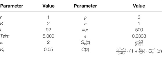
TABLE 1. Parameters values for Example 1.

FIGURE 3

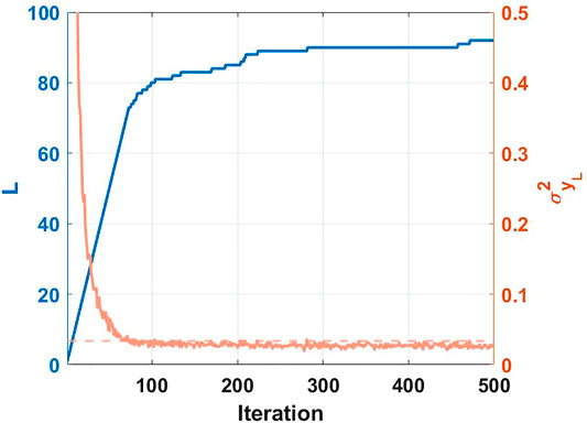
FIGURE 3. Evolution of the estimated value of L as per Algorithm 1.

TABLE 2

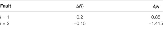
TABLE 2. Fault values for example 1.

FIGURE 4

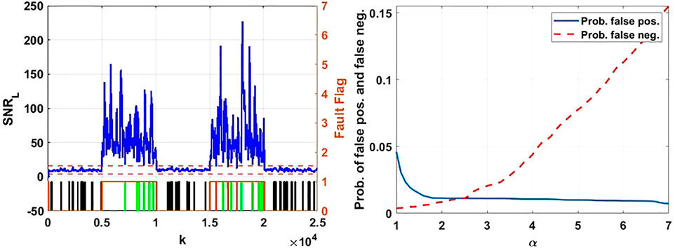
FIGURE 4. (A) Estimated finite time SNR_L, blue solid line. Fault flag variable FF for α = 1, solid black line; for α = 2, solid orange line; and for α = 4, solid green line. (B) Evaluation of false positive probability, blue solid line, and false negative probability, red dashed line, as functions of α.

FIGURE 5

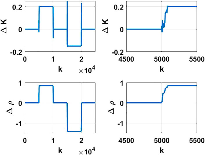
FIGURE 5. ΔK(k) and Δρ(k) estimates, left panels. Zoom on the estimates at the start of the first fault, right panels.

FIGURE 6

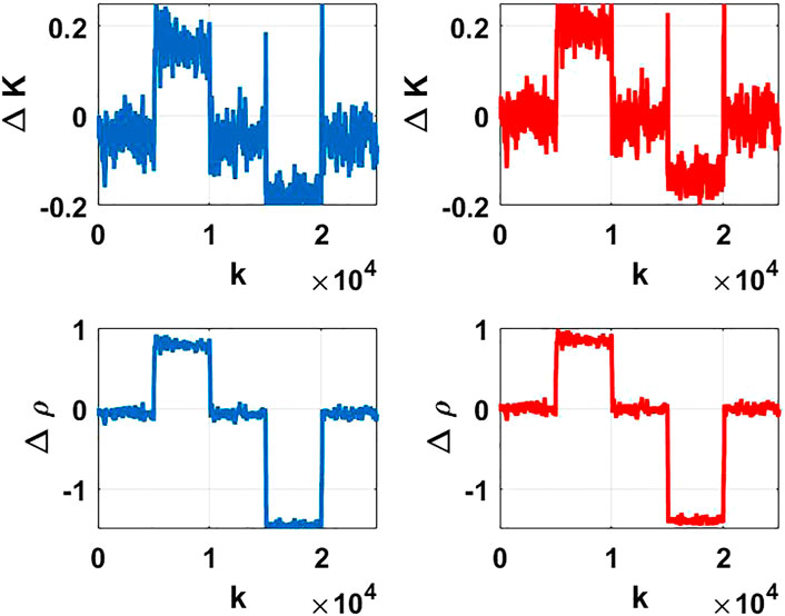
FIGURE 6. ΔK(k) and Δρ(k) estimates with noisy u(k), left panels in blue. Detrended ΔK(k) and Δρ(k) estimates with noisy u(k), left panels in red.

4 Discussion

In this work, we present an SNR-based fault detection and fault identification mechanisms for an NCS feedback loop, when the network is represented by an AWN channel over the P2C path. To the best of the authors' knowledge, the stated contribution is novel in as much that in the current state of the art no fault mechanism designs for NCS uses the SNR approach nor deals with the AWN channel model. The steady-state SNR approach required the introduction of a finite time approximation to estimate the relevant feedback loop signals, which we developed here. We also considered a fairly general LTI plant model containing one unstable pole. The faults that we studied were represented by sudden changes in both the plant model gain and/or the unstable pole values. The fault detection was achieved comparing with Γ_o, the AWN channel nominal SNR over the P2C path. The effect of the inclusion of an optimal tracking objective or the potential inclusion of simultaneous channels in the C2P and P2C paths can also readily be included in the proposed SNR of the AWN channel nominal SNR over the P2C value Γ_o.

On the other hand, the fault identification was performed here using an FM-RLS approach, when a fault has been previously detected. We showed with an example that the proposed SNR-based fault mechanism (fault detection plus fault identification) was capable of processing the proposed faults, with the caveat of almost perfect access to the signal u(k) at the process input. The SNR-based fault detection mechanism was not compared with other NCS-based fault mechanisms because, as far as the authors have surmised from the current state of the art, no other comparable results exist for AWN channel models subject to a power constraint (the core of the SNR approach). There are indeed other fault detection and identification solutions for NCS, as presented in the Introduction, but they focus on different communication features (channel latencies, erasure, fading, etc.). More so, even if a comparison with other NCS fault detection results was feasible, considering the result of Example 1, the fault detection response of our contribution successfully detects the proposed faults, and other methods could only perform equally as good. This is in the on-off nature of the fault detection question, either there is a fault or not, and at best, the answer from any other method would be the same. With respect to the SNR-based fault identification mechanism, the comparison with other methods could indeed be more nuanced, but again considering the results in Figure 6, we obtained an excellent fault identification result when using the FM-RLS approach here, a performance which could only be tied at best by other current NCS fault identification methods if they were actually comparable (which they are not, because they consider different communication network features, than additive channel noise and channel input power constraint).

Future research should consider relaxing the requirement on u(k) for fault identification, propose a different fault identification mechanism using perhaps a priori knowledge on the types of faults to be expected, the case of fault changes on the stable part G_s(z) of the plant model, and consider the case of other types of communication channel models. For example, if we want to consider optimal output tracking over erasure channels, we can adapt the results in Jiang et al. (2021) to obtain a new analytical expression for a power constraint expression akin to Γ_o.

Data Availability Statement

The raw data supporting the conclusion of this article will be made available by the authors, without undue reservation.

Author Contributions

All authors listed have made a substantial, direct, and intellectual contribution to the work and approved it for publication.

Funding

The authors are thankful to the Chilean Research Agency ANID for its support through Project Grant FONDECYT Regular No. 1190196 and Basal Project FB0008.

Conflict of Interest

The authors declare that the research was conducted in the absence of any commercial or financial relationships that could be construed as a potential conflict of interest.

Publisher’s Note

All claims expressed in this article are solely those of the authors and do not necessarily represent those of their affiliated organizations, or those of the publisher, the editors, and the reviewers. Any product that may be evaluated in this article, or claim that may be made by its manufacturer, is not guaranteed or endorsed by the publisher.

References

Åström, K. (1970). Introduction to Stochastic Control Theory. Cambridge, MA, USA: Academic Press.

Google Scholar

Aubrun, C., Sauter, D., and Yamé, J. (2008). Fault Diagnosis of Networked Control Systems. Int. J. Appl. Maths. Comput. Sci. 18, 525–538. doi:10.2478/v10006-008-0046-3

CrossRef Full Text | Google Scholar

Bahreini, M., and Zarei, J. (2019). Robust Fault-Tolerant Control for Networked Control Systems Subject to Random Delays via Static-Output Feedback. ISA Trans. 86, 153–162. doi:10.1016/j.isatra.2018.10.034

PubMed Abstract | CrossRef Full Text | Google Scholar

Blanke, M., Kinnaert, M., Lunze, J., and Staroswiecki, M. (2003). Diagnosis and Fault-Tolerant Control. Berlin: Springer-Verlag.

Google Scholar

Braslavsky, J. H., Middleton, R. H., and Freudenberg, J. S. (2007). Feedback Stabilization over Signal-To-Noise Ratio Constrained Channels. IEEE Trans. Automat. Contr. 52, 1391–1403. doi:10.1109/tac.2007.902739

CrossRef Full Text | Google Scholar

Campos-Delgado, D. U., Rojas, A. J., Luna-Rivera, J. M., and Gutiérrez, C. A. (2015). Event-triggered Feedback for Power Allocation in Wireless Networks. IET Control. Theor. Appl. 9, 2066–2074.

Google Scholar

Chen, J., de Silva, C., Olariu, S., Paschalidis, I. C., and Stojmenovic, I. (2011). “IEEE Transactions on Automatic Control,” in Special Issue on Wireless Sensor and Actuator Networks, Vol. 56.

Google Scholar

Chen, J., and Patton, R. J. (1999). Robust Model-Based Fault Diagnosis for Dynamic Systems. London: Kluwer Academic Publishers.

Google Scholar

da Silva, J. M. G., Lages, W. F., and Sbarbaro, D. (2014). “Event-triggered PI Control Design,” in Proceedings of the 19th IFAC World Congress, Cape Town, South Africa, 6947–6952. doi:10.3182/20140824-6-za-1003.01824IFAC Proc. Volumes47

CrossRef Full Text | Google Scholar

Dai, X.-W., Zheng, Z.-D., Gao, Y., Cui, D.-L., and Zhao, H.-T. (2021). Pole-zero Optimization Design of Dynamic Observer for Fault Detection of Networked Control Systems. Kongzhi Yu Juece/Control Decis. 36, 1351–1360.

Google Scholar

Ding, S. X. (2012). A Survey of Fault-Tolerant Networked Control System Design. IFAC Proc. Volumes 45, 874–885. doi:10.3182/20120829-3-mx-2028.00259

CrossRef Full Text | Google Scholar

Ding, S. X., Jeinsch, T., Frank, P. M., and Ding, E. L. (2000). A Unified Approach to the Optimization of Fault Detection Systems. Int. J. Adapt. Control. Signal. Process. 14, 725–745. doi:10.1002/1099-1115(200011)14:7<725::aid-acs618>3.0.co;2-q

CrossRef Full Text | Google Scholar

Elia, N. (2004). When Bode Meets Shannon: Control-Oriented Feedback Communication Schemes. IEEE Trans. Automat. Contr. 49, 1477–1488. doi:10.1109/tac.2004.834119

CrossRef Full Text | Google Scholar

Gertler, J. (1998). Fault Detection and Diagnosis in Engineering Systems. New York: Marcel Dekker.

Google Scholar

Gu, Z., and Yao, L. (2021). Fault Diagnosis and Fault‐tolerant Control of Uncertain Network Control Systems. Int. J. Adapt Control. Signal. Process. 35, 1941–1956. doi:10.1002/acs.3300

CrossRef Full Text | Google Scholar

Heemels, W., Johansson, K., and Tabuada, P. (2012). “An Introduction to Event-Triggered and Self-Triggered Control,” in Proceedings of the 51th Conference on Decision and Control, 3270–3285. doi:10.1109/cdc.2012.6425820

CrossRef Full Text | Google Scholar

Huang, K., and Pan, F. (2020). Fault Detection for Nonlinear Networked Control Systems with Sensor Saturation and Random Faults. IEEE Access 8, 92541–92551. doi:10.1109/access.2020.2992540

CrossRef Full Text | Google Scholar

Isermann, R. (2006). Fault-Diagnosis Systems. Berlin, Germany: Springer.

Google Scholar

Jiang, X., Chi, M., Chen, X., Yan, H., and Huang, T. (2021). Output Tracking Control Performance of Discrete Networked Systems over Erasure Channel with Model Uncertainty. IEEE Trans. Cybern., 1–9. In Press. doi:10.1109/tcyb.2021.3053010

CrossRef Full Text | Google Scholar

Lami, Y., Lefevre, L., Lagreze, A., and Genon-Catalot, D. (2020). “A Bayesian Approach for Fault Diagnosis in an Irrigation Canal,” in 24th International Conference on System Theory, Control and Computing, Sinaia, Romania, 328–335. doi:10.1109/icstcc50638.2020.9259694

CrossRef Full Text | Google Scholar

Li, L., Yao, L., Jin, H., and Zhou, J. (2020). Fault Diagnosis and Fault‐tolerant Control Based on Laplace Transform for Nonlinear Networked Control Systems with Random Delay. Int. J. Robust Nonlinear Control. 30, 1223–1239. doi:10.1002/rnc.4823

CrossRef Full Text | Google Scholar

Li, W., Ding, S. X., and Ding, X. (2009). On Fault Detection Design for Networked Control Systems. IFAC Proc. Volumes 42, 792–797. doi:10.3182/20090630-4-es-2003.00130

CrossRef Full Text | Google Scholar

Martins, N. C., and Dahleh, M. A. (2008). Feedback Control in the Presence of Noisy Channels: "Bode-Like" Fundamental Limitations of Performance. IEEE Trans. Automat. Contr. 53, 1604–1615. doi:10.1109/tac.2008.929361

CrossRef Full Text | Google Scholar

Nair, G. N., and Evans, R. J. (2004). Stabilizability of Stochastic Linear Systems with Finite Feedback Data Rates. SIAM J. Control. Optim. 43, 413–436. doi:10.1137/s0363012902402116

CrossRef Full Text | Google Scholar

Ren, W., Sun, S., Hou, N., and Kang, C. (2018). Event-triggered Non-fragile H∞ Fault Detection for Discrete Time-Delayed Nonlinear Systems with Channel Fadings. J. Franklin Inst. 355, 436–457. doi:10.1016/j.jfranklin.2017.11.015

CrossRef Full Text | Google Scholar

Rojas, A. J. (2013). “Control over Direct and Feedback Path Signal-To-Noise Ratio Constrained Channels,” in 2013 American Control Conference, Washington, DC, USA, 3183–3188. doi:10.1109/acc.2013.6580320

CrossRef Full Text | Google Scholar

Rojas, A. J. (2021). “Signal-to-Noise Ratio Feedback Constraint for Non-zero Mean Noise Processes,” in IEEE ICA/ACCA 2021, Santiago, Chile, 1–6. doi:10.1109/icaacca51523.2021.9465244

CrossRef Full Text | Google Scholar

Rojas, A. J. (2012). Signal-to-noise Ratio Fundamental Limitations in the Discrete-Time Domain. Syst. Control. Lett. 61, 55–61. doi:10.1016/j.sysconle.2011.09.010

CrossRef Full Text | Google Scholar

Saberi, A., Stoorvogel, A. A., and Sannuti, P. (2007). Filtering Theory: With Applications to Fault Detection, Isolation, and Estimation. Basel: Birkhauser.

Google Scholar

Saberi, A., Stoorvogel, A. A., Sannuti, P., and Niemann, H. (2000). Fundamental Problems in Fault Detection and Identification. Int. J. Robust Nonlinear Control. 10, 1209–1236. doi:10.1002/1099-1239(20001215)10:14<1209::aid-rnc524>3.0.co;2-c

CrossRef Full Text | Google Scholar

Sargolzaei, A., Yazdani, K., Abbaspour, A., Crane, C. D., and Dixon, W. E. (2020). Detection and Mitigation of False Data Injection Attacks in Networked Control Systems. IEEE Trans. Ind. Inf. 16, 4281–4292. doi:10.1109/tii.2019.2952067

CrossRef Full Text | Google Scholar

Schenk, K., and Lunze, J. (2020). “Fault-Tolerant Task Allocation in Networked Control Systems,” in 28th Mediterranean Conference on Control and Automation, Saint-Raphael, France, 313–318. doi:10.1109/med48518.2020.9182977

CrossRef Full Text | Google Scholar

Varga, A. (2017). Solving Fault Diagnosis Problems: Linear Synthesis Techniques. Studies in Systems, Decision and Control. Berlin, Germany: Springer.

Google Scholar

Wang, B., Zhang, B., and Su, R. (2021). Optimal Tracking Cooperative Control for Cyber-Physical Systems: Dynamic Fault-Tolerant Control and Resilient Management. IEEE Trans. Ind. Inf. 17, 158–167. doi:10.1109/tii.2020.2965538

CrossRef Full Text | Google Scholar

Wang, T., Gao, H., and Qiu, J. (2016). A Combined Fault-Tolerant and Predictive Control for Network-Based Industrial Processes. IEEE Trans. Ind. Electron. 63, 2529–2536. doi:10.1109/tie.2016.2515073

CrossRef Full Text | Google Scholar

Ye, Z.-H., Ni, H.-J., Zhang, D., and Xue, H.-x. (2021). Neural Network-Based Fault Detection for Nonlinear Networked Systems with Uncertain Medium Access Constraint: Application to Motor Systems. ISA Trans. 111, 211–222. doi:10.1016/j.isatra.2020.11.003

PubMed Abstract | CrossRef Full Text | Google Scholar