Tuning of PIDD2 controllers for oscillatory systems with time delays

Proportional–integral–derivative (PID) control is a durable control technology that has been widely applied in the process control industry. However, PID controllers cannot achieve satisfactory performance for oscillatory systems with long time delays; thus, high-order controllers like the proportional–integral–double derivative (${PIDD}^2$) can be adopted to enhance the control performance. In this paper, we propose a tuning formula for the ${PIDD}^2$ controller for oscillatory systems with time delays and its practical implementation via an observer bandwidth-based state-space ${PIDD}^2$. Simulation results show that the state-space ${PIDD}^2$ controller tuned from the proposed formula trades-off among robustness, time domain performance, and measurement noise attenuation and can arrive at a better control effect than PID for oscillatory systems.

1 Introduction

Proportional–integral–derivative (PID) control is a durable control technology that has been widely applied in the process control industry (Kim and Lee, 2021). The principal reason is its relatively simple structure, which can be easily implemented, understood, and maintained in practical industry production processes. PID is so wildly used in process control system applications, and it is one of the important factors in the development of the industry (Borase et al., 2021). Hence, most studies in the field of process control have only focused on PID control, which includes intelligent PID (Chan et al., 2007; Gundes and Ozguler, 2007), fuzzy PID (Tzafestas and Papanikolopoulos, 1990; Jin et al., 2017), optimal PID (Halikias and Zolotas, 1999; Chao et al., 2019; Memon and Shao, 2020; Memon and Shao, 2021), adaptive PID control (Radke and Isermannt, 1987; Pan et al., 2007), and fractional-order PID (Zhao et al., 2005; Chevalier et al., 2019).

It is well-known that the oscillatory dynamics of the process have various features, and parameter tuning is complicated and difficult. To facilitate research, the oscillatory dynamics of the process can be modeled as the standard second-order process with a dead-time (SOPDT) model. Up to now, research on the tuning of the SOPDT system has been mostly restricted to PID. Weng et al. (1997) derived the tuning formula of the PID controller based on the gain and phase margin for the underdamped oscillatory system. The user-specified gain and phase margins can be adaptively achieved, but the trade-off optimization between stability and tracking performance is not designed. Wang et al. (1999) proposed a PID controller parameter tuning method based on the closed-loop pole assignment strategy of the root locus for the oscillatory system; the parameter design process is more complicated. Huang et al. (2000) proposed an inverse-based synthesis PID controller for the oscillatory system and analyzed its robustness by the gain and phase margins. However, the effect of noise was not considered. Basilio and Matos (2002) designed the PID controller for the underdamping system, but the controlled plant did not account for dead time. Oliveira and Vrančić (2012) addressed the problem of decreasing the overshoot by switching controllers for underdamped second-order systems, which is not convenient for practical engineering applications. Kurokawa et al. (2020) proposed an optimal trade-off PID control system for a SOPDT system, which does not consider the impact of measurement noise. The aforementioned literature reports are devoted to the study of the controller from the perspective of the frequency domain. Although some research has been carried out on PID controllers, it is still unclear whether or not PID can effectively handle oscillatory process uncertainties like disturbance and measurement noise. Furthermore, it may be necessary to manually adjust the PID controller for the step response of the oscillatory process through trial and error, which may inevitably result in inaccuracies. More importantly, it is difficult for the conventional PID controller to guarantee the stability of the oscillatory process with a time delay. The scenario is quite different from the step response of the non-oscillatory plant, where numerous well-known formulas exist (Lee et al., 1998; Skogestad and Grimholt, 2012; Garpinger et al., 2014). Therefore, it would be desirable if there are tuning criteria for the oscillatory plant with time delays to improve the performance of systems.

As an example, consider the following oscillatory system with a time delay ($G\left(s\right)$):

$\begin{array}{c}G\left(s\right)=\frac{1}{s^2+0.2s+1}{e}^{-s}\end{array}.(1)$

The dynamic response of SOPDT under the conventional PID (Huang et al., 2000) is shown in Figure 1 when a unit step reference signal (the amplitude is 1) is inserted at $t=0s$ and an input disturbance signal (the amplitude is 5) is inserted at $t=50s$. Controller parameters are $K_p=0.1;K_i=0.5;K_d=0.5;$ from Figure 1, we can see that although the tracking response of PID is acceptable, the rejection–disturbance response is still oscillatory, which is undesired.

FIGURE 1

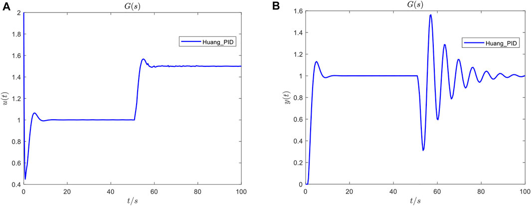
FIGURE 1. Dynamic response of the SOPDT model under PID: (A) controller output responses and (B) system output responses.

To improve the performance of conventional PID, a new conventional controller named the proportional−integral−double derivative (${PIDD}^2$) is widely used (kalyan and Suresh, 2021; Koley et al., 2020; Mokeddem and Mirjalili, 2020; Simanenkov et al., 2017; Sonkar and Rahi, 2016). The ${PIDD}^2$ controller is robust and capable of controlling the automatic voltage regulator under load frequency control system uncertainties (Mohanty, 2018; Chatterjee et al., 2019). So far, there are only some literature studies about parameter tuning for ${PIDD}^2$, e.g., CSA−${PIDD}^2$ (Koley et al., 2020), hFPA-PS−${PIDD}^2$ (Mohanty, 2020), GWO−${PIDD}^2$ (Kalyan, 2021), and Fuzzy−${PIDD}^2$ (Farooq et al., 2021). However, the ${PIDD}^2$ controller is not discussed for oscillatory systems. In reality, oscillatory systems are not subject to any special ${PIDD}^2$ tuning rules. To tune oscillatory SOPDT systems, this paper proposes the tuning formula of ${PIDD}^2$.

For practical implementation issues, we will investigate a state-space ${PIDD}^2$ control structure. The state-space ${PIDD}^2$ controller estimates the derivative of the controlled plant output via an observer. The second-order differentiation is utilized to reduce impacts of fluctuation of the disturbance. The state-space ${PIDD}^2$ controller retains the plant-independent property of the traditional PID and overcomes some of its disadvantages. For oscillatory systems with time delays, a tuning formula based on the state-space PIDD² controller is proposed first, and then, the parameters of ${PIDD}^2$ are obtained via the well-known internal model control (IMC) framework for oscillatory systems. The proposed tuning formula is tested for a wide variety of simulation examples and the load frequency control system. It is shown that the state-space ${PIDD}^2$ controller outperforms the traditional PID in oscillatory systems. The state-space ${PIDD}^2$ controller trades-off among disturbance rejection performance, robustness, and attenuation of the measurement noise.

The rest of the paper consists of four parts. In Section 2, ${PIDD}^2$ and its state-space implementation is introduced; tuning of the state-space ${PIDD}^2$ controller based on IMC for the SOPDT system is introduced in Section 3; Section 4 presents simulation and analysis results. Finally, conclusions are given in Section 5.

2 ${\mathit{P}\mathit{I}\mathit{D}\mathit{D}}^{\mathbf{2}}$ and its state-space implementation

A PID controller has been frequently utilized in the industry due to its simplicity and efficiency. The ${PIDD}^2$ controller has been used to enhance the performance of the conventional PID controller. The structure of ${PIDD}^2$ is similar to the conventional PID, in addition to the extra second-order derivative gain. An ideal ${PIDD}^2$ controller has the following transfer function form:

$\begin{array}{c}{C}_{PIDD}\left(s\right)=K_p+\frac{K_i}{s}+K_{d}s+K_{dd}{s}^2\end{array},(2)$

where $K_p$, $K_i$, $K_d,$ and $K_{dd}$ are the proportional variable, integral variable, derivative gain, and double derivative gain, respectively. ${PIDD}^2$ control can be written as a state-feedback control law, given as follows:

$\begin{array}{c}\begin{array}{l}u\left(t\right)=K_{dd}\left(\ddot{r}\left(t\right)-\ddot{y}\left(t\right)\right)+K_d\left(\dot{r}\left(t\right)-\dot{y}\left(t\right)\right)\\ +K_p\left(r\left(t\right)-y\left(t\right)\right)+K_i{\int }_0^t\left(r\left(\tau \right)-y\left(\tau \right)\right)d\tau \\ =:{\overline{K}}_o\left(\overline{r}\left(t\right)-x\left(t\right)\right).\end{array}\end{array}(3)$

Here, $y\left(t\right)$ is the controlled variable, $u\left(t\right)$ is the manipulated variable, and $r\left(t\right)$ is the reference signal.

$\begin{array}{c}\overline{r}\left(t\right)={\left[\begin{array}{c}\ddot{r}\left(t\right)\dot{r}\left(t\right)r\left(t\right){\int }_0^{t}r\left(\tau \right)d\end{array}\tau \right]}^T.\end{array}(4)$

The state vector is as follows:

$\begin{array}{c}x\left(t\right)={\left[\begin{array}{cc}\ddot{y}\left(t\right)\dot{y}\left(t\right)y\left(t\right)& {\int }_0^{t}y\left(\tau \right)d\tau \end{array}\right]}^T.\end{array}(5)$

The state-feedback gain is as follows:

$\begin{array}{c}{\overline{K}}_o=\left[\begin{array}{cccc}{K}_{dd}& K_d& K_p& K_i\end{array}\right].\end{array}(6)$

The state vector $x\left(t\right)$ (5) contains the derivative of $y\left(t\right)$, so it cannot be measured directly. An observer can be adopted to estimate it. Consider the following triple integral model:

$\begin{array}{c}\stackrel{\dots }{y}\left(t\right)=u\left(t\right).\end{array}(7)$

Let

$\begin{array}{c}{x}_1=\ddot{y},x_2=\dot{y,}{x}_3=y\end{array}.(8)$

Then, Eq. 7 can be written in the following state-space form:

$\begin{array}{c}\left\{\begin{array}{c}\left[\begin{array}{c}{\dot{x}}_1\\ {\dot{x}}_2\\ {\dot{x}}_3\end{array}\right]={\overline{A}}_o\left[\begin{array}{c}{x}_1\\ x_2\\ x_3\end{array}\right]+{\overline{B}}_{o}u,\\ y={\overline{C}}_o\left[\begin{array}{c}{x}_1\\ x_2\\ x_3\end{array}\right],\end{array}\right.\end{array}(9)$

where

$\begin{array}{c}{\overline{A}}_o=\left[\begin{array}{ccc}0& 0& 0\\ 1& 0& 0\\ 0& 1& 0\end{array}\right],{\overline{B}}_o=\left[\begin{array}{c}1\\ 0\\ 0\end{array}\right],{\overline{C}}_o=\left[\begin{array}{ccc}0& 0& 1\end{array}\right].\end{array}(10)$

Thus, the following Luenberger observer can be used to estimate ${\left[\begin{array}{ccc}\ddot{y}& \dot{y}& y\end{array}\right]}^T$.

$\left[\begin{array}{c}{\dot{\overline{x}}}_1\\ {\dot{\overline{x}}}_2\\ {\dot{\overline{x}}}_3\end{array}\right]=\left({\overline{A}}_o-\overline{L}{\overline{C}}_o\right)\left[\begin{array}{c}{\overline{x}}_1\\ {\overline{x}}_2\\ {\overline{x}}_3\end{array}\right]+{\overline{B}}_{o}u+\overline{L}y,(11)$

where $\overline{L}$ is the observer gain, which is given as follows:

$\begin{array}{c}\overline{L}={\left[\begin{array}{ccc}{\overline{\beta }}_1& {\overline{\beta }}_2& {\overline{\beta }}_3\end{array}\right]}^T.\end{array}(12)$

If $\overline{L}$ is chosen such that ${\overline{A}}_o-\overline{L}{\overline{C}}_o$ is asymptotically stable, then ${\widehat{\overline{x}}}_1\to \ddot{y}$, ${\widehat{\overline{x}}}_2\to \dot{y,}$ and ${\widehat{\overline{x}}}_3\to y$. Furthermore, ${\int }_0^{t}y\left(\tau \right)d\tau$ can be computed using another state ${\widehat{\overline{x}}}_4$, where

$\begin{array}{c}{\dot{\overline{x}}}_4={\overline{x}}_3=y\end{array}.(13)$

By combining Eq. 11 and Eq. 13, we have an estimation of the state vector of Eq. 5 with the following observer:

$\begin{array}{c}\dot{\overline{x}}=\left({\overline{A}}_e-{\overline{L}}_o{\overline{C}}_e\right)\overline{x}+{\overline{B}}_{e}u+{\overline{L}}_{o}y,\end{array}(14)$

where $\overline{x}={\left[\begin{array}{cccc}{\overline{x}}_1& {\overline{x}}_2& {\overline{x}}_3& {\overline{x}}_4\end{array}\right]}^T$ and

$\begin{array}{c}{\overline{A}}_e=\left[\begin{array}{cccc}0& 0& 0& 0\\ 1& 0& 0& 0\\ 0& 1& 0& 0\\ 0& 0& 1& 0\end{array}\right],{\overline{B}}_e=\left[\begin{array}{c}1\\ 0\\ 0\\ 0\end{array}\right],{\overline{C}}_e=\left[\begin{array}{cccc}0& 0& 1& 0\end{array}\right].\end{array}(15)$

${\overline{L}}_o$ is the observer gain vector shown as follows:

$\begin{array}{c}{\overline{L}}_o={\left[\begin{array}{cccc}{\overline{\beta }}_1& {\overline{\beta }}_2& {\overline{\beta }}_3& 1\end{array}\right]}^T\end{array}.(16)$

When ${\overline{L}}_o$ is chosen properly, ${\overline{A}}_e-{\overline{L}}_o{\overline{C}}_e$ is asymptotically stable, and

$\begin{array}{c}{\overline{x}}_1\left(t\right)\to \ddot{y}\left(t\right),{\overline{x}}_2\left(t\right)\to \dot{y}\left(t\right),{\overline{x}}_3\left(t\right)\to y\left(t\right),{\overline{x}}_4\left(t\right)\to {\int }_0^{t}y\left(\tau \right)d\tau .\end{array}(17)$

Hence, the third-order state-space PID is the implementation of ${PIDD}^2$, and an ideal ${PIDD}^2$ controller can be approximated with the following third-order state-space PID (SS-${PIDD}^2$) controller:

$\begin{array}{c}\{\begin{array}{c}\dot{\overline{x}}=\left({\overline{A}}_e-{\overline{L}}_o{\overline{C}}_e\right)\overline{x}+{\overline{B}}_{e}u+{\overline{L}}_{o}y,\\ u={\overline{K}}_o\left(\overline{r}-\overline{x}\right).\end{array}\end{array}(18)$

So the feedback controller from $y$ to $u$ is as follows:

$\begin{array}{c}\begin{array}{c}{K}_c\left(s\right)={\overline{K}}_o{\left(sI-{\overline{A}}_e+{\overline{B}}_e{\overline{K}}_o+{\overline{L}}_o{\overline{C}}_e\right)}^{-1}{\overline{L}}_o\\ =\frac{\left(K_{dd}{\overline{\beta }}_1+K_d{\overline{\beta }}_2+K_p{\overline{\beta }}_3+K_i\right)s^3+\left(K_d{\overline{\beta }}_1+K_p{\overline{\beta }}_2+K_i{\overline{\beta }}_3\right)s^2+\left(K_p{\overline{\beta }}_1+K_i{\overline{\beta }}_2\right)s+K_i{\overline{\beta }}_1}{s\left[s^3+\left(K_{dd}+{\overline{\beta }}_3\right)s^2+\left(K_{dd}{\overline{\beta }}_3+K_d+{\overline{\beta }}_2\right)s+{\overline{\beta }}_1+K_{dd}{\overline{\beta }}_2+K_d{\overline{\beta }}_3+K_p\right]}\end{array}\end{array}.(19)$

${\overline{K}}_o$ is the controller gain vector, as shown in Eq. 6.

Figure 2 shows the structural block diagram of the third-order state-space PID (SS-${PIDD}^2$). $\alpha$ is the set-point weight, which is used to reduce the overshoot. By default, $\alpha =1$.

FIGURE 2

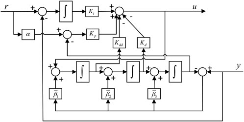
FIGURE 2. Block diagram of the state-space ${\mathit{P}\mathit{I}\mathit{D}\mathit{D}}^{\mathbf{2}}$ controller.

3 Tuning of the state-space ${\mathit{P}\mathit{I}\mathit{D}\mathit{D}}^{\mathbf{2}}$ controller based on IMC for the SOPDT system

The dynamics of the oscillatory SOPDT system is relatively complicated, and the controller parameter design process faces severe challenges. In general, the low-order controller often neglects the higher-order dynamics of oscillatory systems. Thus, the result of the control effect is not accurate (Wang et al., 2021). The well-known internal model control has the advantage of using one or two tuning parameters to achieve good control performance to model inaccuracies (Shamsuzzoha and Lee, 2007, p.). Therefore, in this section, we will discuss in detail how the parameters of the SS-${PIDD}^2$ controller are obtained using IMC.

3.1 Description of the internal model control (IMC)

Figure 3 shows the structural block diagram of the two-degree-of-freedom IMC (TDF-IMC) controller. $P\left(s\right)$ is the plant to be controlled, and $P_M\left(s\right)$ is the plant model; $Q\left(s\right)$ is the set-point tracking controller, and $Q_d\left(s\right)$ is the disturbance rejection controller.

FIGURE 3

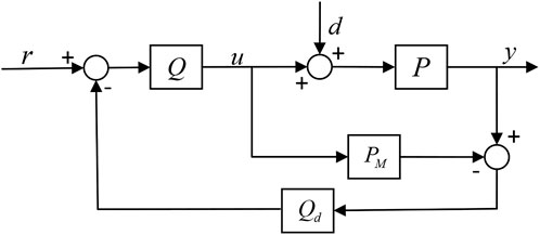
FIGURE 3. Block diagram of TDF-IMC.

We can divide the design process of the TDF-IMC controller into the following steps (Tan and Fu, 2015):

1) Factor the plant model $P_M\left(s\right)$ into two parts:

$\begin{array}{c}{P}_M\left(s\right)=P_{M_{+}}\left(s\right)P_{M_{-}}\left(s\right),\end{array}(20)$

where $P_{M_{+}}\left(s\right)$ is the portion of the model inverted (minimum-phase) and $P_{M_{-}}\left(s\right)$ is the portion of the model not inverted (non-minimum-phase).

2) Design the set-point tracking controller $Q\left(s\right)$ as follows:

$\begin{array}{c}Q\left(s\right)=P_{M_{+}}^{-1}\left(s\right)f\left(s\right),\end{array}(21)$

where $f\left(s\right)$ is a low-pass filter and its expression is given as follows:

$\begin{array}{c}f\left(s\right)=\frac{1}{{\left(\lambda s+1\right)}^n}\end{array}.(22)$

Here, $\lambda$ is the filter parameter, and $n$ is the relative degree of $P_{M_{+}}\left(s\right)$.

3) The disturbance rejection controller $Q_d\left(s\right)$ is designed as follows:

$\begin{array}{c}{Q}_d\left(s\right)=\frac{{\alpha }_m{s}^m+\cdots +{\alpha }_{1}s+1}{{\left({\lambda }_{d}s+1\right)}^{r_d}}\end{array},(23)$

where $m$ is the number of poles of $P_M\left(s\right)$ such that $Q_d\left(s\right)$ needs to cancel the disturbance rejection filter $\frac{1}{{\left({\lambda }_{d}s+1\right)}^{r_d}}$ with order $r_d\ge m$, and ${\lambda }_d$ is a tuning parameter for obtaining a better disturbance-rejecting performance. The poles $p_1\cdots p_m$ of $P_M\left(s\right)$ can be canceled by the zeros ${\alpha }_1\cdots {\alpha }_m$ of $Q_d\left(s\right)$, i.e., ${\alpha }_1\cdots {\alpha }_m$ should satisfy the following:

$\begin{array}{c}{\left.\left(1-P_M\left(s\right)Q\left(s\right)Q_d\left(s\right)\right)\right|}_{s=p_1\cdots p_m}=0.\end{array}(24)$

The corresponding transfer function of the IMC controller is as follows:

$\begin{array}{c}{K}_{IMC}\left(s\right)=\frac{Q\left(s\right)Q_d\left(s\right)}{1-P_M\left(s\right)Q\left(s\right)Q_d\left(s\right)}\end{array}.(25)$

3.2 The IMC controller design for the SOPDT system

By designing the IMC controller, we can get the controller gain of SS-${PIDD}^2$. So consider the general form of SOPDT systems as follows:

$\begin{array}{c}{P}_M\left(s\right)=\frac{k}{T^2{s}^2+2T\xi s+1}{e}^{-\tau s}\end{array}(26)$

The controllers $Q\left(s\right)$ and $Q_d\left(s\right)$ for Eq. 26 are as follows:

$\begin{array}{c}Q\left(s\right)=\frac{T^2{s}^2+2T\xi s+1}{k{\left(\lambda s+1\right)}^2}\end{array}(27)$

$\begin{array}{c}{Q}_d\left(s\right)=\frac{{\alpha }_2{s}^2+{\alpha }_{1}s+1}{{\left({\lambda }_{d}s+1\right)}^3}\end{array}(28)$

Here, the order of the disturbance rejection filter $r_d$ is chosen as 3, and ${\alpha }_1$ and ${\alpha }_2$ meet Eq. 24.

From the aforementioned derivation, the final form of Eq. 25 is given as follows:

$\begin{array}{c}{K}_{IMC}\left(s\right)=\frac{1}{k}\frac{(T^2{s}^2+2T\xi s+1)({\alpha }_2{s}^2+{\alpha }_{1}s+1)}{{\left(\lambda s+1\right)}^2{\left({\lambda }_{d}s+1\right)}^3-{\left({\alpha }_2{s}^2+{\alpha }_{1}s+1\right)e}^{-\tau s}}\end{array}.(29)$

From the aforementioned analysis, we can cancel the roots of $T^2{s}^2+2T\xi s+1$. To obtain a finite-dimensional controller, we take the first-order Pade approximation technique (Horn et al., 1996; Shamsuzzoha and Lee, 2008) to approximate the pure delay.

$\begin{array}{c}{e}^{-\tau s}=\frac{1-\frac{\tau }{2}s}{1+\frac{\tau }{2}s}\end{array}.(30)$

Then, the simplified form of Eq. 29 becomes

$\begin{array}{c}{K}_{IMC}\left(s\right)=\frac{1}{k}\frac{\left(1+\frac{\tau }{2}s\right)\left({\alpha }_2{s}^2+{\alpha }_{1}s+1\right)}{s\left(a_3{s}^3+{a_{2}s}^2{+a}_{1}s+1\right)}=\frac{p_3{s}^3+p_2{s}^2+p_{1}s+p_0}{s\left(q_3{s}^3+q_2{s}^2+q_{1}s+q_0\right)}\end{array},(31)$

where the expression of $p_0,\cdots ,p_3$ and $q_0,\cdots ,q_3$ can be obtained as follows:

$\begin{array}{c}{p}_0=1,p_1=\frac{\tau }{2}+{\alpha }_1,{p_2=\frac{\tau }{2}{\alpha }_1+{\alpha }_2,p}_3=\frac{\tau }{2}{\alpha }_2,\end{array}(32)$

$\begin{array}{c}\begin{array}{c}{q}_0=2\lambda +3{\lambda }_d+{\alpha }_1+\tau ,\\ q_1=\frac{{\alpha }_1}{2}\tau -{\alpha }_2+6\lambda {\lambda }_d+\left(2\lambda +3{\lambda }_d\right)\frac{\tau }{2}+{\lambda }^2+3{\lambda }_d^2-2T\xi q_0,\\ q_2=\frac{\frac{{\left(3{\lambda }^2{\lambda }_d^2+2\lambda {\lambda }_d^3\right)}^2}{2}+{\lambda }^2{\lambda }_d^3-2T\xi q_3}{T^2},q_3=\frac{{\lambda }^2{\lambda }_d^3}{2T^2}\tau .\end{array}\end{array}(33)$

3.3 Specific approximate processes with the state-space ${\mathit{P}\mathit{I}\mathit{D}\mathit{D}}^{\mathbf{2}}$

This subsection focuses on how to attain the parameters of SS-${PIDD}^2$ through IMC. For simplicity, the observer gain ${\overline{L}}_o$ in Eq. 16 can be tuned via the bandwidth idea (Gao, 2003), i.e., the poles of ${\overline{A}}_e-{\overline{L}}_o{\overline{C}}_e$ in Eq. 14 are placed at the same location $-{\overline{\omega }}_o$, and then,

$\begin{array}{c}{\overline{\beta }}_1={{\overline{\omega }}_o}^3,{\overline{\beta }}_2=3{{\overline{\omega }}_o}^2,{\overline{\beta }}_3=3{\overline{\omega }}_o.\end{array}(34)$

According to the aforementioned Eq. 19, the transfer function form of SS-${PIDD}^2$ is as follows:

$\begin{array}{c}\begin{array}{c}{K}_c\left(s\right)={\overline{K}}_o{\left(sI-{\overline{A}}_e+{\overline{B}}_e{\overline{K}}_o+{\overline{L}}_o{\overline{C}}_e\right)}^{-1}{\overline{L}}_o\\ =\frac{c_3{s}^3+c_2{s}^2+c_{1}s+c_0}{s\left(e_3{s}^3+e_2{s}^2+e_{1}s+e_0\right)},\end{array}\end{array}(35)$

where

$\begin{array}{c}\left[\begin{array}{c}{c}_3\\ c_2\\ c_1\\ c_0\end{array}\right]=\left[\begin{array}{cccc}{\overline{\beta }}_1& {\overline{\beta }}_2& {\overline{\beta }}_3& 1\\ 0& {\overline{\beta }}_1& {\overline{\beta }}_2& {\overline{\beta }}_3\\ 0& 0& {\overline{\beta }}_1& {\overline{\beta }}_2\\ 0& 0& 0& {\overline{\beta }}_1\end{array}\right]\left[\begin{array}{c}{K}_{dd}\\ K_d\\ K_p\\ K_i\end{array}\right]\end{array},(36)$

$\begin{array}{c}\left[\begin{array}{c}{e}_3\\ e_2\\ e_1\\ e_0\end{array}\right]=\left[\begin{array}{cccc}1& 0& 0& 0\\ {\overline{\beta }}_3& 1& 0& 0\\ {\overline{\beta }}_2& {\overline{\beta }}_3& 1& 0\\ {\overline{\beta }}_1& {\overline{\beta }}_2& {\overline{\beta }}_3& 1\end{array}\right]\left[\begin{array}{c}1\\ K_{dd}\\ K_d\\ K_p\end{array}\right]\end{array}.(37)$

To make the SS-${PIDD}^2$ controller achieve the same control performance as the IMC controller, suppose Eq. 31 and 35 have the same zeros, i.e.,

$\begin{array}{c}\left[\begin{array}{c}{c}_3\\ c_2\\ c_1\\ c_0\end{array}\right]=\alpha \left[\begin{array}{c}{p}_3\\ p_2\\ p_1\\ p_0\end{array}\right],\end{array}(38)$

where $\alpha$ is an optional constant. According to Eq. 36, we have the following:

$\begin{array}{c}\left[\begin{array}{c}{c}_3\\ c_2\\ c_1\\ c_0\end{array}\right]=\left[\begin{array}{cccc}{\overline{\beta }}_1& {\overline{\beta }}_2& {\overline{\beta }}_3& 1\\ 0& {\overline{\beta }}_1& {\overline{\beta }}_2& {\overline{\beta }}_3\\ 0& 0& {\overline{\beta }}_1& {\overline{\beta }}_2\\ 0& 0& 0& {\overline{\beta }}_1\end{array}\right]\left[\begin{array}{c}{K}_{dd}\\ K_d\\ K_p\\ K_i\end{array}\right]=\alpha \left[\begin{array}{c}{p}_3\\ p_2\\ p_1\\ p_0\end{array}\right].\end{array}(39)$

Thus, the controller gain of SS-${PIDD}^2$ can be obtained as follows:

$\begin{array}{c}\begin{array}{c}\left[\begin{array}{c}{K}_{dd}\\ K_d\\ K_p\\ K_i\end{array}\right]=\alpha {\left[\begin{array}{cccc}{\overline{\beta }}_1& {\overline{\beta }}_2& {\overline{\beta }}_3& 1\\ 0& {\overline{\beta }}_1& {\overline{\beta }}_2& {\overline{\beta }}_3\\ 0& 0& {\overline{\beta }}_1& {\overline{\beta }}_2\\ 0& 0& 0& {\overline{\beta }}_1\end{array}\right]}^{-1}\left[\begin{array}{c}{p}_3\\ p_2\\ p_1\\ p_0\end{array}\right]\\ =\alpha \left[\begin{array}{cccc}\frac{1}{{\overline{\beta }}_1}& -\frac{{\overline{\beta }}_2}{{{\overline{\beta }}_1}^2}& \frac{{{\overline{\beta }}_2}^2-{\overline{\beta }}_1{\overline{\beta }}_3}{{{\overline{\beta }}_1}^3}& \frac{2{\overline{\beta }}_1{\overline{\beta }}_2{\overline{\beta }}_3-{{\overline{\beta }}_2}^3-{{\overline{\beta }}_1}^2}{{{\overline{\beta }}_1}^4}\\ 0& \frac{1}{{\overline{\beta }}_1}& -\frac{{\overline{\beta }}_2}{{{\overline{\beta }}_1}^2}& \frac{{{\overline{\beta }}_2}^2-{\overline{\beta }}_1{\overline{\beta }}_3}{{{\overline{\beta }}_1}^3}\\ 0& 0& \frac{1}{{\overline{\beta }}_1}& -\frac{{\overline{\beta }}_2}{{{\overline{\beta }}_1}^2}\\ 0& 0& 0& \frac{1}{{\overline{\beta }}_1}\end{array}\right]\left[\begin{array}{c}{p}_3\\ p_2\\ p_1\\ p_0\end{array}\right]\end{array}\\ \begin{array}{c}=\alpha \frac{1}{{\overline{\beta }}_1}{p}_3-\alpha \frac{{\overline{\beta }}_2}{{{\overline{\beta }}_1}^2}{p}_2+\alpha \frac{{{\overline{\beta }}_2}^2-{\overline{\beta }}_1{\overline{\beta }}_3}{{{\overline{\beta }}_1}^3}{p}_1+\alpha \frac{2{\overline{\beta }}_1{\overline{\beta }}_2{\overline{\beta }}_3-{{\overline{\beta }}_2}^3-{{\overline{\beta }}_1}^2}{{{\overline{\beta }}_1}^4}{p}_0\\ =\alpha \frac{1}{{\overline{\beta }}_1}{p}_2-\alpha \frac{{\overline{\beta }}_2}{{{\overline{\beta }}_1}^2}{p}_1+\alpha \frac{{{\overline{\beta }}_2}^2-{\overline{\beta }}_1{\overline{\beta }}_3}{{{\overline{\beta }}_1}^3}{p}_0\\ \begin{array}{c}=\alpha \frac{1}{{\overline{\beta }}_1}{p}_1-\alpha \frac{{\overline{\beta }}_2}{{{\overline{\beta }}_1}^2}{p}_0\\ =\frac{1}{{\overline{\beta }}_1}{p}_0.\end{array}\end{array}\end{array}(40)$

The final parameters of SS-${PIDD}^2$ can be obtained by substituting Eqs 32 and 34 into Eq. 40. The important thing to note here is to make $\alpha$ as large as possible so that ${\overline{\omega }}_o$ is a positive real-number.

3.4 Tuning rules for SOPDT systems

The performance of the IMC controller is decided by the parameters $\lambda$ and ${\lambda }_d$. Nevertheless, previous studies of the IMC have not dealt with how to obtain the appropriate value of these two parameters. In other words, there is no specific approach to choose the value of $\lambda$ and ${\lambda }_d$. Hence, the core idea of this subsection is to get optimized values of $\lambda$ and ${\lambda }_d$. The optimal values of $\lambda$ and ${\lambda }_d$ are those that give the minimum (integral of the time squared error) ITSE with certain robustness, and then, we can get the transfer function of the equivalent IMC controller. Thus, according to Section 3.3, we can obtain the parameters ($K_p$; $K_i$; $K_d$; $K_{dd}$; ${\omega }_o$) of the SS-${PIDD}^2$ controller. The specific flow chart of the derivation process is shown in Figure 4.

FIGURE 4

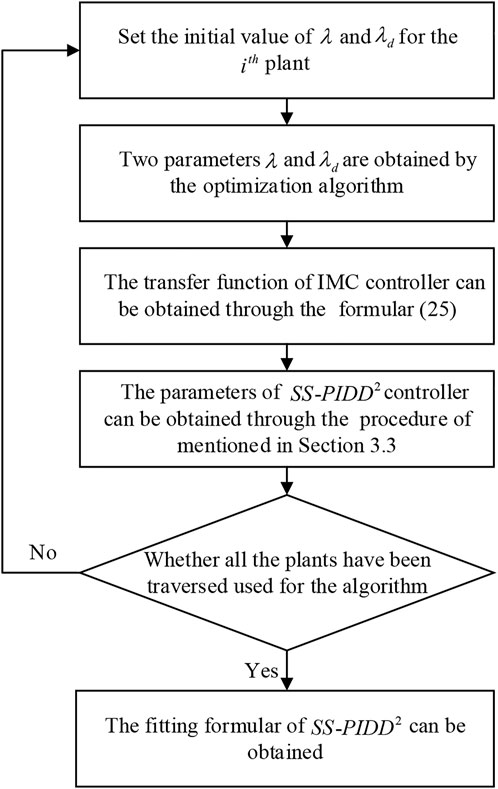
FIGURE 4. Flow chart of the derivation of the tuning formula.

In the process of calculating the parameters of SS-${PIDD}^2$, as mentioned in Figure 4, we notice that the parameters of the SS-${PIDD}^2$ controller exhibit different properties for $\tau /T\le 2.5$ and $\tau /T>2.5$; consequently, we set the parameters in the two cases, respectively.

To describe the detailed derivation process of the tuning formula, suppose $\tau /T\le 2.5$ and consider a normalized SOPDT system, then

$\begin{array}{c}G\left(s\right)=\frac{1}{s^2+2\times 0.2\times s+1}{e}^{-\overline{\tau }s}\end{array},(41)$

where $\overline{\tau }$ varies from .5 to 2.5 with an appropriate step. A set of parameters of SS-${PIDD}^2$ $K_p$, $K_i$, $K_d$, $K_{dd}$, and ${\omega }_o$ can be obtained through the process in Figure 4. The fitting curves of parameters of the SS-${PIDD}^2$ are shown in Figure 5.

FIGURE 5

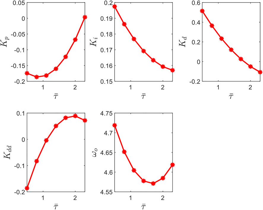
FIGURE 5. Fitting curves of parameters of SS-${\mathit{P}\mathit{I}\mathit{D}\mathit{D}}^{\mathbf{2}}$.

The corresponding function expressions are given in Eq. 42:

$\begin{array}{c}\begin{array}{c} {\overline{K}}_p=0.0924{\overline{\tau }}^2-0.1599\overline{\tau }-0.1176,\\ {\overline{K}}_i=0.0099{\overline{\tau }}^2-0.0502\overline{\tau }+0.2201,\\ {\overline{K}}_d=0.1027{\overline{\tau }}^2-0.6332\overline{\tau }+0.8056,\\ {\overline{K}}_{dd}=-0.1334{\overline{\tau }}^2+0.5169\overline{\tau }-0.4112,\\ {\overline{\omega }}_o=0.1125{\overline{\tau }}^2-0.3707\overline{\tau }+4.8762.\end{array}\end{array}(42)$

So we can rewrite Eq. 42 as follows:

$\begin{array}{c}\begin{array}{c}{\overline{K}}_p=A_1{\overline{\tau }}^2+A_2\overline{\tau }+A_{3,}\\ {\overline{K}}_i=B_1{\overline{\tau }}^2+B_2\overline{\tau }+B_3,\\ {\overline{K}}_d=C_1{\overline{\tau }}^2+C_2\overline{\tau }+C_3,\\ {\overline{K}}_{dd}=D_1{\overline{\tau }}^2+D_2\overline{\tau }+D_3,\\ {\overline{\omega }}_o=E_1{\overline{\tau }}^2+E_2\overline{\tau }+E_3.\end{array}\end{array}(43)$

When $\xi =0.1;0.3;0.4;0.5;0.6;0.7$, the corresponding fitting curves of $K_p$, $K_i$, $K_d$, $K_{dd}$, ${\omega }_o,$ and $\xi$ are obtained, as shown in Figure 6. The fitting formulae are given in Eq. 44:3

$\begin{array}{c}\begin{array}{c}{A}_1=0.3{\xi }^2-0.4434\xi +0.1691,\\ A_2=-1.102{\xi }^2+1.354\xi -0.3866,\\ A_3=0.7656{\xi }^2+0.2038\xi -0.189,\\ B_1=0.02727{\xi }^2-0.01403\xi +0.01164,\\ B_2=-0.1443{\xi }^2+0.02041\xi -0.04854,\\ B_3=0.313\xi +0.1575,\\ C_1=-0.2909{\xi }^2+0.06036\xi +0.1023,\\ C_2=1.258\xi -0.8848,\\ C_3=-1.187\xi +1.043,\\ D_1=-0.3103{\xi }^2+0.4958\xi -0.2201,\\ D_2=0.8436{\xi }^2-1.519\xi +0.787,\\ D_3=-0.5418{\xi }^2+0.9786\xi -0.5852,\\ E_1=0.4148{\xi }^2-0.5456\xi +0.205,\\ E_2=-3.695{\xi }^{-0.04876}+3.626,\\ E_3=-56.83{\xi }^{0.00182}+61.54,\end{array}\end{array}(44)$

where $\overline{\tau }$ varies from 2.5 to 5 with an appropriate step. A set of parameters of SS-${PIDD}^2$ $K_p$, $K_i$, $K_d$, $K_{dd}$, and ${\omega }_o$ can be obtained through the process in Figure 4. The fitting curves of parameters of SS-${PIDD}^2$ are shown in Figures 7, 9.

FIGURE 6

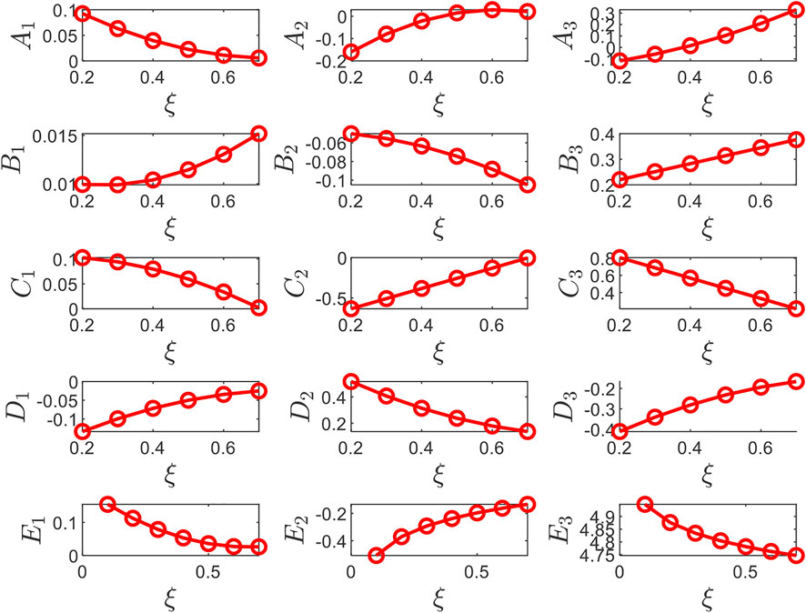
FIGURE 6. Fitting curves of ${\mathit{K}}_{\mathit{p}}$, ${\mathit{K}}_{\mathit{i}}$, ${\mathit{K}}_{\mathit{d}}$, ${\mathit{K}}_{\mathit{d}\mathit{d}}$, ${\mathit{\omega }}_{\mathit{o}},$ and $\mathit{\xi }$.

FIGURE 7

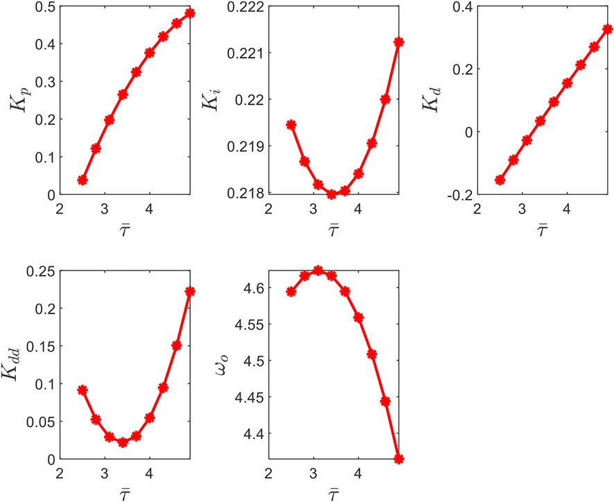
FIGURE 7. Fitting curves of parameters of SS-${\mathit{P}\mathit{I}\mathit{D}\mathit{D}}^{\mathbf{2}}$.

The corresponding function expressions are given in Eq. 45:

$\begin{array}{c}\begin{array}{c} {\overline{K}}_p=-0.0452{\overline{\tau }}^2+0.5190\overline{\tau }-0.9770,\\ {\overline{K}}_i=0.0016{\overline{\tau }}^2-0.0111\overline{\tau }+0.2372,\\ {\overline{K}}_d=-0.0059{\overline{\tau }}^2+0.2437\overline{\tau }-0.7264,\\ {\overline{K}}_{dd}=0.0878{\overline{\tau }}^2-0.5952\overline{\tau }+1.0306,\\ {\overline{\omega }}_o=-0.0800{\overline{\tau }}^2+0.4963\overline{\tau }+3.8536.\end{array}\end{array}(45)$

Similar to Eq. 44, we can obtain the following:

$\begin{array}{c}\begin{array}{c}{A}_1=-0.0909{\xi }^2+0.1645\xi -0.07444,\\ A_2=1.405{\xi }^2-2.175\xi +0.8978,\\ A_3=-3.166{\xi }^2+5.363\xi -1.923,\\ B_1=0.02167{\xi }^2-0.01522\xi +0.003777,\\ B_2=-0.09188{\xi }^2-0.001259\xi -0.007188,\\ B_3=0.3004{\xi }^2+0.007393\xi +0.1756,\\ C_1=7.843e-09{\xi }^{-6.822}-0.006375,\\ C_2=0.6736{\xi }^2-1.011\xi +0.419,\\ C_3=2.95{\xi }^2+4.443\xi -1.497,\\ D_1=0.04845{\xi }^{-0.7432}-0.07248,\\ D_2=-0.286{\xi }^{-0.8213}+0.4774,\\ D_3=0.4976{\xi }^{-0.8112}-0.8055,\\ E_1=-0.02299{\xi }^{-1.035}+0.04166,\\ E_2=0.1223{\xi }^{-1.143}-0.2734,\\ E_3=-0.1418{\xi }^{-1.264}+4.938.\end{array}\end{array}(46)$

When $\xi =0.1;0.3;0.4;0.5;0.6;0.7$, the corresponding fitting curves of $K_p$, $K_i$, $K_d$, $K_{dd}$, ${\omega }_o,$ and $\xi$ are obtained, as shown in Figures 8, 10.

FIGURE 8

FIGURE 8. Fitting curves of ${\mathit{K}}_{\mathit{p}}$, ${\mathit{K}}_{\mathit{i}}$, ${\mathit{K}}_{\mathit{d}}$, ${\mathit{K}}_{\mathit{d}\mathit{d}}$, ${\mathit{\omega }}_{\mathit{o}},$ and $\mathit{\xi }$.

In practice, the relationship between ${\overline{K}}_p$, ${\overline{K}}_i$, ${\overline{K}}_d$, ${\overline{K}}_{dd}$, and ${\overline{\omega }}_o$ of SS-${PIDD}^2$ for the normalized SOPDT model in Eq. 41 and $K_p$, $K_i$, $K_d$, $K_{dd}$, and ${\omega }_o$ of SS-${PIDD}^2$ for the general SOPDT model in Eq. 26is described in the following (Zhang et al., 2019):

$\begin{array}{c}{K}_p=\frac{{\overline{K}}_p}{k},K_i=\frac{{\overline{K}}_i}{Tk},K_d=\frac{{\overline{K}}_{d}T}{k},K_{dd}=\frac{{\overline{K}}_{dd}{T}^2}{k},{\omega }_o=\frac{{\overline{\omega }}_o}{T}\end{array}.(47)$

As a result, combining Eqs 43−47, we can obtain the following tuning formula of SS-${PIDD}^2$ for the SOPDT system:

$\begin{array}{c}\begin{array}{c}{K}_p=\frac{\left(0.3{\xi }^2-0.4434\xi +0.1691\right){\tau }^2}{{kT}^2}+\frac{\left(-1.102{\xi }^2+1.354\xi -0.3866\right)\tau }{kT}\\ +\frac{0.7656{\xi }^2+0.2038\xi -0.189}{k},\\ K_i=\frac{\left(0.02727{\xi }^2-0.01403\xi +0.01164\right){\tau }^2}{k{T}^3}+\frac{\left(-0.1443{\xi }^2+0.02041\xi -0.04854\right)\tau }{k{T}^2}\\ +\frac{0.313\xi +0.1575}{kT},\\ K_d=\frac{\left(-0.2909{\xi }^2+0.06036\xi +0.1023\right){\tau }^2}{kT}+\frac{\left(1.258\xi -0.8848\right)\tau }{k}+\frac{\left(-1.187\xi +1.043\right)T}{k},\\ K_{dd}=\frac{\left(-0.3103{\xi }^2+0.4958\xi -0.2201\right){\tau }^2}{k}+\frac{\left(0.8436{\xi }^2-1.519\xi +0.787\right)\tau T}{k}\\ +\frac{\left(-0.5418{\xi }^2+0.9786\xi -0.5852\right)T^2}{k},\\ {\omega }_o=\frac{\left(0.4148{\xi }^2-0.5456\xi +0.205\right){\tau }^2}{T^3}+\frac{\left(-3.695{\xi }^{-0.04876}+3.626\right)\tau }{T^2}\\ +\frac{-56.83{\xi }^{0.00182}+61.54}{T}.\end{array}\end{array}(48)$

Similarly, using the same process, we can obtain the tuning formula when $\tau /T>2.5$ as follows:

$\begin{array}{c}\begin{array}{c}{K}_p=\frac{\left(-0.0909{\xi }^2+0.1645\xi -0.07444\right){\tau }^2}{{kT}^2}+\frac{\left(1.405{\xi }^2-2.175\xi +0.8978\right)\tau }{kT}\\ +\frac{-3.166{\xi }^2+5.363\xi -1.923}{k},\\ K_i=\frac{\left(0.02167{\xi }^2-0.01522\xi +0.003777\right){\tau }^2}{k{T}^3}+\frac{\left(-0.09188{\xi }^2-0.001259\xi -0.007188\right)\tau }{k{T}^2}\\ +\frac{{0.3004\xi }^2+0.007393\xi +0.1756}{kT},\\ K_d=\frac{\left(7.843e-09{\xi }^{-6.822}-0.006375\right){\tau }^2}{kT}+\frac{\left(0.6736{\xi }^2-1.011\xi +0.419\right)\tau }{k}\\ +\frac{\left(-2.95{\xi }^2+4.443\xi -1.497\right)T}{k},\\ K_{dd}=\frac{\left(0.04845{\xi }^{-0.7432}-0.07248\right){\tau }^2}{k}+\frac{\left(-0.286{\xi }^{-0.8213}+0.4774\right)\tau T}{k}\\ +\frac{\left(0.4976{\xi }^{-0.8112}-0.8055\right)T^2}{k},\\ {\omega }_o=\frac{\left(-0.02299{\xi }^{-1.035}+0.04166\right){\tau }^2}{T^3}+\frac{\left(0.1223{\xi }^{-1.143}-0.2734\right)\tau }{T^2}\\ +\frac{-0.1418{\xi }^{-1.264}+4.938}{T}.\end{array}.\end{array}(49)$

4 Simulation and analyses

This section demonstrates the tuning formula for several examples. In every simulation example, a different control effect has been analyzed and compared with existing methods.

4.1 Simple simulation examples

Simple second-order oscillatory plants with damping ratios $\left(\xi =0.2,\xi =0.4,\xi =0.6\right)$ and delay time $\left(T=1,\tau /T=\mathrm{1,2,3,4}\right)$ are shown in Figures 7–11 (the figures show controller outputs $u\left(t\right)$ within the appropriate range; otherwise, $u\left(t\right)$ for the disturbance response will be too small to be visible in the figure). The parameters and indexes (($ITSE={\int }_0^{\infty }t{e}^2\left(t\right)dt$; $\epsilon :=\underset{\omega }{\mathit{sup}}\left({‖S‖}_{\infty }+{‖T‖}_{\infty }\right)$; ($TV={\sum }_1^{\infty }\left|u_{i+1}\left(t\right)-u_i\left(t\right)\right|$)) are shown in Tables 1–3. The responses for a step reference signal (the amplitude is 1) at $t=0s$ and a step input disturbance signal (the amplitude is .5) are added to these systems at an appropriate time to test the disturbance rejection performance and robustness. Moreover, suppose there is a white noise signal with a variance of $0.001$ added to the output of the plant to test the performance of measurement noise attenuation. From Figures 7–10, we can see that the output responses of the system with $\xi =0.2;0.4$ show large oscillations, which is because the poles of the system are close to the imaginary axis. The responses of the system with $\xi =0.6$ are shown in Figure 11. Compared with the PID controller, the SS-${PIDD}^2$ controller has a faster tracking and disturbance rejection response. Moreover, the SS-${PIDD}^2$ controller has smaller overshooting and fluctuation than the PID controller. In particular, after adding noise, the SS-${PIDD}^2$ controller output response is significantly better than the other two PID methods. Combining figures and tables, we can see that the tuning in Eqs 48, 49 can achieve a better response. Therefore, we can conclude that the proposed formula of SS-${PIDD}^2$ has a better control effect for the SOPDT system.

FIGURE 9

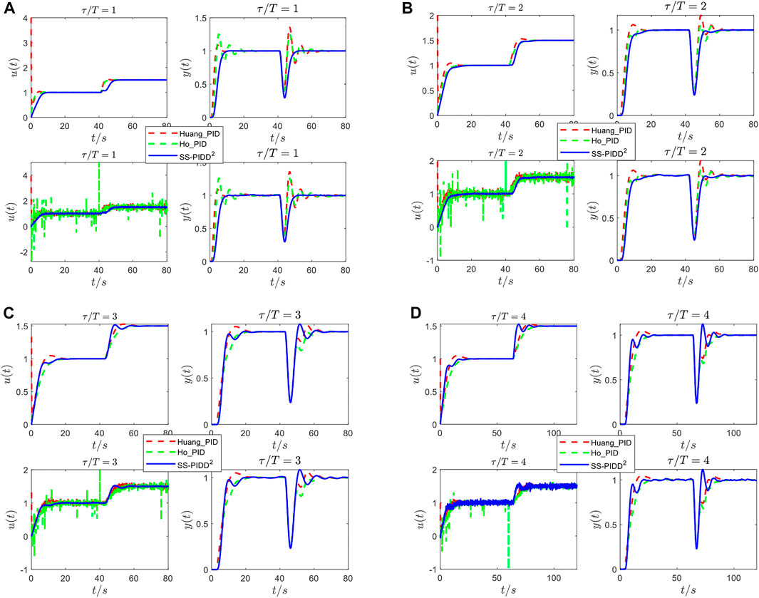
FIGURE 9. Responses of the SOPDT system with ξ = .2 under different controllers: controller output responses without noise [the top left of (A–D)]; system output responses without noise [the top right of (A–D)]; controller output responses with noise [the bottom left of (A–D)]; (B) system output responses with noise [the bottom right of (A–D)].

FIGURE 10

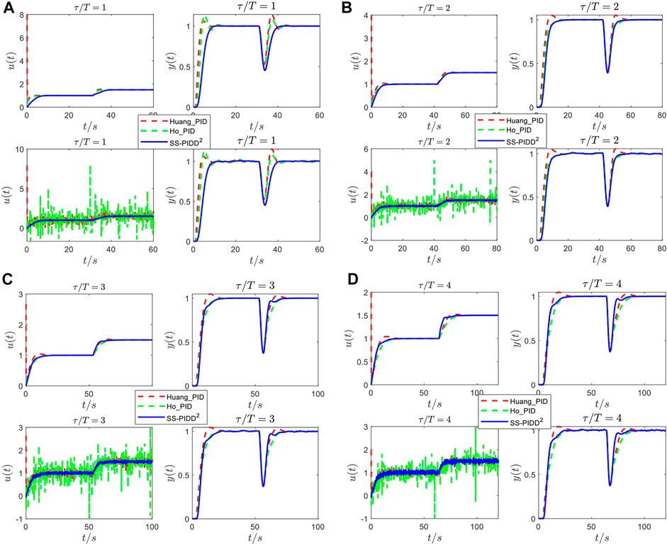
FIGURE 10. Responses of the SOPDT system with ξ = 0.4 under different controllers: controller output responses without noise [the top left of (A–D)]; system output responses without noise [the top right of (A–D)]; controller output responses with noise [the bottom left of (A–D)]; (B) system output responses with noise [the bottom right of (A–D)].

FIGURE 11

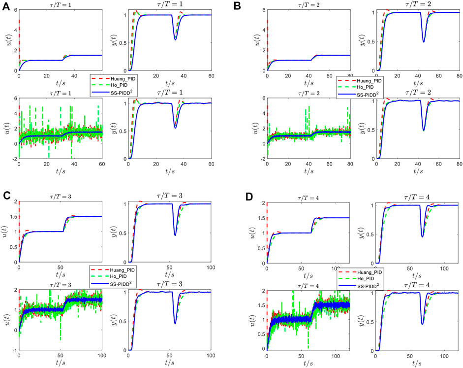
FIGURE 11. Responses of the SOPDT system with ξ = 0.6 under different controllers: controller output responses without noise [the top left of (A–D)]; system output responses without noise [the top right of (A–D)]; controller output responses with noise [the bottom left of (A–D)]; (B) system output responses with noise [the bottom right of (A–D)].

TABLE 1

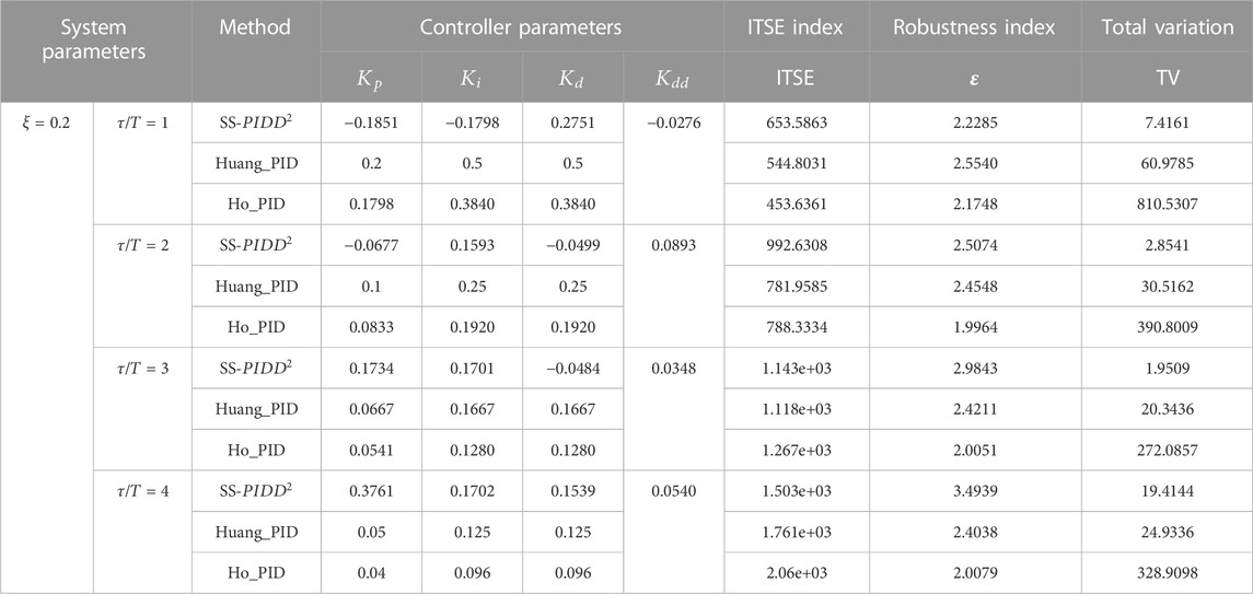
TABLE 1. Parameters of the SS-${\mathit{P}\mathit{I}\mathit{D}\mathit{D}}^{\mathbf{2}}$ and PID controllers for $\mathit{\xi }=\mathbf{0.2}$.

TABLE 2

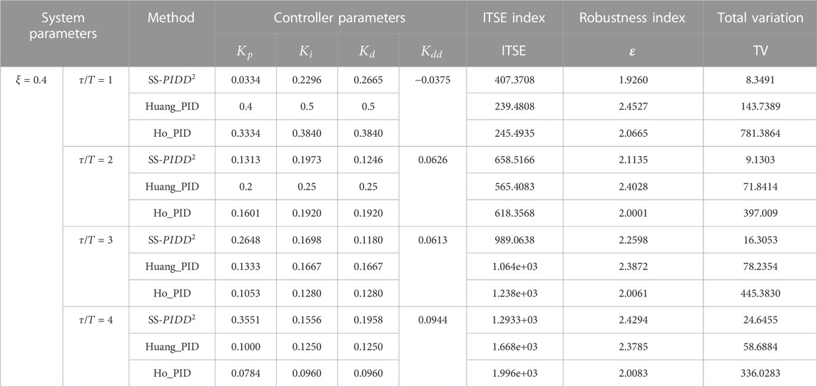
TABLE 2. Parameters of the SS-${\mathit{P}\mathit{I}\mathit{D}\mathit{D}}^{\mathbf{2}}$ and PID controllers for $\mathit{\xi }=\mathbf{0.4}$.

TABLE 3

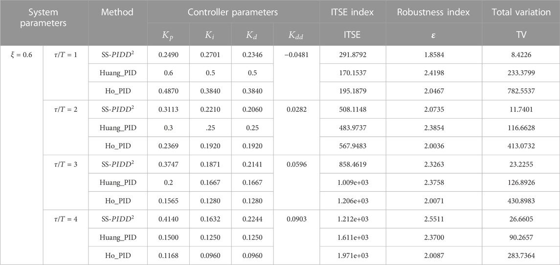
TABLE 3. Parameters of the SS-${\mathit{P}\mathit{I}\mathit{D}\mathit{D}}^{\mathbf{2}}$ and PID controllers for $\mathit{\xi }=\mathbf{0.6}$.

Remark: 1) Robustness is the property that a control system maintains for some other performance under certain (structure and size) parameter perturbations.

$\begin{array}{c}{M}_s={‖S‖}_{\infty }=\underset{\omega }{\mathit{max}}\left|\frac{1}{1+L\left(j\omega \right)}\right|,\\ M_t={‖T‖}_{\infty }=\underset{\omega }{\mathit{max}}\left|\frac{L\left(j\omega \right)}{1+L\left(j\omega \right)}\right|,\\ \epsilon :=\underset{\omega }{\mathit{sup}}\left({‖S‖}_{\infty }+{‖T‖}_{\infty }\right),\end{array}$

where $L\left(s\right)$ is the open-loop transfer function of the system, $M_s$ and $M_t$ are maximum sensitivities, $S\left(s\right)$ and $T\left(s\right)$ are sensitivity functions, and $\epsilon$ represents the robustness of the system.

2) ITSE is the integral of the time squared error. $ITSE={\int }_0^{\infty }t{e}^2\left(t\right)dt$. $e\left(t\right)=r\left(t\right)-y\left(t\right)$ is the difference between the reference input signal and output signal of the system.

3) TV is the total variation in the output of the controller. $TV={\sum }_1^{\infty }\left|u_{i+1}\left(t\right)-u_i\left(t\right)\right|$.

4.2 Complex simulation examples

In this subsection, we use three relatively complex oscillatory plants ($G_1$ (Huang et al., 2005), $G_2,$ and $G_3$ (Wang et al., 1999)) to verify the applicability of the proposed Eqs 48 and 49. Dynamic responses of plants are given in Figures 12–14. The controller parameters, systems parameters, and controller performance index are shown in Table 4. It is shown that SS-${PIDD}^2$ and PID have similar disturbance rejection responses; SS-${PIDD}^2$ has a smaller overshoot in the set-point for $G_1$ and set-point tracking responses without the overshoot for $G_2$ and $G_3$.Additionally, the influence of the measurement noise on SS-${PIDD}^2$ is smaller than PID. Significantly, SS-${PIDD}^2$ does not have a satisfactory disturbance rejection performance, compared to the linear active disturbance rejection controller (LADRC) for $G_3$ but has a smaller robustness and TV than LADRC. Generally speaking, the proposed tuning approach has a better control effort and can trade-off between the performance, robustness, and attenuation of the measurement noise.

$\begin{array}{c}{G}_1\left(s\right)=\frac{1}{\left({9s}^2+2.4s+1\right)\left(s+1\right)}{e}^{-2s},\end{array}(50)$

$\begin{array}{c}{G}_2\left(s\right)=\frac{1}{\left(s^2+2s+3\right)\left(s+3\right)}{e}^{-0.3s},\end{array}(51)$

$\begin{array}{c}{G}_3\left(s\right)=\frac{1}{\left(s^2+s+1\right){\left(s+2\right)}^2}{e}^{-0.1s}.\end{array}(52)$

FIGURE 12

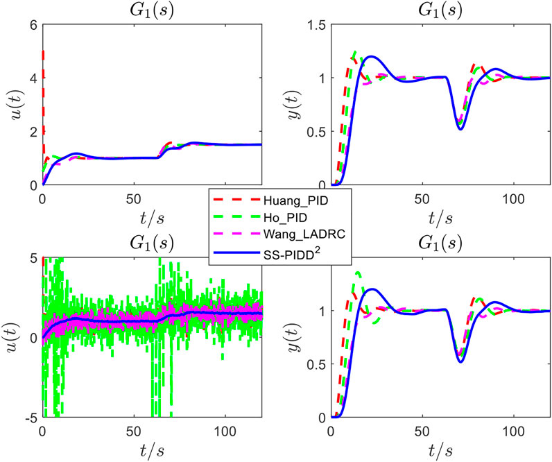
FIGURE 12. Responses of ${\mathit{G}}_{\mathbf{1}}\left(\mathit{s}\right)$: controller output responses without noise (the top left); system output responses without noise (the top right); controller output responses with noise (the bottom left); system output responses with noise (the bottom right).

FIGURE 13

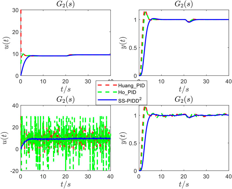
FIGURE 13. Responses of ${\mathit{G}}_{\mathbf{2}}\left(\mathit{s}\right)$: controller output responses without noise (the top left); system output responses without noise (the top right); controller output responses with noise (the bottom left); system output responses with noise (the bottom right).

FIGURE 14

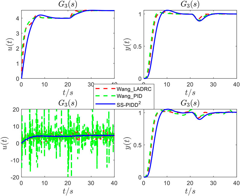
FIGURE 14. Responses of ${\mathit{G}}_{\mathbf{3}}\left(\mathit{s}\right)$: controller output responses without noise (the top left); system output responses without noise (the top right); controller output responses with noise (the bottom left); system output responses with noise (the bottom right).

TABLE 4

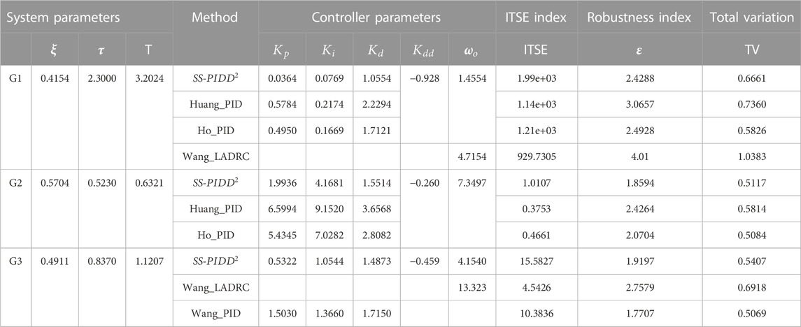
TABLE 4. Parameters of the SS-${\mathit{P}\mathit{I}\mathit{D}\mathit{D}}^{\mathbf{2}}$ and PID controllers for (50)–(52).

4.3 Practical system simulations

Consider the load frequency control system as a typical oscillatory SOPDT system. Additionally, the system’s uncertainty and control complexity will rise due to communication delays. Therefore, the proposed SS-${PIDD}^2$ controller is applied to the LFC system with communication delays in this section to test its effectiveness.

To illustrate the issue, we take the one-area non-reheat system as an example (Fu and Tan, 2018). The transfer function model of the LFC system is shown in Figure 15. The transfer function of each part is as follows:

$\begin{array}{c}{G}_g\left(s\right)=\frac{1}{0.08s+1},G_t\left(s\right)=\frac{1}{0.3s+1},G_p\left(s\right)=\frac{120}{20s+1}\end{array}(53)$

and

$\begin{array}{c}R=2.4,{\tau }_d+{\tau }_h=1.5.\end{array}(54)$

FIGURE 15

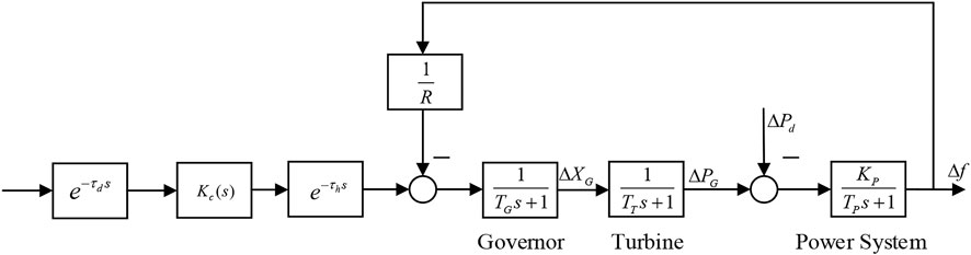
FIGURE 15. Transfer function model of the load frequency control system.

The system parameters are as follows (Fu and Tan, 2018):

$\begin{array}{c}k=2.3568,\xi =0.4665,T=0.3700,\tau =1.5\end{array}.(55)$

Suppose there is a disturbance of $∆P_d=0.01pu$ added to the output of the controller. From Figure 16, we can conclude that the proposed controller has a faster response speed and better disturbance rejection performance.

FIGURE 16

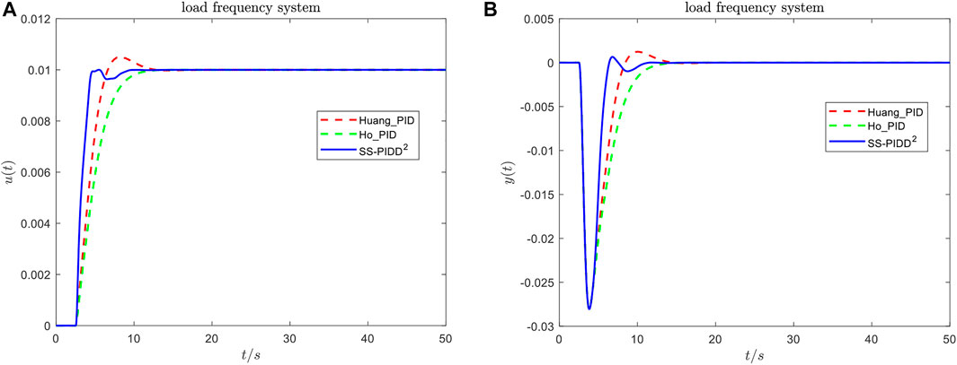
FIGURE 16. System responses under different controllers: (A) controller output responses and (B) system output responses.

5 Conclusion

The purpose of this paper was to provide a tuning formula of the ${PIDD}^2$ controller for oscillatory systems with time delays. The ideal ${PIDD}^2$ controller was implemented via the state-space form, which takes a cascaded integral model to estimate the output of the controlled plant and its derivatives; accordingly, it retains the plant-independence property of the traditional PID. A total of two state-space ${PIDD}^2$ tuning formulas were attained for SOPDT systems with time delays, and the parameters of ${PIDD}^2$ can be determined by approximating an IMC controller. The proposed formulas are applied to a wide range of plants. In addition, further simulation analysis of ${PIDD}^2$ was used to test the effectiveness of the proposed tuning formula. Compared with the PID controller, the state-space ${PIDD}^2$ controller has roll-offs at high frequencies; thus, it is more insensitive to measurement noises.

The empirical findings in this study provide a new understanding of ${PIDD}^2$ controllers. Future research will be devoted to the control of ${PIDD}^2$ oscillatory systems with zeros.

Data availability statement

The raw data supporting the conclusion of this article will be made available by the authors, without undue reservation.

Author contributions

HX, HG, and TW contributed to the conceptualization and methodology. HX wrote the first draft of the manuscript. All authors contributed to manuscript revision and read and approved the submitted version.

Conflict of interest

The authors declare that the research was conducted in the absence of any commercial or financial relationships that could be construed as a potential conflict of interest.

Publisher’s note

All claims expressed in this article are solely those of the authors and do not necessarily represent those of their affiliated organizations, or those of the publisher, the editors, and the reviewers. Any product that may be evaluated in this article, or claim that may be made by its manufacturer, is not guaranteed or endorsed by the publisher.

References

Basilio, J. C., and Matos, S. (2002). Design of PI and PID controllers with transient performance specification. IEEE Trans. Educ. 45, 364–370. doi:10.1109/te.2002.804399

CrossRef Full Text | Google Scholar

Borase, R. P., Maghade, D. K., Sondkar, S. Y., and Pawar, S. N. (2021). A review of PID control, tuning methods and applications. Int. J. Dynam. Control 9, 818–827. doi:10.1007/s40435-020-00665-4

CrossRef Full Text | Google Scholar

Chan, Y. F., Moallem, M., and Wang, W. (2007). Design and implementation of modular FPGA-based PID controllers. IEEE Trans. Ind. Electron. 54, 1898–1906. doi:10.1109/tie.2007.898283

CrossRef Full Text | Google Scholar

Chao, C.-T., Sutarna, N., Chiou, J.-S., and Wang, C.-J. (2019). An optimal fuzzy PID controller design based on conventional PID control and nonlinear factors. Appl. Sci. 9, 1224. doi:10.3390/app9061224

CrossRef Full Text | Google Scholar

Chatterjee, S., Dalel, M. A., and Palavalasa, M., 2019. “Design of PID plus second order derivative controller for automatic voltage regulator using whale optimizatio algorithm,” in 2019 3rd International Conference on Recent Developments in Control, Automation & Power Engineering (RDCAPE), NOIDA, India, 10-11 October 2019 (IEEE), 574–579.Presented at the 2019 3rd International Conference on Recent Developments in Control, Automation & Power Engineering (RDCAPE).

CrossRef Full Text | Google Scholar

Chevalier, A., Francis, C., Copot, C., Ionescu, C. M., and De Keyser, R. (2019). Fractional-order PID design: Towards transition from state-of-art to state-of-use. ISA Trans. 84, 178–186. doi:10.1016/j.isatra.2018.09.017

PubMed Abstract | CrossRef Full Text | Google Scholar

Farooq, Z., Rahman, A., and Lone, S. A. (2021). “Fuzzy and MBO optimized load frequency control of hybrid power system,” in 2021 IEEE 18th India Council International Conference (INDICON). Presented at the 2021 IEEE 18th India Council International Conference (INDICON), Guwahati, India, 19-21 December 2021 (IEEE), 1–6.

CrossRef Full Text | Google Scholar

Fu, C., and Tan, W. (2018). Decentralised load frequency control for power systems with communication delays via active disturbance rejection. IET Generation, Transm. Distribution 12, 1397–1403. doi:10.1049/iet-gtd.2017.0852

CrossRef Full Text | Google Scholar

Gao, Z. (2003). “Scaling and bandwidth-parameterization based controller tuning,” in Proceedings of the 2003 American Control Conference, 2003, Denver, CO, USA, 04-06 June 2003 (IEEE), 4989–4996. Presented at the 2003 American Control Conference.

Google Scholar

Garpinger, O., Hägglund, T., and Åström, K. J. (2014). Performance and robustness trade-offs in PID control. J. Process Control 24, 568–577. doi:10.1016/j.jprocont.2014.02.020

CrossRef Full Text | Google Scholar

Gundes, A. N., and Ozguler, A. B. (2007). PID stabilization of MIMO plants. IEEE Trans. Autom. Contr. 52, 1502–1508. doi:10.1109/tac.2007.902763

CrossRef Full Text | Google Scholar

Halikias, G. D., and Zolotas, A. C. (1999). Optimal design of PID controllers using the QFT method. IEE Proc. - Control Theory Appl. 146, 585–589. doi:10.1049/ip-cta:19990746

CrossRef Full Text | Google Scholar

Horn, I. G., Arulandu, J. R., Gombas, C. J., VanAntwerp, J. G., and Braatz, R. D. (1996). Improved filter design in internal model control. Ind. Eng. Chem. Res. 35, 3437–3441. doi:10.1021/ie9602872

CrossRef Full Text | Google Scholar

Huang, H.-P., Jeng, J.-C., and Luo, K.-Y. (2005). Auto-tune system using single-run relay feedback test and model-based controller design. J. Process Control 15, 713–727. doi:10.1016/j.jprocont.2004.11.004

CrossRef Full Text | Google Scholar

Huang, H.-P., Lee, M.-W., and Chen, C.-L. (2000). Inverse-based design for a modified PID controller. J. Chin. Inst. Chem. Eng. 31, 225–236.

Google Scholar

Jin, Z., Chen, J., Sheng, Y., and Liu, X. (2017). Neural network based adaptive fuzzy PID-type sliding mode attitude control for a reentry vehicle. Int. J. Control Autom. Syst. 15, 404–415. doi:10.1007/s12555-015-0181-1

CrossRef Full Text | Google Scholar

kalyan, C. N. S., and Suresh, C. V. (2021). “PIDD controller for AGC of nonlinear system with PEV integration and AC-DC links,” in 2021 International Conference on Sustainable Energy and Future Electric Transportation (SEFET), Hyderabad, India, 21-23 January 2021 (IEEE), 1–6. Presented at the 2021 International Conference on Sustainable Energy and Future Electric Transportation (SEFET).

CrossRef Full Text | Google Scholar

Kalyan, C. N. S. (2021). “UPFC and SMES based coordinated control strategy for simultaneous frequency and voltage stability of an interconnected power system,” in 2021 1st International Conference on Power Electronics and Energy (ICPEE), Bhubaneswar, India, 02-03 January 2021 (IEEE), 1–6. Presented at the 2021 1st International Conference on Power Electronics and Energy (ICPEE).

CrossRef Full Text | Google Scholar

Kim, M., and Lee, S.-U. (2021). PID with a switching action controller for nonlinear systems of second-order controller canonical form. Int. J. Control Autom. Syst. 19, 2343–2356. doi:10.1007/s12555-020-0346-4

CrossRef Full Text | Google Scholar

Koley, I., Sarkar, B., Datta, A., and Panda, G. K. (2020). “Load frequency control of a wind energy integrated multiarea power system with CSA tuned PIDD controller,” in 2020 IEEE First International Conference on Smart Technologies for Power, Energy and Control (STPEC), Nagpur, India, 25-26 September 2020 (IEEE), 1–6. Presented at the 2020 IEEE First International Conference on Smart Technologies for Power, Energy and Control (STPEC).

CrossRef Full Text | Google Scholar

Kurokawa, R., Sato, T., Vilanova, R., and Konishi, Y. (2020). Design of optimal PID control with a sensitivity function for resonance phenomenon-involved second-order plus dead-time system. J. Frankl. Inst. 357, 4187–4211. doi:10.1016/j.jfranklin.2020.03.015

CrossRef Full Text | Google Scholar

Lee, Y., Park, S., Lee, M., and Brosilow, C. (1998). PID controller tuning for desired closed-loop responses for SI/SO systems. AIChE J. 44, 106–115. doi:10.1002/aic.690440112

CrossRef Full Text | Google Scholar

Memon, F., and Shao, C. (2020). An optimal approach to online tuning method for PID type iterative learning control. Int. J. Control Autom. Syst. 18, 1926–1935. doi:10.1007/s12555-018-0840-0

CrossRef Full Text | Google Scholar

Memon, F., and Shao, C. (2021). Robust optimal PID type ILC for linear batch process. Int. J. Control Autom. Syst. 19, 777–787. doi:10.1007/s12555-019-1033-1

CrossRef Full Text | Google Scholar

Mohanty, B. (2020). Hybrid flower pollination and pattern search algorithm optimized sliding mode controller for deregulated AGC system. J. Ambient. Intell. Hum. Comput. 11, 763–776. doi:10.1007/s12652-019-01348-5

CrossRef Full Text | Google Scholar

Mohanty, B. (2018). Performance analysis of moth flame optimization algorithm for AGC system. Int. J. Model. Simul. 39 (1), 1–15. 16. doi:10.1080/02286203.2018.1476799

CrossRef Full Text | Google Scholar

Mokeddem, D., and Mirjalili, S. (2020). Improved Whale Optimization Algorithm applied to design PID plus second-order derivative controller for automatic voltage regulator system. J. Chin. Inst. Eng. 43, 541–552. doi:10.1080/02533839.2020.1771205

CrossRef Full Text | Google Scholar

Oliveira, P. B. M., and Vrančić, D. (2012). Underdamped second-order systems overshoot control. IFAC Proc. Vol. 45, 518–523. doi:10.3182/20120328-3-it-3014.00088

CrossRef Full Text | Google Scholar

Pan, T., Li, S., and Cai, W.-J. (2007). Lazy learning-based online identification and adaptive PID control: A case study for cstr process. Ind. Eng. Chem. Res. 46, 472–480. doi:10.1021/ie0608713

CrossRef Full Text | Google Scholar

Radke, F., and Isermannt, R. (1987). A parameter-adaptive PID-controller with stepwise parameter optimization 9. Elsevier.

Google Scholar

Shamsuzzoha, M., and Lee, M. (2008). Analytical design of enhanced PID filter controller for integrating and first order unstable processes with time delayfilter controller for integrating and first order unstable processes with time delay. Chem. Eng. Sci. 15, 2717–2731. doi:10.1016/j.ces.2008.02.028

CrossRef Full Text | Google Scholar

Shamsuzzoha, M., and Lee, M. (2007). IMC−PID controller design for improved disturbance rejection of time-delayed processes. Ind. Eng. Chem. Res. 46, 2077–2091. doi:10.1021/ie0612360

CrossRef Full Text | Google Scholar

Simanenkov, A. L., Rozhkov, S. A., and Borisova, V. A. (2017). “An algorithm of optimal settings for PIDD 2 D 3 -controllers in ship power plant,” in 2017 IEEE 37th International Conference on Electronics and Nanotechnology (ELNANO), Kyiv, Ukraine (IEEE), 152–155. Presented at the 2017 IEEE 37th International Conference on Electronics and Nanotechnology (ELNANO).

Google Scholar

Skogestad, S., and Grimholt, C. (2012). “The SIMC method for smooth PID controller tuning,” in PID control in the third millennium, advances in industrial control. Editors R. Vilanova,, and A. Visioli (London: Springer London), 147–175.

CrossRef Full Text | Google Scholar

Sonkar, P., and Rahi, O. P. (2016). “Unified tuning of PID-derivative filter load frequency controller for two area interconnected system including wind power plant,” in 2016 IEEE Uttar Pradesh Section International Conference on Electrical, Computer and Electronics Engineering (UPCON), Varanasi, India, 09-11 December 2016 (IEEE), 388–393. Presented at the 2016 IEEE Uttar Pradesh Section International Conference on Electrical, Computer and Electronics Engineering (UPCON).

CrossRef Full Text | Google Scholar

Tan, W., and Fu, C. (2015). Linear active disturbance rejection control: Analysis and tuning via IMC. IEEE Trans. Ind. Electron. 63, 2350–2359. doi:10.1109/tie.2015.2505668

CrossRef Full Text | Google Scholar

Tzafestas, S., and Papanikolopoulos, N. P. (1990). Incremental fuzzy expert PID control. IEEE Trans. Ind. Electron. 37, 365–371. doi:10.1109/41.103431

CrossRef Full Text | Google Scholar

Wang, Q-G., Lee, T-H., Fung, H-W., Bi, Q., and Zhang, Y. (1999). PID tuning for improved performance. IEEE Trans. Contr. Syst. Technol. 7, 457–465. doi:10.1109/87.772161

CrossRef Full Text | Google Scholar

Wang, Y., Tan, W., Cui, W., Han, W., and Guo, Q. (2021). Linear active disturbance rejection control for oscillatory systems with large time-delays. J. Frankl. Inst. 358, 6240–6260. doi:10.1016/j.jfranklin.2021.06.016

CrossRef Full Text | Google Scholar

Weng, K. H., Chang, C. H., and Zhou, J. (1997). Self-tuning PID control of a plant with under-damped response with specifications on gain and phase margins. IEEE Trans. Contr. Syst. Technol. 5, 446–452. doi:10.1109/87.595926

CrossRef Full Text | Google Scholar

Zhang, B., Tan, W., and Li, J. (2019). Tuning of linear active disturbance rejection controller with robustness specification. ISA Trans. 10, 237–246. doi:10.1016/j.isatra.2018.10.018

PubMed Abstract | CrossRef Full Text | Google Scholar

Zhao, C., Xue, D., and Chen, Y. Q. (2005). “A fractional order PID tuning algorithm for a class of fractional order plants,” in IEEE International Conference Mechatronics and Automation, 2005, Niagara Falls, ON, Canada (IEEE), 216–221. Presented at the 2005 IEEE International Conference on Mechatronics and Automation.

Google Scholar