An Online Interval-Based Inertial Navigation System for Control Purposes of Autonomous Boats

Interval analysis is a numerical tool classically used for solving nonlinear equations in a guaranteed way. It has been shown that it can be used to build reliable nonlinear state estimators for dynamical systems. Numerous simulations inspired from real-life applications have shown the applicability of the approach. This paper proposes to implement an interval-based INS (Inertial Navigation System) in an actual robot to estimate its orientation and position. It shows that some types of outliers can be naturally handled by the fusion algorithm, while the resulting controller can be both fast and reliable. Experiments with an actual autonomous boat conclude this article.

1 Introduction

In mobile robotics, state estimation is often a tedious problem [see, e.g., Rohou et al. (2019)]. Indeed, estimating especially the position and the attitude of a robot is a common task usually handled nowadays by off-the-shelf AHRS/INS [Attitude and Heading Reference System/Inertial Navigation System, such as SBG Systems (2021) and iXBlue (2021)] or autopilots [cf. Meier et al. (2011); Dronecode (2021); ArduPilot (2021a); Paparazzi UAV (2021)], but the best of them run proprietary fusion algorithms that are often not extensively described, while the cheapest of them may run simple ones from the literature. Since there are more and more internal and external sensors that could be easily available to fuse data and estimate the attitude, and whenever possible, the position, different fusion methods can be used to try to estimate the true but unknown values as closely as possible taking into account numerous of the following limitations or criteria:

• Cost, dimension, weight, mutual disturbances, etc., of the sensors.

• Nonlinear relations between the different state variables, inputs, or outputs.

• Difficulty to find an accurate representation of the sensors and modeling errors.

• Depending on the situation, unforeseen problems may occur, leading to outliers, or to a deterioration of the sensor quality that cannot be explained from a physical point of view.

For a mobile robot designed for exploration (UAV, USV, UGV, or UUV¹), there are several variables that we typically need to estimate, using different sensors or methods given here in a decreasing order of priority in typical conditions and with possible validity checks when available:

• Heading:

 • True heading (usually with respect to the direction of the geographic North) can be computed by high-quality accelerometers and gyrometers such as those described in Paturel et al. (2015).

 • For an outdoor mobile robot, true heading can also be obtained from a dual GPS². Its validity depends usually on the number of visible GPS satellites, the level of reception, and the number of multipaths, which can be validated against the length between antennas that can be measured with a reasonable accuracy most of the time (this distance should be a constant, so even in cases when the user specified wrong values, this can still be a valuable validation condition). Also, the altitude difference between antennas can be compared with roll and pitch estimations, which can also be used to check that the GPS antennas are globally directed toward the sky (cf. ArduPilot 2021b).

 • By integration of low-cost gyrometer values (a calibration procedure to estimate the bias is usually necessary) and with a known reference for a short time of integration. Saturations (e.g., due to fast movement or shocks) should be detected to validate the estimates.

 • Magnetometers, if there is a good hard and soft calibration [cf. Promotion 2021, Robotique autonome (2021)] and an absence of dynamic magnetic disturbances (or a method to eliminate them from the data, e.g., by removing magnetometer spikes that are not consistent with the integration of gyrometer signals during a short time; knowing the magnetic vector in the area can also help), known magnetic declination (which assumes that the position and date are roughly known, which can be reasonably assumed for experiments in a limited area during several days, or if we have GPS data).

 • GPS COG (Course Over Ground), if it can be assumed that the vehicle should not have significant lateral movements.

 • Visual sensors, 2D lidars, sonars, or radars can sometimes also be used to improve the accuracy or to check the validity of the other sensors.

• Roll and pitch:

 • A combination of three low-cost accelerometers together with gyrometers [see, e.g., Mahony et al. (2008), Premerlani and Bizard (2009), and Bonargent et al. (2020)]. This might require basic bias calibration, and some movement conditions might cause problems during initialization (related to the estimation of the gravity vector direction in the sensor data), even though those situations are commonly unlikely. Saturations also need to be checked.

 • Triple GPS can be used by following the same idea already employed to estimate the heading. As suggested before, the initialization phase for the roll and pitch estimation from accelerometers and gyrometers might be sensitive to movement conditions, while the triple GPS might be robust against some of them, e.g., in the case where an AHRS restarts unexpectedly in the middle of a quadrotor flight.

 • Rotation speeds: gyrometers are the typical way to get a quite robust estimate. They are typically necessary for the derivative term of PID (Proportional Integral Derivative) controllers.

• Altitude:

 • GPS is able to get the altitude with a limited accuracy (10–20 m) in standard mode, a centimeter accuracy if RTK (Real-Time Kinematic) corrections are available.

 • Relative altitude measurements (e.g., above ground or sea floor, or sea surface): lidar, echosounder, DVL (Doppler Velocity Log), or sonar.

 • Pressure-based altitude measurements (depth when underwater): pressure sensor.

• Position: GPS, visual, lidar, radar distance, and/or angle sensors, see, e.g., the instantaneous localization techniques in Jaulin (2015).

• Speed: GPS, odometers, DVL, good quality accelerometers if there is a precise calibration and known reference with a short time of integration, or relative sensors. Note that depending on the sensors, it can be a speed with respect to ground, surface, or a fluid, and since it can be expressed in the robot coordinate system, a precise knowledge of the Euler angles (heading, roll, pitch, usually expressed as a rotation matrix) of the robot might be necessary to correctly estimate the absolute speed.

• Air/water speed: Pitot tubes, propeller log, electromagnetic speed log, or DVL.

As fallback, an initial state and some prediction model need to be found in case some necessary variables cannot be estimated by any sensor. Also, some variables are often correlated although not theoretically equal (e.g., pressure-based altitude vs. altitude with respect to ground vs. altitude provided by GPS), which leads to the necessity to sometimes make strong assumptions and approximations to be able to fuse them. Among the state variables described, the ones that are often the most sensitive in typical applications are the heading and the position, which, therefore, will be specifically studied in this paper. Indeed, they are prone to outliers when using low-cost sensors, or sensors are not easily available to measure them directly. A wrong estimation can easily cause the failure of the mission and even the loss of the robot.

Data fusion, uncertainty representation, and somehow inconsistencies are typically handled through Kalman filter-based techniques see (Kalman 1960). In this framework, good models with few nonlinearities are often required to get the best behavior, and uncertain variables are assumed to follow a Gaussian distribution, which can be represented through covariance matrices together with the state-space model of the robot. A Kalman filter-based solution is most of the time able to provide precise estimates; however, it is not much designed to detect inconsistencies and warn the user about it, so usually, those kinds of problems need to be handled as special cases, e.g., by multihypothesis filters in the embedded software (see also Xiong et al. (2013), where an interval Kalman filter is proposed in a context of fault detection).

In this paper, we propose to show how data fusion and inconsistencies can be dealt with naturally using interval analysis. The purpose is to show how interval methods could be used to better fit the requirements of a specific application. The fusion method based on interval arithmetic should be able to:

i) Determine better when there are sensors that contradict each other and, whenever possible, which or what to output.

ii) Estimate more reliably the uncertainties considering bounded sensor errors as well as some data transmission delays, to get a safer navigation for the mobile robot.

The results of experiments made with an autonomous boat designed for the exploration of rivers will be provided to visualize the proposed fusion procedure.

The Materials and methods section will present interval analysis and its use in the development of a simple interval-based INS designed for the reliable heading and position estimation of an autonomous boat. To validate the concept, comparisons with existing INS will be presented, and a focus on specific scenarios, where inconsistencies could occur, will be made. As prerequisite to build an observer and controller for real experiments, simulated state equations will be given. Finally, the Results section will show the results of a survey of a river made with the autonomous boat, and postprocessing methods will be proposed to estimate reliably the position of the robot during the experiment. The Conclusions and outlook on future work section will conclude the paper.

2 Materials and Methods

The representation of uncertainties can be made in different ways. In this section, we will present interval methods and show how they can be applied to the problem of heading and position estimation of a real autonomous boat. First, the Interval analysis section will describe the main concepts of interval analysis. Then a simple example (strongly related to our application) in the Data fusion with interval analysis section will detail how we can easily make data fusion with interval methods. Since inconsistencies may occur in any fusion process, the Dealing with inconsistencies section will demonstrate that by design, any interval fusion algorithm forces to think about countermeasures against inconsistencies and, in that way, helps to make the underlying system more reliable. The real system (an autonomous boat) used in the Results section to validate experimentally the methods will be presented in the Description of the autonomous boat section. The formalization of the interval-based heading estimation algorithm will be given in the Interval-based inertial navigation system section, together with some comparative tests to preliminary check its practical functioning before using it on a real autonomous robot. The Jet-boat simulator section will propose a dynamic model for our boat, which will be used in the Results section to get an interval-based position estimation using the same principle as the previously described interval-based heading estimation algorithm.

2.1 Interval Analysis

An interval [see, e.g., Moore (1979) and Jaulin et al. (2001)] is a closed connected subset of $\mathbb{R}$. $\left[-\mathrm{1,2}\right],\left\{4\right\},\left[-\infty ,1\right]$, $\mathbb{R}$, and ∅ are examples of intervals from the set of real-valued intervals denoted $\mathbb{IR}$. If x is a variable of $\mathbb{R}$, the interval containing its possible values will be denoted as $\left[x\right]=\left[x^{-},x^{+}\right]=\left\{x\in \mathbb{R},x^{-}\le x\le x^{+}\right\}$, where x⁻ is the lower bound, x⁺ the upper bound, $\mathrm{m}\mathrm{i}\mathrm{d}\left(\left[x\right]\right)=\frac{x^{-}+x^{+}}{2}$ its center, and $w\left(\left[x\right]\right)=x^{+}-x^{-}$ its width. Typical set operations such as ⋂ and ⋃ can be defined; note, however, that a specific union operation ⨆ is often defined to ensure that the results always stay in $\mathbb{IR}$. One major advantage of intervals is they can be manipulated easily using an arithmetic, e.g., if ⋄ ∈ { +, −, ⋅,/} and $\left[x\right]\diamond \left[y\right]$ is defined as the tightest interval which contains all feasible values for x⋄y, it is straightforward that we have $\left[-\mathrm{1,2}\right]\cdot \left[\mathrm{1,2}\right]+\left[-\mathrm{1,1}\right]=\left[-\mathrm{2,4}\right]+\left[-\mathrm{1,1}\right]=\left[-\mathrm{3,5}\right]$. Additionally, functions of intervals can also be defined, e.g., $\sin \left(\left[0,\pi \right]\right)=\left[\mathrm{0,1}\right]$ (see, e.g., Revol 2001). One difficulty is, however, to ensure that the interval used to represent an unknown variable encloses it as tightly as possible to avoid overestimation. This can easily happen when performing interval computations if an interval occurs multiple times in an expression to be evaluated. In such cases, factorization techniques need to be used to limit that effect³. Intervals are not limited to enclose real numbers. Interval vectors (usually named boxes) and intervals of trajectories (tubes) can also be manipulated in a similar way (see Rohou et al. 2017).

Interval analysis has already been widely used for dynamical systems [cf. Rauh and Auer (2010); Ifqir et al. (2019)] and, in particular, in state estimation problems for real robots, such as indoor localization [cf. Desrochers et al. (2015)], outdoor localization [cf. Drevelle and Bonnifait (2013)], outlier handling [cf. Mourad-Chehade et al. (2012); Reynet et al. (2009)], validation of controllers [cf. Jaulin and Le Bars (2012b)], etc. An application to the heading estimation with the aid of a camera has also been made in Voges and Wagner (2018).

2.2 Data Fusion with Interval Analysis

Assume that you have a sensor, e.g., a compass, and another algorithm able to estimate the heading of the robot. The compass estimates an angle of 8°, and its documentation suggests its error is likely to be within 2°; therefore, we will represent its information with the interval $x_1=\left[\mathrm{6,10}\right]$. There is a bias between the compass and the robot of $x_2=\left[\mathrm{0,2}\right]$ °, and the other algorithm estimates a heading for the robot of, e.g., $x_3=\left[\mathrm{4,7}\right]$ °. Therefore, the variables x₁, x₂, and x₃ are linked by the equation x₁ + x₂ = x₃, which implies

$x_3\in \left[\mathrm{4,7}\right]\bigcap \left(\left[\mathrm{6,10}\right]+\left[\mathrm{0,2}\right]\right)=\left[\mathrm{4,7}\right]\bigcap \left[\mathrm{6,12}\right]=\left[\mathrm{6,7}\right]$

$x_1\in \left[\mathrm{6,10}\right]\bigcap \left(\left[\mathrm{4,7}\right]-\left[\mathrm{0,2}\right]\right)=\left[\mathrm{6,10}\right]\bigcap \left[\mathrm{2,7}\right]=\left[\mathrm{6,7}\right]$

$x_2\in \left[\mathrm{0,2}\right]\bigcap \left(\left[\mathrm{4,7}\right]-\left[\mathrm{6,10}\right]\right)=\left[\mathrm{0,2}\right]\bigcap \left[-\mathrm{6,1}\right]=\left[\mathrm{0,1}\right].$

These interval operations improve the estimation of all variables, especially the robot heading and the compass bias [note that in practice, we would need to take care of modulo 360° problems when manipulating angles (see Desrochers and Jaulin 2016b)]. The procedure of refining the knowledge about x₁, x₂, and x₃ is called contraction, and the corresponding operator is called a contractor (see Chabert and Jaulin 2009). Its practical usage is simplified using the work of Chabert (2021) and especially Desrochers (2021), or its generalization by Rohou (2021) ⁴. Note that when we lack a priori knowledge about a variable, its corresponding interval needs to be initialized to $\left[-\infty ,\infty \right]$ before starting the contraction procedure, but most of the time bounded limits should be known.

2.3 Dealing With Inconsistencies

Handling inconsistencies is often less natural when using probabilistic methods, such as Kalman-based filters, while it is a significant point with set-membership methods. Although outliers can usually be rejected using methods such as the Mahalanobis distance [see Mahalanobis (1936)] or RANSAC [see Fischler and Bolles (1981)] in cases where a reasonable amount of data is available, there are no general methods to detect and remove inconsistencies, especially when only two or three data points are available, and a model is difficult to formalize. Interval analysis can help in debugging: developing algorithms based on it shows that often several programming errors could have been left unnoticed in the embedded code if other kinds of methods were used, while interval methods quickly show empty sets or unexpected precise intervals when there is a problem. Indeed, the interval intersection described previously is efficient in cases where any outlier should be detected as far as possible. In the cases where a specific number of outliers is expected in normal operation, the q-relaxed intersection [cf. Jaulin (2009)] could be used instead.

2.4 Description of the Autonomous Boat

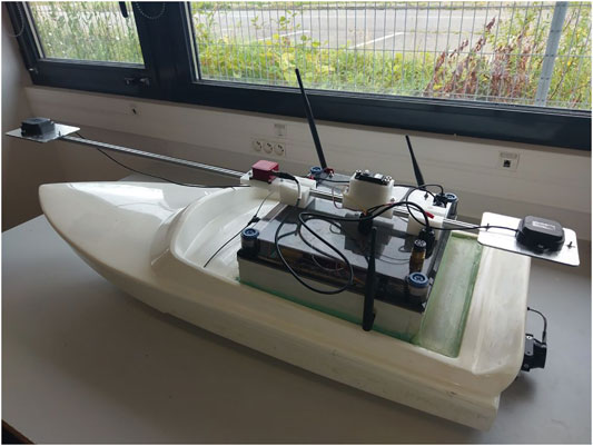
An autonomous boat has been used to demonstrate the use of interval methods for heading and position estimation (see Figure 1).

FIGURE 1

FIGURE 1. Autonomous boat with an interval-based inertial navigation system (INS).

It is based on a 1-m long hull (MHZ PowerBoats Jetsprint-Jetboat) that is equipped with a jet propeller (MHZ PowerBoats Jet 52) to control its speed and with a servomotor to control the direction of the water jet. On the boat we have:

• A dual GPS (ArduSimple simpleRTK2B+heading, with two u-blox GNSS multiband antennas ANN-MB-00) to get the absolute position, speed over ground (SOG), course over ground (COG), as well as true heading of the robot (note although it could be possible, we did not use RTK corrections for the position estimates).

• An AHRS (SBG Ellipse2-A-G4A3-B1, with full scale of gyrometers of 450°/s and accelerometers of 16 g) to get the Euler angles and their derivates. Note that the accelerometers inside are not precise enough to estimate correctly the position; they are only used internally for the angle computations.

• A DVL (Teledyne Wayfinder), to get the forward and lateral speed of the robot, especially when exploring narrow rivers, where GPS obstructions may occur on its banks. The distance to the river floor is also measured and can be used to generate a height map of the covered area.

More information about the design of this autonomous boat is available in Sanchez (2021).

2.5 Interval-Based Inertial Navigation System

2.5.1 Principle of Operation

The purpose of this first interval-based INS is to estimate reliably the heading ψ of the boat as an interval $\left[\psi \right]$, using the dual GPS of the boat, which gives an estimation ψ_GPS, the gyrometers of the AHRS ω (rotation around the vertical axis), and the magnetometers of the AHRS, which gives an estimation ψ_mag (we will assume here that the magnetic declination and any physical bias between the sensors have been already taken into account, or their uncertainties are within the width of the intervals). It is possible to describe our problem as follows:

$\begin{array}{l}\hfill \left\{\begin{array}{cc}\dot{\mathbf{x}}\hfill & =\mathbf{f}\left(\mathbf{x}\right)\left(\mathrm{e}\mathrm{v}\mathrm{o}\mathrm{l}\mathrm{u}\mathrm{t}\mathrm{i}\mathrm{o}\mathrm{n}\mathrm{e}\mathrm{q}\mathrm{u}\mathrm{a}\mathrm{t}\mathrm{i}\mathrm{o}\mathrm{n}\right)\hfill \\ \mathbf{y}\hfill & =\mathbf{g}\left(\mathbf{x}\right)\left(\mathrm{o}\mathrm{b}\mathrm{s}\mathrm{e}\mathrm{r}\mathrm{v}\mathrm{a}\mathrm{t}\mathrm{i}\mathrm{o}\mathrm{n}\mathrm{e}\mathrm{q}\mathrm{u}\mathrm{a}\mathrm{t}\mathrm{i}\mathrm{o}\mathrm{n}\right)\hfill \\ \mathbf{0}\hfill & =\mathbf{h}\left(\mathbf{x}\right)\left(\mathrm{c}\mathrm{o}\mathrm{n}\mathrm{s}\mathrm{i}\mathrm{s}\mathrm{t}\mathrm{e}\mathrm{n}\mathrm{c}\mathrm{y}\mathrm{e}\mathrm{q}\mathrm{u}\mathrm{a}\mathrm{t}\mathrm{i}\mathrm{o}\mathrm{n}\right)\hfill \end{array}\right.\end{array}(1)$

where $\mathbf{x}(t)=\left(\begin{array}{c}\hfill \cos \left(\psi (t)\right)\hfill \\ \hfill \sin \left(\psi (t)\right)\hfill \end{array}\right)$ is the state vector, $\mathbf{y}(t)=\left(\begin{array}{c}\hfill \cos \left({\psi }_{\text{GPS}}(t)\right)\hfill \\ \hfill \sin \left({\psi }_{\text{GPS}}(t)\right)\hfill \\ \hfill \cos \left({\psi }_{\text{mag}}(t)\right)\hfill \\ \hfill \sin \left({\psi }_{\text{mag}}(t)\right)\hfill \end{array}\right)$ is the output vector, $\mathbf{f}(\mathbf{x})=\left(\begin{array}{cc}\hfill 0\hfill & \hfill -\omega \hfill \\ \hfill \omega \hfill & \hfill 0\hfill \end{array}\right)\mathbf{x}$, $\mathbf{g}(\mathbf{x})=\left(\begin{array}{c}\hfill x_1\hfill \\ \hfill x_2\hfill \\ \hfill x_1\hfill \\ \hfill x_2\hfill \end{array}\right)$, and $\mathbf{h}(\mathbf{x})=x_1^2+x_2^2-1$. We will assume that:

• For all $t\in \left[t_0,t_f\right]$, we have intervals enclosing ω(t):

$\forall t\in \left[t_0,t_f\right],\omega \left(t\right)\in \left[\mathit{\omega }\right]\left(t\right);(2)$

• For multiple time instants $t_i\in \left[t_0,t_f\right]$, we have intervals enclosing ψ_GPS(t_i):

$\exists t_i\in \left[t_0,t_f\right],{\psi }_{\text{GPS}}\left(t_i\right)\in \left[{\psi }_{\text{GPS}}\right]\left(t_i\right);(3)$

• For all $t\in \left[t_0,t_f\right]$, we have intervals enclosing ψ_mag(t):

$\forall t\in \left[t_0,t_f\right],{\psi }_{\text{mag}}\left(t\right)\in \left[{\psi }_{\text{mag}}\right]\left(t\right).(4)$

In 2D, the vertical gyrometer is measuring the heading velocity, so we have:

$\dot{\psi }=\omega .(5)$

If we apply at each time step the contraction procedure described in the Data fusion with interval analysis section, the observation equation in combination with Eq. (3) will provide precise intervals for $\left[\psi \right]$ at regular time instants⁵ (from $\left[{\psi }_{\text{GPS}}\right]$ if the GPS is available and the distance between the two antennas is considered consistent with the user-provided antenna distance, or from $\left[{\psi }_{\text{mag}}\right]$ otherwise), while Eqs. (5) and (2) should propagate an estimation for other time intervals. For that, we could discretize the differential Eq. 5 using the Euler method, i.e., $\psi \left(t+dt\right)=\psi \left(t\right)+dt\cdot \omega \left(t\right)$; however, in practice manipulations such as additions and comparisons directly on angles are not recommended due to the modulo 2π (or 360°) equivalence of angles. Instead, we can use the cos and sin of the angles, so if $\mathbf{x}(t)=\left(\begin{array}{c}\hfill \cos \left(\psi (t)\right)\hfill \\ \hfill \sin \left(\psi (t)\right)\hfill \end{array}\right)$, due to Eq. 5, we have $\dot{\mathbf{x}}(t)=\left(\begin{array}{c}\hfill -\omega (t)\sin \left(\psi (t)\right)\hfill \\ \hfill \omega (t)\cos \left(\psi (t)\right)\hfill \end{array}\right)$ (evolution equation). This can be written as $\dot{\mathbf{x}}=\mathbf{A}\mathbf{x}$ with $\mathbf{A}=\left(\begin{array}{cc}\hfill 0\hfill & \hfill -\omega \hfill \\ \hfill \omega \hfill & \hfill 0\hfill \end{array}\right)$, and additionally, it is possible to find an exact solution for this type of differential equation, as $\mathbf{x}\left(t\right)=k\exp \left(\mathbf{A}\cdot t\right)$ if ω is assumed to be a piecewise constant (i.e., A is not varying much during the time step dt). By writing $\mathbf{x}\left(t+dt\right)$ with respect to $\mathbf{x}\left(t\right)$, it can be discretized as $\mathbf{x}\left(t+dt\right)=\exp \left(\mathbf{A}dt\right)\mathbf{x}\left(t\right)$. If A is antisymmetric, $\exp \left(\mathbf{A}dt\right)$ is a rotation matrix, of angle ω ⋅ dt in our case. Although not strictly necessary, it is also possible to use the equation $x_1^2+x_2^2=1$ (consistency equation) to try to limit potential overestimation of the uncertainty when evaluating $\left[\cos \left(\psi (t)\right)\right]$ and $\left[\sin \left(\psi (t)\right)\right]$. Then the polar contractor from Desrochers and Jaulin (2016b) ⁶ can be used to contract $\left[\psi \right]$ from $\left[\cos \left(\psi (t)\right)\right]$ and $\left[\sin \left(\psi (t)\right)\right]$. If an empty set appears at any time during the contraction procedure at a time step, $\left[\psi \right]$ is set to its last known value.

2.5.2 Comparison With Alternative Systems

To get a first validation of the interval-based INS designed, comparisons with other systems have been made⁷. A first experiment has been set up with a high-end iXBlue QUADRANS Fiber-Optic Gyrocompass (FOG) INS (see Figure 2) as a kind of ground truth to get a first idea on the precision of our system. Both systems have been mounted together and moved manually with various rotations and oscillations at different speeds (only planar movements, see Figures 3 and 4). The mean error and the standard deviation between the systems are both around 1.5°, which means that there was probably a physical bias of 1.5° between the two systems, and assuming the QUADRANS is the ground truth (specifications suggest an error of less than 0.2°), the interval-based INS has a typical error of 1.5°⁸, which seems small enough for the autonomous boat used as a target system to be able to follow a track within the typical precision of a standard GPS, as it will be demonstrated in the Online control results in real experiments section (also, note that the typical error of an SBG Ellipse2-A-G4A3-B1, whose hardware—especially the gyrometers—is used in the interval-based INS, is around 1°).

FIGURE 2

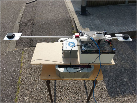
FIGURE 2. The iXBlue QUADRANS INS mounted together with the hardware of the interval-based INS. The QUADRANS was in the opposite direction of the rest and outputting data at 50 Hz, while the interval-based INS was operated at 20 Hz. Note that the QUADRANS did not have GPS, since it is not required for its operation and to be in conditions as different as possible from the rest of the system.

FIGURE 3

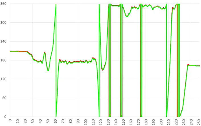
FIGURE 3. Evolution of the heading (in ° with respect to time in s) of the interval-based INS (in red) and the QUADRANS (in green). They visually coincide all the time except briefly sometimes due to the modulo 360° effect and fast movements (fast w.r.t. temporal resolution).

FIGURE 4

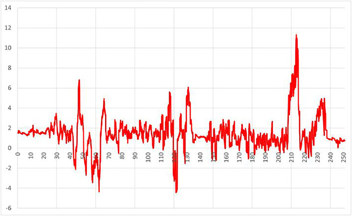
FIGURE 4. Evolution of the heading error (in ° with respect to time in s) between the interval-based INS and the QUADRANS.

The purpose of the second batch of experiments is to demonstrate that the interval-based INS could be competitive compared with existing solutions in some scenarios where faults or inconsistencies between sensors occur. Contrary to the preceding experiment, we are not interested in precision but rather in the behavior when handling obvious outliers. For that, two other systems were tested: an SBG Ellipse3-D-G4A2-B2 (with gyrometers full scale of 450°/s and accelerometers of 8 g) with SDK 6.2 and a Pixhawk 4 mini [firmware ArduRover V4.1.0-dev (12 645 674)] with simpleRTK2B+heading–Basic Starter Kit [firmware UBX_F9_100_HPG_113_ZED_F9P configured with instructions from ArduSimple (2021)]. Both systems are made of three magnetometers, three gyrometers, three accelerometers, and a dual GPS, and they are supposed to provide heading information from a fusion of all these sensors, similar to the interval-based INS of the boat. For all systems, default settings were used with magnetometers disabled (as long as the GPS is available) and dual antenna settings (approximately 1 m between the antennas, to fit the size of the boat). The antenna type is the same (antenna 1 at 46 cm behind the Ellipse-D, antenna 2 at 58.5 cm in front, set to “Rough lever arm” setting in sbgCenter), and initial date and lever arms are configured where applicable.

The test procedure has been the following:

• The INS is first left at a constant angle oriented toward the South (180°) during some time to ensure it is correctly initialized.

• Then it is turned by 90° toward West (270°) and left around for 30 s before returning to the initial position to check if the heading data are correct if the system is not static.

• To generate an inconsistency between the heading computed from the dual GPS antennas and the gyrometers, the IMU part of the system is rapidly moved to try to saturate the gyrometers and left at a constant angle oriented toward the West around 30 s, while the GPS antennas are not moved at all (therefore, they are still pointing toward the South).

• Finally, the IMU is put back in its original position to check how it recovers from the inconsistency. For the interval-based INS, other movements were made after the inconsistency to check that it was still responding correctly.

Figure 5 shows the results of the experiment for the Ellipse-D. The fused heading and the GPS heading coincide (except that the update rate of the GPS is 5 Hz, while the fused heading is determined at a frequency of 50 Hz) until the gyrometers are saturated. At this point, the fused heading outputs a wrong value of 200°, possibly evaluated from the gyrometer data; however, it does not correspond with the heading of the IMU, which should have been 270° or the heading of the GPS, which should have been 180° at this point of the experiment. After the IMU is put back in the same direction of the GPS, the fused heading indicates 100°, instead of 180°. It should be noted, however, that in other tests, where the gyrometer saturation was probably shorter, the Ellipse-D was sometimes able to recover from that disturbance. Also, although not tested, it might be possible to make it trust more the GPS instead of the gyrometers with other settings. Indeed, the commercial purpose of this type of INS is probably to be able to be more robust to GPS outliers due to, e.g., multipaths as well as increasing the heading output rate compared with a dual GPS without IMU aid. However, it should be possible to detect easily the gyrometer saturations and to choose in that case automatically to trust more the GPS data as long as they seem to be correct (e.g., distance between antennas still consistent with what was evaluated previously and with what was specified by the user as the initial value), as it was the case in this experiment.

FIGURE 5

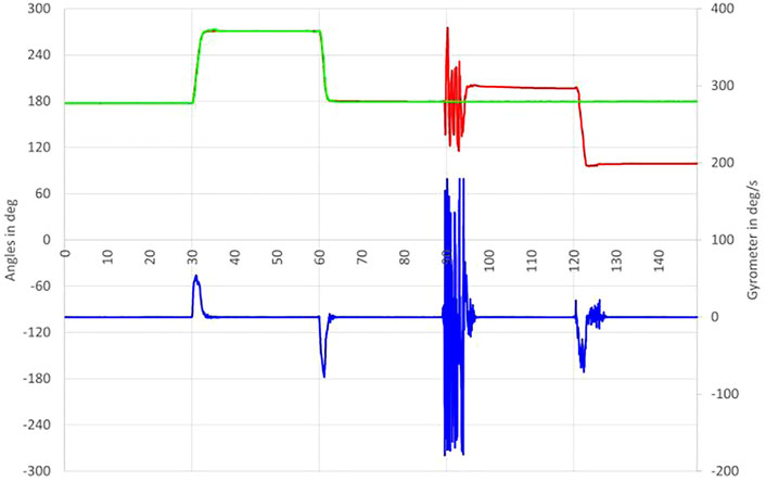
FIGURE 5. Evolution of the heading (in red) for the Ellipse-D (in ° with respect to time in s). The raw heading from the GPS is in green (in °), and the gyrometer data is in blue (in °/s).

Figure 6 shows the results of the experiment for the Pixhawk. The fused heading and the GPS heading coincide (except the update rate of the GPS is 5 Hz, while the fused heading is determined at a frequency of 50 Hz) until the gyrometers are saturated. At this point, the fused heading seems off but converges slowly toward the GPS value, until the IMU is moved back in the same direction of the GPS, when the gyrometers detect the rotation even though the fused heading seems again to converge finally toward the GPS value. This is probably due to a continuous weighted fusion between GPS and gyrometers data, which seems to be consistent with the fact that an EKF (Extended Kalman Filter) is known to be used internally (as this is an open-source design, this could be checked in more detail)⁹.

FIGURE 6

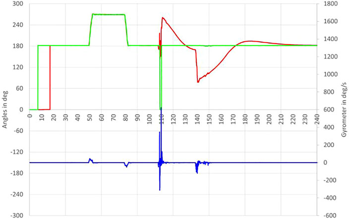
FIGURE 6. Evolution of the heading (in red) for the Pixhawk (in ° with respect to time in s). The raw heading from the GPS is in green (in °), and the gyrometer data is in blue (in °/s).

Figure 7 shows the results of the experiment for the interval-based INS. The fused heading and the GPS heading coincide (except that the update rate of the GPS is 1 Hz, while the fused heading is 20 Hz) except for a short time (1–2 s) when the gyrometers are saturated or when the IMU is moved back to its original position after the saturation. It could be interesting to check in further experiments whether a GPS rate of 5 Hz (like in the Ellipse-D) would give better results especially in the experiment with the QUADRANS, since it is not expected that it would significantly change the behavior in the experiment of Figure 7.

FIGURE 7

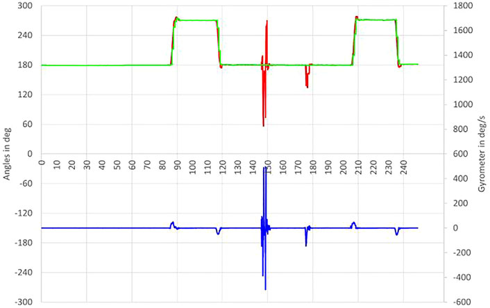
FIGURE 7. Evolution of the heading (in red) for the interval-based INS (in ° with respect to time in s). The raw heading from the GPS is in green (in °) and the gyrometer data is in blue (in °/s).

Although many improvements can already be foreseen, those results show that designing an interval-based INS naturally leads to consider which solution should be returned in case of inconsistencies in the data fusion process (i.e., empty intervals at some point in the computations). This can help to determine better when there are sensors that contradict each other and, whenever possible, which. Even if at the moment, it is not demonstrated that the designed interval-based INS would surpass other existing devices or methods, especially in terms of precision and accuracy, the foreseen theoretically increased reliability (with respect to inconsistencies, with a better propagation of all sensor and model errors, etc.) is alone worth to be reported, and this fact is already experimentally proven by the previously described experiments, which enable us to conclude that it appears to be better than COTS devices at least in some specific situations where inconsistencies could occur¹⁰.

2.6 Jet-Boat Simulator

The boat described in the Description of the autonomous boat section can be simulated using the following model:

$\begin{array}{l}\hfill \left\{\begin{array}{cc}\dot{x}\hfill & =v_x\hfill \\ \dot{y}\hfill & =v_y\hfill \\ \dot{\psi }\hfill & =\frac{\left(v_x\cos \left(\psi \right)+v_y\sin \left(\psi \right)\right)\sin \left(\beta u_2\right)}{L/2}\hfill \\ {\dot{v}}_x\hfill & =\alpha u_1\cos \left(\beta u_2\right)\cos \left(\psi \right)-{\alpha }_f\left(1+\left|\sin \left(\beta u_2\right)\right|\right)v_x\hfill \\ {\dot{v}}_y\hfill & =\alpha u_1\cos \left(\beta u_2\right)\sin \left(\psi \right)-{\alpha }_f\left(1+\left|\sin \left(\beta u_2\right)\right|\right)v_y,\hfill \end{array}\right.\end{array}(6)$

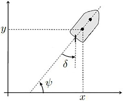
where x and y are the boat coordinates, ψ its heading, v_x and v_y, the corresponding velocities in x and y directions, u₁ is the motor input, and u₂ is the jet direction input (see Figure 8). To significantly simplify the equations, the damping coefficient α_f is assumed to be the same in all the directions with respect to the hull, L is the length of the boat, α is a coefficient such that αu₁ is the propelling force, and β is such that δ = βu₂ is the angle of the jet. The expression $v_{rx}=\left(v_x\cos \left(\psi \right)+v_y\sin \left(\psi \right)\right)$ corresponds to the longitudinal speed of the boat expressed in the boat coordinate system. We assume that the jet direction acts as a rudder since even when u₁ = 0, the water flowing through the jet (which is only due to v_rx and not much the lateral speed $v_{ry}=\left(v_y\cos \left(\psi \right)-v_x\sin \left(\psi \right)\right)$) can still rotate the boat a little. Also, the longitudinal speed decreases when the angle of the jet is not neutral (generating rotation without lateral speed, which is mainly due to inertia), which corresponds to the $\cos \left(\beta u_2\right)$ and $1+\left|\sin \left(\beta u_2\right)\right|$ terms in the expressions of the accelerations. Water current speed components can be easily added to $\dot{x}$ and $\dot{y}$ in the model, which would implicitly define a new coordinate system translating with the current. This model is used to build an interval observer for position estimation in the Results section.

FIGURE 8

FIGURE 8. Description of the variables in the simulated boat model.

Figure 9 presents a simulated boustrophedon track (typical pattern followed by survey vessels, lawnmowers, etc.) with the same waypoints as the real experiment that is described in the Online control results in real experiments section. The coefficients in the model have been manually set so that the simulated track closely fits the real one. The control algorithm used is similar to the simple line following controller described in Jaulin and Le Bars (2012a) (only the rudder control is used in our case, the motor input was constant or manual). Additional tests when manually controlling the inputs show that the behavior of the simulated boat is similar to the real one.

FIGURE 9

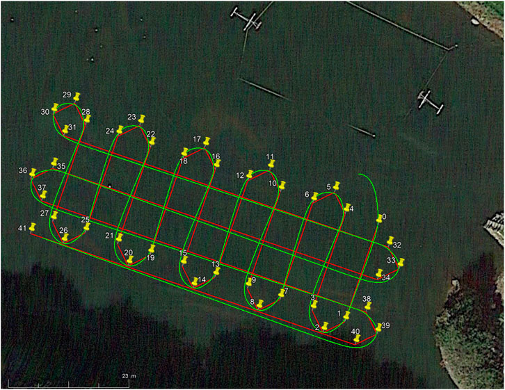
FIGURE 9. The simulated boustrophedon track (in green) with the desired waypoints (in yellow, connected by red lines). Short legs are approximately 20 m and long ones are 70 m.

3 Results

This section discusses the experiments made with the autonomous boat previously described, in different scenarios. All the data and the corresponding processing methods are available at http://www.ensta-bretagne.fr/lebars/spebot/ (see also footnote 7).

3.1 Online Control Results in Real Experiments

To demonstrate that the designed interval-based INS can be used in real missions of outdoor autonomous robots, the boat described in the Description of the autonomous boat section has been programmed to follow the boustrophedon track presented in the Jet-boat simulator section on a river. In the embedded controller, the heading computed by the interval-based INS is used to follow a target heading, which can be defined by the direction to follow to go toward a target waypoint [case of a simple waypoint following controller, see, e.g., Jaulin (2009)], or a weighted combination between this direction and the distance to the line between the previous waypoint and the target waypoint [case of a line following controller, see, e.g., Jaulin and Le Bars (2012a)]. Figure 10 shows that the trajectory is indeed compatible with what could be expected for this type of mission, with a maximum distance of around 2.5 m from the lines between the waypoints. Inaccurate heading estimations would make the robot often miss the target waypoint (and, in worst cases, go back to it and even turn around without managing to reach a desired minimum distance) in case of a waypoint-following controller, or oscillate near the line in case of a line-following controller (assuming the waypoints are reachable taking into account the robot dynamics).

FIGURE 10

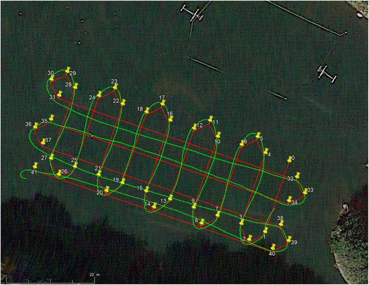
FIGURE 10. The real boustrophedon track (in green) with the desired waypoints (in yellow, connected by red lines). Short legs are approximately 20 m and long ones are 70 m.

3.2 Additional Tests and Offline Processing

3.2.1 Offline Processing to Fuse GPS Data with the Model

Since GPS only provides a new position estimate every second, the boat model used in the Jet-boat simulator section could be used to enhance the state estimation with an improved temporal resolution, e.g., by following the method in Le Bars et al. (2018) (and the problem is somehow similar to the fusion between gyrometer and GPS heading described in the Principle of operation section). In this context, we can describe our problem as:

$\begin{array}{l}\hfill \left\{\begin{array}{cc}\dot{\mathbf{x}}\hfill & =\mathbf{f}\left(\mathbf{x},\mathbf{u}\right)\left(\text{evolution\hspace{0.17em}equation}\right)\hfill \\ \mathbf{y}\hfill & =\mathbf{g}\left(\mathbf{x}\right)\left(\text{observation\hspace{0.17em}equation}\right),\hfill \end{array}\right.\end{array}(7)$

where x(t) is the state vector of the boat, u(t) is its input vector, y(t) is its output vector, and:

• For some time instant t₀, we have a box $\left[\mathbf{x}\right]\left(t_0\right)$ containing the state vector:

$\mathbf{x}\left(t_0\right)\in \left[\mathbf{x}\right]\left(t_0\right);(8)$

• For all $t\in \left[t_0,t_f\right]$, we have boxes enclosing u(t):

$\forall t\in \left[t_0,t_f\right],\mathbf{u}\left(t\right)\in \left[\mathbf{u}\right]\left(t\right);(9)$

• For multiple time instants $t_i\in \left[t_0,t_f\right]$, we have boxes enclosing y (t_i):

$\exists t_i\in \left[t_0,t_f\right],\mathbf{y}\left(t_i\right)\in \left[\mathbf{y}\right]\left(t_i\right).(10)$

The evolution equation is given by Eq. (6), and the observation equation is:

$\mathbf{y}=\left(\begin{array}{c}\hfill x\hfill \\ \hfill y\hfill \\ \hfill \psi \hfill \end{array}\right)(11)$

because (x, y) can be measured regularly (i.e., not at all times) by the GPS, and ψ is measured by the INS at all times.

To solve this problem, we will use the contractor approach described previously:

• First, we need to use the observation equation to contract the known GPS positions of the robot.

• Then a propagation with respect to time on the differential equation [i.e., Eq. (6)] discretized using, for example, the explicit Euler method can be employed to get an evaluation of the trajectory between GPS positions.

• Repeating all the previous contraction operations until no more significant improvement on the trajectory estimation is achievable should propagate the contractions performed at selected points through the whole trajectory.

Remember also that any interval for which we do not have specific initial data first needs to be initialized as wide as possible to stay consistent with any further data, but $\left[-\infty ,\infty \right]$ should only be used as a last resort to minimize the risk that no contraction can occur. In practice, we can almost always assume a bounded position and speed due to the physical limitations of the system in its actual operating conditions.

3.2.2 Dead Reckoning In Case Of GPS Loss Without Speed Sensor

The approach described in the previous section works also if we simulate the loss of the GPS position during a large portion of time (note that although the heading logs are here from the dual GPS, the system would have fell back to magnetometer in case of real GPS loss, which has no specific influence on the problem described in this section). During the loss of the GPS, the uncertainties will quickly increase over time (typical problem of dead reckoning), which translates to intervals (or boxes in 2D) with an increasing width, as explained in Le Bars et al. (2018). Figure 11 illustrates the trajectory estimation of the boat assuming the GPS was lost after 150 s, and details about the estimation of x and y are depicted in Figures 12 and 13 (see the Interval analysis section for more details about tubes). The figures have been generated in a computing time of around 30 s using the Codac library [see Rohou (2021)] and VIBes [see Drevelle and Nicola (2014)]. The GPS accuracy when it is in use is assumed to be 2.5 m, and its data are available every second. Additionally, a water current of $\left(0.025;-0.022\right)$m/s (assumed to be uniform, although it is not always the case especially in a river) has been taken into account in the state equation model, and the coefficients α_f = 1.3, α = 11.5, β = 23, and L = 1 have been estimated manually. Since most of the model uncertainties are likely to be related to the damping, it is assumed that ${\alpha }_f\in 1.3+\left[-0.02;0.02\right]$ to ensure consistency of the model with the real positions. Therefore, the overall envelope of the trajectory estimation stays around a width of 5 m as long as the GPS is in use, but grows over time as soon as no position information is available any more. Despite the large uncertainty even at the last position, it is close to the GPS estimation if the center of the x and y intervals are taken as first approximation (which is often the most likely to be close to reality, similar to what a Kalman filter would do). During the period when the GPS is taken into account, it is assumed that the position it gives is the one at the time of reception of the data, i.e., this approximation is assumed to be within the width of the corresponding interval, which is 5 m. Due to this, it is allowed that the GPS trajectory (which is a step function) exits the position envelope, as long as it is at less than 2.5 m.

FIGURE 11

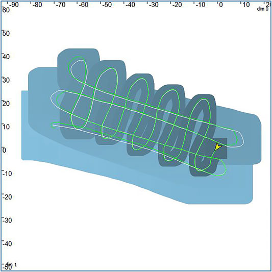
FIGURE 11. The trajectory estimation of the boat assuming the GPS cannot be used after 150 s (scale is in m). The GPS position data (considered as ground truth) are in green and the trajectory is displayed as a blue tube whose center is in white (the beginning corresponds to the darkest box).

FIGURE 12

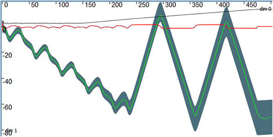
FIGURE 12. The x position (in m) over time (in s) displayed as a tube in gray, GPS x position in green (in m), speed estimation (in m/s) tube in red, and error (in m) as the half-width of the tube (in black).

FIGURE 13

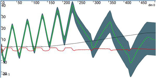
FIGURE 13. The y position (in m) over time (in s) displayed as a tube in gray, GPS y position in green (in m), speed estimation (in m/s) tube in red, and error (in m) as the half-width of the tube (in black).

3.2.3 Dead Reckoning in Case of GPS Loss with a Speed Sensor

As mentioned in the Description of the autonomous boat section, a DVL sensor has been installed on the boat for some experiments. Therefore, a state estimation method inspired from, e.g., Le Bars et al. (2010) can be used (as a comparison, for a Kalman-based method, see, e.g., Reitbauer and Schmied (2021). There, a similar problem is simulated for a ground robot. Odometers in combination with a Kalman filter are used to get the vehicle speed). Indeed, if $\mathbf{p}=\left(\begin{array}{c}\hfill x\hfill \\ \hfill y\hfill \end{array}\right)$ is the position of the robot, v_r is the speed vector measured directly by the DVL, and R is the Euler rotation matrix measured by the INS¹¹, we have:

$\dot{\mathbf{p}}=\mathbf{R}\cdot {\mathbf{v}}_r.(12)$

We can assume that:

• For some time instant t₀, we have a box $\left[\mathbf{p}\right]\left(t_0\right)$ containing the state vector:

$\mathbf{p}\left(t_0\right)\in \left[\mathbf{p}\right]\left(t_0\right);(13)$

• For all $t\in \left[t_0,t_f\right]$, we have boxes enclosing R(t) and v_r(t):

$\forall t\in \left[t_0,t_f\right],\mathbf{R}\left(t\right)\in \left[\mathbf{R}\right]\left(t\right)\mathrm{a}\mathrm{n}\mathrm{d}{\mathbf{v}}_r\left(t\right)\in \left[{\mathbf{v}}_r\right]\left(t\right).(14)$

A propagation with respect to time on the differential Eq. 12 discretized using the explicit Euler method can be used to get an evaluation of the trajectory. Figure 14 illustrates the trajectory estimation of the boat assuming the GPS was lost after 20 s, and details about x and y estimations are visualized in Figures 15 and 16. Contrary to the previous situation without DVL, the position uncertainty grows slower when the GPS is not available anymore. There are also moments where the model is close to be inconsistent with the GPS position in Figure 15, although it is not a problem due to the GPS uncertainties as explained before¹².

FIGURE 14

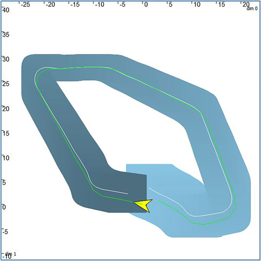
FIGURE 14. The trajectory estimation of the boat assuming the GPS cannot be used after 20 s, with DVL (scale is in m). The GPS position data (considered as ground truth) are in green, and the trajectory is displayed as a blue tube whose center is in white (the beginning corresponds to the darkest box).

FIGURE 15

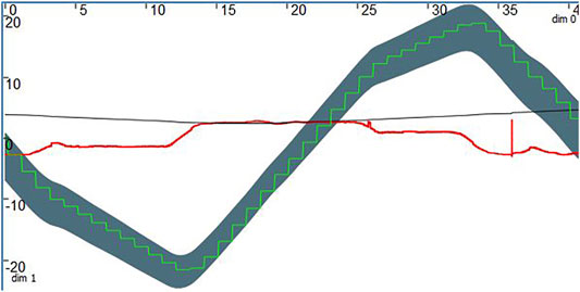
FIGURE 15. The x position (in m) over time (in s) displayed as a tube in gray, GPS x position in green (in m), speed estimation (in m/s) tube in red, and error (in m) as the half-width of the tube (in black).

FIGURE 16

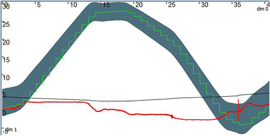
FIGURE 16. The y position (in m) over time (in s) displayed as a tube in gray, GPS y position in green (in m), speed estimation (in m/s) tube in red, and error (in m) as the half-width of the tube (in black).

Whatever the sensors or model used, these results demonstrate that interval methods can naturally provide a reliable estimation of the position error during the survey. The consistency with the GPS position considered as ground truth validates also that the interval-based INS used inside the boat outputs correct data. As long as the different hypotheses are true (e.g., assumptions on the precision of the discretized model, sensors data, etc.), the system can then theoretically provide a guaranteed explored, potentially explored, and surely not explored area as proposed in Desrochers and Jaulin (2016a) (here the position of the boat is in some way considered as the explored area, but in practice, the payload sensor characteristics should be used, and e.g., it would be the explored underwater area that would need to be guaranteed for the search of a target underwater).

Note that there were boat dynamic problems due to the DVL shape, the use of a smaller DVL such as Water Linked (2021), or improving its mechanical integration in the hull could easily limit the disturbances.

4 Conclusions and Outlook on Future Work

The reliable state estimation of an autonomous boat for river exploration has been presented in this paper. The main contribution is a first design of an interval-based INS, where the heading estimation is obtained from the fusion of dual GPS and gyrometer data in combination with a simple differential equation model, using interval analysis. Unit tests show that the precision and accuracy are compatible with the typically expected precision of the hardware, and in addition, some scenarios show a better resilience to outliers compared with alternative systems. The experiments made with an autonomous boat demonstrate the practical applicability of the approach.

Currently, it has to be noted that the described interval-based INS does not use interval analysis yet for roll and pitch, and the yaw used as fallback in case of GPS loss is not from the raw magnetometers from the SBG Ellipse-A underlying hardware, although no specific obstacle is foreseen for those improvements. Additionally, the system is not expected to be much robust to some GPS disturbances such as spoofing: Currently, it should fall back to the magnetometers in case the GPS is lost, or the estimated distance between the antennas is inconsistent, but sending misleading yet valid and consistent GPS data would make the system behave as if it was the other heading-related sensors that are failing, which should be also possible to take into account better in future work. Handling differential equation models $\dot{\mathbf{x}}=\mathbf{f}(\mathbf{x},\mathbf{u})$ in the general case without discretizing using the explicit Euler method to estimate the state, assuming we have an initial condition, is currently also an open issue. Indeed, although the propagation with respect to time in Eq. 12 can be done successfully using the tube differential contractor described in Rohou et al. (2017), it will not be able to efficiently contract the model (6). The Lohner contractor proposed by Bourgois (2021) solves the problem of the generic differential contractor in the case where $\dot{\mathbf{x}}=\mathbf{f}(\mathbf{x})$; however, this still cannot be applied directly to Eq. (6) due to the inputs (which are typically interval quantities without any knowledge about temporal variations within their bounds and could come from a control algorithm and/or the user teleoperating the boat).

Data Availability Statement

The datasets presented in this study can be found in online repositories. The names of the repository/repositories and accession number(s) can be found below: http://www.ensta-bretagne.fr/lebars/spebot/.

Author Contributions

All authors listed have made a substantial, direct, and intellectual contribution to the work and approved it for publication.

Funding

This work was supported by the French Government Defense Procurement and Technology Agency (DGA).

Conflict of Interest

The authors declare that the research was conducted in the absence of any commercial or financial relationships that could be construed as a potential conflict of interest.

Publisher’s Note

All claims expressed in this article are solely those of the authors and do not necessarily represent those of their affiliated organizations, or those of the publisher, the editors, and the reviewers. Any product that may be evaluated in this article, or claim that may be made by its manufacturer, is not guaranteed or endorsed by the publisher.

Footnotes

¹Unmanned Aerial/Surface/Ground/Underwater Vehicle, the letter U is often replaced by the letter A for Autonomous when the vehicle is unmanned and can be autonomous, which will be in the scope of this paper.

²For simplicity, GPS (Global Positioning System) and GNSS (Global Navigation Satellite System) notations will be used equally in the rest of the paper even though multiple constellations might be employed internally by the devices used.

³Basic factorization steps are usually not detailed although they might be necessary at implementation time to achieve a good precision performance.

⁴The implementation of this example in Python is available at http://replit.com/@lebarsfa/IntervalContractionProcedure.

⁵In practice, the time delay between the moment when the GPS heading was received and the moment for which this value has been measured needs to be estimated as precisely as possible, see Sanchez (2021) for more details and also Le Bars et al. (2012), Rohou et al. (2018) and Kletting et al. (2006) in case of time-varying uncertainties.

⁶An implementation of the polar contractor is available in the Codac library (see Rohou (2021)). Since it currently appears to be precise only for $\left[-\pi /2,\pi /2\right]$ (there might be overestimation of the uncertainty for angles around − π), a pre-processing has been made to ensure that the results remain precise in $\left[-\pi ,\pi \right]$ by changing the sign of $\left[x_1\right]$ if $x_1^{+}<0$ before applying the contractor and then negating the result and adding π, see Sanchez (2021) for more details.

⁷All experimental data are available at http://www.ensta-bretagne.fr/lebars/spebot/.

⁸With a potentially non-optimal time synchronization between data, and without specific effort to optimize the accuracy or precision, it has especially been noted during the experiment that the mounting of the antennas was not rigid enough.

⁹For an unknown reason (potentially a temporary bad connection or minor problem in the recording of the data), the heading from the GPS seems to drop punctually when the IMU part is moved rapidly, even though this does not seem to cause specific problems.

¹⁰It has to be noted that since many profiles or parameters are available in the systems used, the behavior might differ if settings other than the defaults were used.

¹¹To simplify, we have assumed that the movement of the robot is only in 2D even though it can be easily extended to 3D. Any lever arms between sensors are assumed within the estimation errors. Note also it could be interesting to estimate the orientation bias between the DVL and the INS during moments where we have the GPS.

¹²It has to be noted that around t = 35 s in Figures 15 and 16, the speed has a punctual unexpected uncertainty. Although this has few consequences on the final results, it would remain to be investigated (it could be due to a nonoptimality of the cos or sin interval functions (which appear in R ⋅v_r) in the underlying implementation since it seems to correspond to an angle of π).

References

[Dataset] ArduPilot (2021a). ArduPilot. Available at: http://www.ardupilot.org/.

Google Scholar

[Dataset] ArduPilot (2021b). GPS for Yaw (Aka Moving Baseline). Available at: https://ardupilot.org/copter/docs/common-gps-for-yaw.html.

Google Scholar

[Dataset] ArduSimple (2021). ZED-F9P Firmware Update with simpleRTK2B + Fw Version Check. Available at: https://www.ardusimple.com/zed-f9p-firmware-update-with-simplertk2b/.

Google Scholar

Bonargent, T., Ménard, T., Pigeon, E., Pouliquen, M., and Gehan, O. (2020). “Observer Design for Nonlinear Systems with Multi-Rate Sampled Outputs - Application to Attitude Estimation,” in 2020 European Control Conference (ECC), Saint Petersburg, Russia, May 12–15, 2020, 997–1002. doi:10.23919/ECC51009.2020.9143923

CrossRef Full Text | Google Scholar

Bourgois, A. (2021). “Safe & Collaborative Autonomous Underwater Docking: Interval Methods for Proving the Feasibility of an Underwater Docking Problem. PhD dissertation. France: Université de Bretagne Occidentale, ENSTA Bretagne.

Google Scholar

[Dataset] Chabert, G. (2021). IBEX. Available at: http://www.ibex-lib.org/.

Google Scholar

Chabert, G., and Jaulin, L. (2009). Contractor Programming. Artif. Intelligence 173, 1079–1100. doi:10.1016/j.artint.2009.03.002

CrossRef Full Text | Google Scholar

Desrochers, B., and Jaulin, L. (2016b). A Minimal Contractor for the Polar Equation; Application to Robot Localization. Eng. Appl. Artif. Intelligence 55, 83–92. doi:10.1016/j.engappai.2016.06.005

CrossRef Full Text | Google Scholar

Desrochers, B., and Jaulin, L. (2016a). Computing a Guaranteed Approximation of the Zone Explored by a Robot. IEEE Transaction on Automatic Control 62, 425–430. doi:10.1109/TAC.2016.2530719

CrossRef Full Text | Google Scholar

Desrochers, B., Lacroix, S., and Jaulin, L. (2015). “Set-membership Approach to the Kidnapped Robot Problem,” in 2015 IEEE/RSJ International Conference on Intelligent Robots and Systems (IROS), Hamburg, Germany, September 28–October 02, 2015. doi:10.1109/iros.2015.7353897

CrossRef Full Text | Google Scholar

[Dataset] Desrochers, B. (2021). pyIbex. Available at: https://pypi.org/project/pyibex/.

Google Scholar

Drevelle, V., and Bonnifait, P. (2013). Reliable Positioning Domain Computation for Urban Navigation. IEEE Intell. Transport. Syst. Mag. 5, 21–29. doi:10.1109/mits.2013.2252058

CrossRef Full Text | Google Scholar

Drevelle, V., and Nicola, J. (2014). VIBes: A Visualizer for Intervals and Boxes. Math.Comput.Sci. 8, 563–572. doi:10.1007/s11786-014-0202-0

CrossRef Full Text | Google Scholar

[Dataset] Dronecode (2021). Dronecode. Available at: http://www.dronecode.org/.

Google Scholar

Fischler, M. A., and Bolles, R. C. (1981). Random Sample Consensus. Commun. ACM 24, 381–395. doi:10.1145/358669.358692

CrossRef Full Text | Google Scholar

Ifqir, S., Rauh, A., Kersten, J., Ichalal, D., Ait-Oufroukh, N., and Mammar, S. (2019). “Interval Observer-Based Controller Design for Systems with State Constraints: Application to Solid Oxide Fuel Cells Stacks,” in 2019 24th International Conference on Methods and Models in Automation and Robotics (MMAR), August 26–29, 2019, Miedzyzdroje, Poland, 372–377. doi:10.1109/MMAR.2019.8864718

CrossRef Full Text | Google Scholar

[Dataset] iXBlue (2021). iXBlue. Available at: http://www.ixblue.com/.

Google Scholar

Jaulin, L., Kieffer, M., Didrit, O., and Walter, E. (2001). Applied Interval Analysis, with Examples in Parameter and State Estimation, Robust Control and Robotics. London: Springer-Verlag.

Google Scholar

Jaulin, L., and Le Bars, F. (2012a). “A Simple Controller for Line Following of Sailboats,” in 5th International Robotic Sailing Conference, Cardiff, United Kingdom, September 17–21, 2012 (Cardiff, UK: Springer), 107–119.

Google Scholar

Jaulin, L., and Le Bars, F. (2012b). An Interval Approach for Stability Analysis; Application to Sailboat Robotics. IEEE Transaction on Robotics 29, 282–287. doi:10.1109/TRO.2012.2217794

CrossRef Full Text | Google Scholar

Jaulin, L. (2015). Mobile Robotics. Available at: http://www.iste.co.uk/book.php?id=1538. 1st edition.

Google Scholar

Jaulin, L. (2009). Robust Set-Membership State Estimation; Application to Underwater Robotics. Automatica 45, 202–206. doi:10.1016/j.automatica.2008.06.013

CrossRef Full Text | Google Scholar

Kalman, R. E. (1960). A New Approach to Linear Filtering and Prediction Problems. Trans. AMSE, D, J. Basic Eng. 82, 35–45. doi:10.1115/1.3662552

CrossRef Full Text | Google Scholar

Kletting, M., Rauh, A., Aschemann, H., and Hofer, E. (2006). “Interval Observer Design for Nonlinear Systems with Uncertain Time-Varying Parameters,” in 12th IEEE Intl. Conference on Methods and Models in Automation and Robotics MMAR 2006, Miedzyzdroje, Poland, August 28–31, 2006.

Google Scholar

Le Bars, F., Antonio, E., Cervantes, J., De La Cruz, C., and Jaulin, L. (2018). “Estimating the Trajectory of Low-Cost Autonomous Robots Using Interval Analysis: Application to the euRathlon Competition,” in Marine Robotics and Applications. Editor L. Jaulin (Cham: Springer), 51–68. doi:10.1007/978-3-319-70724-2_4

CrossRef Full Text | Google Scholar

Le Bars, F., Bertholom, A., Sliwka, J., and Jaulin, L. (2010). “Interval SLAM for Underwater Robots; a New experiment,” in NOLCOS 2010, Bologna, Italy, September 01–03, 2010. doi:10.3182/20100901-3-it-2016.00083

CrossRef Full Text | Google Scholar

Le Bars, F., Sliwka, J., Jaulin, L., and Reynet, O. (2012). Set-Membership State Estimation with Fleeting Data. Automatica 48, 381–387. doi:10.1016/j.automatica.2011.11.004

CrossRef Full Text | Google Scholar

Mahalanobis, P. C. (1936). On the Generalised Distance in Statistics. Proceedings of the National Institute of Sciences of India, 49–55. Available at: https://link.springer.com/article/10.1007/s13171-019-00164-5#citeas.

Google Scholar

Mahony, R., Hamel, T., and Pflimlin, J.-M. (2008). Nonlinear Complementary Filters on the Special Orthogonal Group. IEEE Trans. Automat. Contr. 53, 1203–1218. doi:10.1109/TAC.2008.923738.16

CrossRef Full Text | Google Scholar

Meier, L., Tanskanen, P., Fraundorfer, F., and Pollefeys, M. (2011). “PIXHAWK: A System for Autonomous Flight Using Onboard Computer Vision,” in 2011 IEEE International Conference on Robotics and Automation, Shanghai, China, May 9–13, 2011, 2992–2997. doi:10.1109/ICRA.2011.5980229

CrossRef Full Text | Google Scholar

Moore, R. E. (1979). Methods and Applications of Interval Analysis. Philadelphia, PA: SIAM.

Google Scholar

Mourad-Chehade, F., Snoussi, H., Kieffer, M., and Richard, C. (2012). Robust Bounded-Error Tracking in Wireless Sensor Networks. SYSID 2012 (Bruxelles, Belgium) 45, 1097–1102. doi:10.3182/20120711-3-be-2027.00333

CrossRef Full Text | Google Scholar

[Dataset] Paparazzi UAV (2021). Paparazzi UAV. Available at: http://wiki.paparazziuav.org/.

Google Scholar

Paturel, Y., Lacambre, J.-B., Patin, F., and Moynagh, C. (2015). “Inertial Navigation at High Latitude: Trials and Test Results,” in OCEANS 2015 - MTS/IEEE Washington, October 19–22, 2015, Washington D.C, 1–5. doi:10.23919/OCEANS.2015.7401904

CrossRef Full Text | Google Scholar

Premerlani, W., and Bizard, P. (2009). Direction Cosine Matrix IMU: Theory. USA: DIY DRONE.

Google Scholar

Promotion 2021, Robotique autonome (2021). Calibrating a Magnetometer Sensor Using Multiple Methods. Tech. rep., ENSTA Bretagne.

Google Scholar

Rauh, A., and Auer, E. (2010). “Interval Approaches to Reliable Control of Dynamical Systems,” in Computer-assisted Proofs - Tools, Methods and Applications Dagstuhl Seminar Proceedings. Editors B. M. Brown, E. Kaltofen, S. Oishi, and S. M. Rump (Dagstuhl, Germany: Schloss Dagstuhl - Leibniz-Zentrum fuer Informatik, Germany), 09471.

Google Scholar

Reitbauer, E., and Schmied, C. (2021). Bridging GNSS Outages with IMU and Odometry: A Case Study for Agricultural Vehicles. Sensors 21, 4467. doi:10.3390/s21134467

PubMed Abstract | CrossRef Full Text | Google Scholar

Revol, N. (2001). Introduction à l’arithmétique par intervalles. Rapport de recherche 4297.

Google Scholar

Reynet, O., Jaulin, L., and Chabert, G. (2009). “Robust TDOA Passive Location Using Interval Analysis and Contractor Programming,” in Radar 2009, Bordeaux, France, October 12–16, 2009.

Google Scholar

[Dataset] Rohou, S. (2021). Codac. Available at: http://codac.io/.

Google Scholar

Rohou, S., Jaulin, L., Mihaylova, L., Le Bars, F., and Veres, S. M. (2017). Guaranteed Computation of Robot Trajectories. Robotics Autonomous Syst. 93, 76–84. doi:10.1016/j.robot.2017.03.020

CrossRef Full Text | Google Scholar

Rohou, S., Jaulin, L., Mihaylova, L., Le Bars, F., and Veres, S. M. (2018). Reliable Non-Linear State Estimation Involving Time Uncertainties. Automatica 93, 379–388. doi:10.1016/j.automatica.2018.03.074

CrossRef Full Text | Google Scholar

Rohou, S., Jaulin, L., Mihaylova, L., Le Bars, F., and Veres, S. (2019). Reliable Robot Localization. ISTE Group. Available at: http://www.iste.co.uk/book.php?id=1553.

Google Scholar

Sanchez, R. (2021). Fabrication et automatisation d’un drone de surface. Tech. rep., ENSTA Bretagne.

Google Scholar

[Dataset] SBG Systems (2021). SBG Systems. Available at: http://www.sbg-systems.com/.

Google Scholar

Voges, R., and Wagner, B. (2018). “Timestamp Offset Calibration for an Imu-Camera System under Interval Uncertainty,” in 2018 IEEE/RSJ International Conference on Intelligent Robots and Systems (IROS), Madrid, Spain, October 1–5, 2018, 377–384. doi:10.1109/IROS.2018.8594237

CrossRef Full Text | Google Scholar

[Dataset] Water Linked (2021). DVL A50. Available at: https://waterlinked.com/product/dvl-a50/.

Google Scholar

Xiong, J., Jauberthie, C., Travé-Massuyès, L., and Le Gall, F. (2013). “Fault Detection Using Interval Kalman Filtering Enhanced by Constraint Propagation,” in 52nd IEEE Conference on Decision and Control, Florence, Italy, December 10–13, 2013, 490–495. doi:10.1109/CDC.2013.675992910.1109/cdc.2013.6759929

CrossRef Full Text | Google Scholar