Linear Parameter Varying Path Tracking Control for Over-Actuated Electric Vehicles

This paper discusses a multi-layer linear parameter varying path tracking controller for autonomous full electric vehicles with 4 wheel drive. Many approaches for path tracking are present in the literature, but the majority of them utilize only the steering wheel. Nowadays, the massive introduction of electric vehicles opens new opportunities for vehicle dynamics control; multiple electric motors, via differential torque, offer an alternative way to influence vehicle motion. The multi-layer structure, managing separately steering wheel and electric motors, permits the exploitation of pre-existing control systems and maintains a straightforward tuning process. Furthermore, the robustness of the path tracking controller is enhanced by introducing tire nonlinearities. Linear parameter varying models offer a direct way to incorporate tire characteristics in the design process. Exploiting ${\mathcal{H}}_{\infty }$ technique the scheduled controller can be seamlessly synthezised. The proposed strategy has been compared in simulation to a benchmark integrated, i.e., a unique controller that manages all the actuators, approach. During double lane changes beyond the vehicle limits, the multi-layer controller guarantees stability and excellent tracking with an average error of 12 and 24 cm on high and low grip respectively.

1 Introduction

Two major trends are driving the automotive industry nowadays. On one hand, self-driving cars promise to reduce road congestion (Stogios et al., 2019), increase safety (Fagnant and Kockelman, 2015) and reduce pollution (Huang et al., 2018). The literature on the topic is very rich. Autonomous driving systems are usually developed around three interacting but separate tasks: sensing and perception, planning, and control (Amer et al., 2017). This paper focuses on the last one: our goal is to track a known, obstacle-free, reference trajectory. Furthermore, trajectory tracking comprises two objectives: to follow a desired path and a reference speed. We circumscribe our work to lateral control: a separate longitudinal controller will track the target velocity. On the other hand, electric vehicles are being massively introduced in the market due to their ecological potentialities (Zinnari et al., 2020; Frieske et al., 2013). Besides environmental aspects, electric vehicles have many advantages; in the context of this work, we are mainly interested in the versatility they offer in terms of drivetrain design. Among the possible drivetrain configurations, the one with 4 electric motors (4WD), one per wheel, offers interesting opportunities for vehicle dynamics control. For example, the possibility to generate a differential torque between left and right wheels permits to influence the vehicle lateral dynamics: this is called torque vectoring (TV). Mainly, TV systems regulate the vehicle yaw rate to improve safety and drivability (Lucchini et al., 2020).

In our work, we consider an autonomous electric vehicle with 4WD. Within this framework, two possibilities exist to control the lateral dynamics: integrated approaches, i.e. techniques that coordinately actuate the steering angle and the motors; or multi-layer approaches, i.e., two controllers that manage respectively the steering angle and the motors.

Integrated approaches are widely discussed in the literature (Goodarzi et al., 2008; Yakub and Mori, 2015; Falcone et al., 2008; Peng et al., 2020). Regarding multi-layer strategies, the single control problems have been investigated in depth. Concerning path tracking, the literature presents many interesting approaches ranging from: Model Predictive Control (MPC) (Guo et al., 2020; Katriniok et al., 2013; Beal and Gerdes, 2013; Falcone et al., 2007; Liniger et al., 2017), sliding mode (Tagne et al., 2013), nonlinear control (Peters et al., 2011), to potential fields (Rossetter et al., 2004). MPC is considered the state of the art. Nevertheless, its use is sensitive to model accuracy and requires a high computational demand. Therefore, MPC implementation entails a non-negligible amount of effort. For TV literature analysis the reader can refer to De Novellis et al., 2014); Kaiser et al., 2014).

However, the interaction of the two control systems is hardly discussed in the literature. Only Chatzikomis et al. (2018) investigate the topic: integrated approaches are compared to a blind (each subsystem is tuned independently) multi-layer structure. The authors highlight the fact that integrated approaches are not robust to friction variation. From a pure control performance standpoint, an integrated approach should be better. However, automotive systems are often built on pre-existing structures and control layers, often designed by different teams, if not different suppliers. Redesigning the entire vehicle dynamics control from scratch would be expensive and discard years of experience and certification efforts. For these reasons, it is interesting and could be beneficial to study the effect of multi-layer approaches.

In this context, the paper designs a nested control structure. The inner control loop uses the electric motors to regulate the yaw rate dynamics. The outer control loop takes care of controlling the steering angle to track a desired trajectory. The core of the scheme is a quasi-linear parameter varying (q-LPV) ${\mathcal{H}}_{\infty }$ controller. It incorporates in an easy way the tire nonlinearities and guarantees a straightforward tuning process. The multi-layer q-LPV/${\mathcal{H}}_{\infty }$, compared to fixed structure and integrated approaches, showed excellent performance. The proposed solutions are validated in simulation with IPG CarMaker on ISO double lane change (DLC) at different velocities and road conditions. This work extends our previous papers (Roselli et al., 2017; Corno et al., 2021) from several standpoints.

1. Differently from the cited literature, we consider an over-actuated vehicle. The control system thus also solves a control allocation problem.

2. The role of the preview distance is better formalized than in Corno. In fact, in Section 3, we introduce the course rate preview control that, to the best of our knowledge, has not been discussed before.

3. We propose a formal way of considering a hierarchical structure by designing a multi-layer controller that explicitly considers the torque vectoring system,

4. We improve the robustness of the path tracking controller by using the q-LPV control structure to consider the tire nonlinearities.

Linear parameter varying (LPV) systems (Mohammadpour and Scherer, 2012) have been extensively used in automotive applications (Li et al., 2021). They have been employed to consider the velocity dependency of the vehicle dynamics (Corno et al., 2021), to schedule a path following controller based on vehicle states (Alcalá et al., 2017), to manage the priority between different actuators (Fergani et al., 2016), or, as in our case, to consider tire nonlinearities (Németh et al., 2016). In particular, since the scheduling parameters are functions of the model state, the system is classified as q-LPV.

To sum up, the contributions of this work are:

• the design of the multi-layer course rate preview structure tuned exploiting the LPV formulation. Especially, the novelty consists in considering the TV system in the designing of the higher level controller;

• a comparison between integrated and multi-layer approaches, highlighting the effectiveness of the proposed approach.

The paper is organized as follows. In Section 2, the models used for control design are presented. Section 3 describes the control structures: a multi-layer ${\mathcal{H}}_{\infty }$ is a necessary step to attain the q-LPV controller. Furthermore, some insight on the parameter choice are given. Section 4 validates the proposed strategies and compares their peculiarities. Finally, Section 5 summarizes the concluding remarks.

2 Vehicle Dynamics Modeling

We describe the vehicle lateral dynamics with the classical single-track model (Abe, 2015):

$\left\{\begin{array}{c}m{a}_y=F_{yf}\cos \left({\delta }_w\right)+F_{yr}\hfill \\ I_z\dot{r}=-F_{yf}{l}_f+F_{yr}{l}_r+M_z\hfill \end{array}\right.(1)$

where a_y is the lateral acceleration, F_{y f,r} are respectively the front and rear lateral tire forces, r is the yaw rate, m the vehicle mass, I_z is the vehicle moment of inertia, l_f,r are the distances from the centre of gravity (CoG) respectively to the front and rear axle, M_z is an external yaw moment, and δ_w is the steering angle at the wheel.

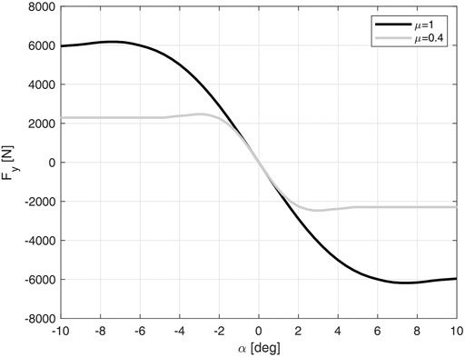
The tire forces are influenced by many parameters and variables, e.g. vertical load F_z, camber angle γ, lateral slip α, longitudinal slip λ, and friction μ. In general:

$F_y=f\left(F_z,\alpha ,\lambda ,\gamma ,\mu \right).(2)$

There exist different ways to describe the nonlinear function f(⋅), e.g., Pacejka (2005); Kiencke and Nielsen (2000); Fiala (1954). Among them, we have preferred the Pacejka’s magic formula for its accuracy. Figure 1 shows an example of f(⋅) for different road surfaces. In this phase, the longitudinal slip is set to 0, and, for the sake of simplicity, also the camber angle is neglected. For a fixed F_z, (Eq. 2) can be linearized around a given lateral slip angle $\bar{\alpha }$:

${\left.F_y\left(\alpha \right)\right|}_{\alpha =\bar{\alpha }}=f\left(\bar{\alpha }\right)+C\left(\bar{\alpha }\right)\left(\alpha -\bar{\alpha }\right)(3)$

where C represents the generalized¹ cornering stiffness defined as:

${\left.C\left(\bar{\alpha }\right)=\frac{\partial f}{\partial \alpha }\right|}_{\alpha =\bar{\alpha }}(4)$

for the sake of clarity, subscripts _f,r for α, F_y, C have been dropped out in the previous relations. To obtain the linear single-track model, we can write the lateral acceleration as:

$a_y=v\left(\dot{\beta }+r\right)(5)$

where v is the vehicle velocity and β is the sideslip angle, i.e., the angle between the single-track longitudinal axis and the velocity vector. Furthermore, with the hypothesis of small angles, we can express the wheel side slips as (Kiencke and Nielsen, 2000):

$\begin{array}{cc}\hfill & {\alpha }_f=\beta +l_f\frac{r}{v}-{\delta }_w\hfill \\ \hfill & {\alpha }_r=\beta -l_r\frac{r}{v}.\hfill \end{array}(6)$

FIGURE 1

FIGURE 1. Tire lateral forces for different friction coefficients at F_z = 6000 N.

Substituting (Eq. 3) (linearized around $\bar{\alpha }=0$), (Eq. 5), and (Eq. 6) in (Eq. 1), the linear single-track model arises:

$\left[\begin{array}{c}\hfill \dot{\beta }\hfill \\ \hfill \dot{r}\hfill \end{array}\right]=\left[\begin{array}{cc}\hfill -\frac{C_f+C_r}{mv}\hfill & \hfill -1+\frac{C_r{l}_r-C_f{l}_f}{m{v}^2}\hfill \\ \hfill \frac{C_r{l}_r-C_f{l}_f}{I_z}\hfill & \hfill -\frac{C_f{l}_f^2+C_r{l}_r^2}{I_{z}v}\hfill \end{array}\right]\left[\begin{array}{c}\hfill \beta \hfill \\ \hfill r\hfill \end{array}\right]+\left[\begin{array}{cc}\hfill \frac{C_f}{mv}\hfill & \hfill 0\hfill \\ \hfill \frac{C_f{l}_f}{I_z}\hfill & \hfill \frac{1}{I_z}\hfill \end{array}\right]\left[\begin{array}{c}\hfill {\delta }_w\hfill \\ \hfill Mz\hfill \end{array}\right](7)$

where C_f = C_f(0) and C_r = C_r(0).

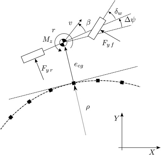
In order to control the vehicle position, the previous model is augmented with its relative motion with respect to a known trajectory (Kapania and Gerdes, 2015). Figure 2 summarizes the main variables. In particular, the dynamics of the heading difference Δψ, i.e., the angle between the vehicle and the trajectory orientation, is

$\dot{\mathrm{\Delta }\psi }=r-\rho v(8)$

where ρ is the trajectory curvature. The lateral error dynamics become:

${\dot{e}}_{cg}=v\left(\beta +\mathrm{\Delta }\psi \right).(9)$

FIGURE 2

FIGURE 2. Augmented single-track variables.

Eventually, we obtain the augmented single-track state space model:

$\left[\begin{array}{c}\hfill \dot{\beta }\hfill \\ \hfill \dot{r}\hfill \\ \hfill \dot{\mathrm{\Delta }\psi }\hfill \\ \hfill {\dot{e}}_{cg}\hfill \end{array}\right]=\left[\begin{array}{cccc}\hfill -\frac{C_f+C_r}{mv}\hfill & \hfill -1+\frac{C_r{l}_r-C_f{l}_f}{m{v}^2}\hfill & \hfill 0\hfill & \hfill 0\hfill \\ \hfill \frac{C_r{l}_r-C_f{l}_f}{I_z}\hfill & \hfill -\frac{C_f{l}_f^2+C_r{l}_r^2}{I_{z}v}\hfill & \hfill 0\hfill & \hfill 0\hfill \\ \hfill 0\hfill & \hfill 1\hfill & \hfill 0\hfill & \hfill 0\hfill \\ \hfill v\hfill & \hfill 0\hfill & \hfill v\hfill & \hfill 0\hfill \end{array}\right]\left[\begin{array}{c}\hfill \beta \hfill \\ \hfill r\hfill \\ \hfill \mathrm{\Delta }\psi \hfill \\ \hfill e_{cg}\hfill \end{array}\right]+\left[\begin{array}{ccc}\hfill \frac{C_f}{mv}\hfill & \hfill 0\hfill & \hfill 0\hfill \\ \hfill \frac{C_f{l}_f}{I_z}\hfill & \hfill \frac{1}{I_z}\hfill & \hfill 0\hfill \\ \hfill 0\hfill & \hfill 0\hfill & \hfill -v\hfill \\ \hfill 0\hfill & \hfill 0\hfill & \hfill 0\hfill \end{array}\right]\left[\begin{array}{c}\hfill {\delta }_w\hfill \\ \hfill M_z\hfill \\ \hfill \rho \hfill \end{array}\right](10)$

where the vector ${\left[\begin{array}{ccc}\hfill {\delta }_w\hfill & \hfill M_z\hfill & \hfill \rho \hfill \end{array}\right]}^{\prime }$ represents the model inputs. δ_w and M_z are control variables; whereas ρ is a measurable disturbance (usually in autonomous driving the path is known in advance).

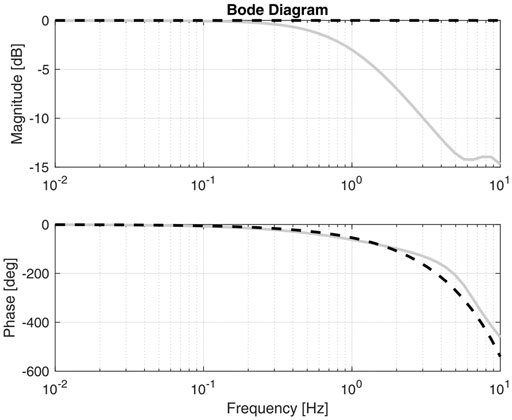
The vehicle model is completed by the actuators dynamics. We consider a fully electric vehicle with 4WD and a steer-by-wire system. Each wheel is connected to an electric motor able to generate both positive and negative torques. Figure 3 plots the static characteristics of the electric motors. A first-order low-pass filter with a bandwidth of 20 Hz and a time delay of 10 ms complete the motor dynamics model.

FIGURE 3

FIGURE 3. Front and rear motors characteristics.

Besides, the steering actuator we consider is composed of an electric motor linked to the steering column via a belt transmission. The system is modeled with a second-order transfer function

$G_{steer}\left(s\right)=\frac{{\omega }_{steer}}{s^2+2{\xi }_{steer}{\omega }_{steer}+{\omega }_{steer}^2}{e}^{-T_{act}s}(11)$

where ω_steer = 2π4.1, ξ_steer = 0.1 and T_act = 0.08 have been experimentally identified (Roselli et al., 2017; Corno et al., 2021).

3 Course Rate Preview Control

In order to control the lateral error, we propose a nested loop approach. The inner loop tracks a desired course rate; it actuates both the steering angle and the motors torque and exploits a preview term usually available in autonomous driving applications. The outer loop corrects the desired course rate based on the actual path tracking error.

We have chosen a multi-layer structure to manage the over-actuated configuration. The course rate controller sets the steering angle; in addition, a standard Torque Vectoring (TV) system generates the motor torques. The scheme in Figure 4 shows the general control structure.

FIGURE 4

FIGURE 4. Multi-layer course rate preview control scheme. The resulting steering wheel command is fed both to the vehicle and to a TV system that generates a suitable yaw moment.

Firstly, for the sake of clarity, we briefly describe the TV block. Afterwards, the course rate preview is designed. Initially, we have adopted the ${\mathcal{H}}_{\infty }$ technique to tune the inner loop. Then, exploiting the same structure, we have applied the ${\mathcal{H}}_{\infty }$ on a LPV version of the single-track in which the tire nonlinearities have been introduced.

3.1 Torque Vectoring

A TV system is generally composed of three blocks (De Novellis et al., 2014): a reference generator, a high-level controller; and a torque allocator.

The reference generator has the objective of providing a suitable yaw rate reference (r_ref). It is defined as in Rajamani (2011):

$r_{ref}=\left\{\begin{array}{cc}\frac{v}{L+v^2{K}_{usdes}}{\delta }_w,\hfill & \text{if\hspace{0.17em}}\left|\frac{v}{L+v^2{K}_{usdes}}{\delta }_w\right|<\frac{0.85\mu g}{v}\hfill \\ \frac{0.85\mu g}{v}\mathrm{sign}\left({\delta }_w\right),\hfill & \text{if\hspace{0.17em}}\left|\frac{v}{L+v^2{K}_{usdes}}{\delta }_w\right|\ge \frac{0.85\mu g}{v}\hfill \end{array}\right.(12)$

where L is the wheelbase, g is the gravitation acceleration, K_{us des} is the desired understeering coefficient. By changing K_{us des} we can impose the desired steering behavior; in our case study, we require a neutral steering vehicle, thus K_{us des} is set to 0.

The high-level controller tracks the desired yaw rate reference by generating a yaw moment. We design this controller using model-based techniques on the nominal transfer function from the yaw moment to the yaw rate obtained from (Eq. 7) at 90 km/h. A PI controller achieves a bandwidth of 1.5 Hz with a phase margin of 80°.

The torque allocator solves the control allocation problem. It distributes the driver torque request to obtain the desired yaw moment. To formulate the optimization problem, we can write a torque balance at vehicle CoG:

$\begin{array}{cc}\hfill M_{ztot}=& \cos \left({\delta }_w\right)\left(F_{xfr}-F_{xfl}\right)\frac{d_f}{2}+\sin \left({\delta }_w\right)\left(F_{xfr}+F_{xfl}\right)l_f+\hfill \\ \hfill & \cos \left({\delta }_w\right)\left(F_{yfr}+F_{yfl}\right)l_f+\sin \left({\delta }_w\right)\left(F_{yfl}-F_{yfr}\right)\frac{d_f}{2}+\hfill \\ \hfill & \left(F_{xrr}-F_{xrl}\right)\frac{d_r}{2}-\left(F_{yrl}+F_{yrr}\right)l_r\hfill \end{array}(13)$

where d_f,r are respectively the front and rear track widths, and F_{x f,r} are the longitudinal tire forces. With the hypothesis of small δ_w (Eq. 13) becomes:

$\begin{array}{cc}\hfill M_{ztot}=& \left(F_{xfr}-F_{xfl}\right)\frac{d_f}{2}+\left(F_{yfr}+F_{yfl}\right)l_f+\hfill \\ \hfill & \left(F_{xrr}-F_{xrl}\right)\frac{d_r}{2}-\left(F_{yrl}+F_{yrr}\right)l_r.\hfill \end{array}(14)$

To influence the lateral dynamics we can exploit the longitudinal forces that are directly controllable with the electric motors. Thus, the yaw moment that can be generated is:

$M_z=\left(F_{xfr}-F_{xfl}\right)\frac{d_f}{2}+\left(F_{xrr}-F_{xrl}\right)\frac{d_r}{2}(15)$

Supposing that a linear relation exists between torque and force: $T_w=\frac{F_x}{R_w}$, where T_w is the torque generated by each electric motor at wheel side, and R_w is the wheel radius; (Eq. 15) can be written as

$u=A\cdot T_v(16)$

where $A=\left[\begin{array}{cccc}\hfill -\frac{d_f}{2R_w}\hfill & \hfill \frac{d_f}{2R_w}\hfill & \hfill -\frac{d_r}{2R_w}\hfill & \hfill \frac{d_r}{2R_w}\hfill \end{array}\right]$ and $T_v={\left[\begin{array}{cccc}\hfill T_{fl}\hfill & \hfill T_{fr}\hfill & \hfill T_{rl}\hfill & \hfill T_{rr}\hfill \end{array}\right]}^{\prime }$. Note that possible inaccuracies introduced by the hypothesis done are compensated by the closed loop control system.

To compute the optimum torque allocation a minimization problem is set:

$\begin{array}{cccc}\hfill & \underset{T_i}{\text{minimize}}\hfill & \hfill & J\left(T_i\right)\hfill \\ \hfill & \text{subject\hspace{0.17em}to}\hfill & \hfill & A\cdot T_v=M_z\hfill \\ \hfill & \hfill & \hfill & T_i\le h{b}_i\hfill \\ \hfill & \hfill & \hfill & T_i\ge l{b}_i\hfill \end{array}(17)$

where hb_i and lb_i are respectively the highest and lowest motor torque for each corner. The cost function $J(T_i)={(\frac{T_d}{4}-T_{fl})}^2+{(\frac{T_d}{4}-T_{fr})}^2+{(\frac{T_d}{4}-T_{rl})}^2+{(\frac{T_d}{4}-T_{rr})}^2$ aims at matching the total driver request T_d. We formalize the problem as a constrained optimization. This provides a tool to prioritize the lateral stability of the vehicle, while still considering the driver’s torque request. If both the driver’s torque request and the yaw moment request cannot be met, the yaw moment takes priority. Furthermore, note that in this implementation we uniformly distributed the torque among the four wheels. The formulation is of course open to other torque distributions. The control allocation is solved online as a weighted least-square problem as in Harkegard (2002).

3.2 ${\mathcal{H}}_{\mathbf{\infty }}$ Course Rate Preview

The proposed path tracking controller is based on the course rate, defined as $\varphi =r+\dot{\beta }$; and it is composed of three elements: the course rate loop, the reference pre-filter and the lateral error loop.

The course rate loop is an ${\mathcal{H}}_{\infty }$ controller tuned on the generalized plant of Figure 5, where:

• w represents the exogenous input (ϕ_ref);

• u is the control variable (δ_{w cmd});

• z represents the weighted exogenous outputs ([w₁ w₂ w₃]);

• y represents the measured output (e_ϕ).

FIGURE 5

FIGURE 5. ${\mathcal{H}}_{\infty }$ control scheme.

P(s) is the generalized plant model including the vehicle dynamics, the actuators, and the shaping functions.

In the multi-layer approach, the course rate loop controls a vehicle that is equipped with a TV system. There are two ways to consider this in the design. If the underlying control system is protected, one could design the controller on an equivalent single-track model that describes the expected closed-loop dynamics. Alternatively, if one has the access to the controller, it (along with its states) can be embedded in the generalized plant. We followed this second approach, augmenting (Eq. 7) with the TV controller:

$\left[\begin{array}{c}\hfill \dot{\beta }\hfill \\ \hfill \dot{r}\hfill \\ \hfill \dot{\zeta }\hfill \end{array}\right]=\left[\begin{array}{ccc}\hfill -\frac{C_f+C_r}{mv}\hfill & \hfill -1+\frac{C_r{l}_r-C_f{l}_f}{m{v}^2}\hfill & \hfill 0\hfill \\ \hfill \frac{C_r{l}_r-C_f{l}_f}{I_z}\hfill & \hfill -\frac{C_f{l}_f^2+C_r{l}_r^2+k_{p}v}{I_{z}v}\hfill & \hfill \frac{k_i}{I_z}\hfill \\ \hfill 0\hfill & \hfill -1\hfill & \hfill 0\hfill \end{array}\right]\left[\begin{array}{c}\hfill \beta \hfill \\ \hfill r\hfill \\ \hfill \zeta \hfill \end{array}\right]+\left[\begin{array}{cc}\hfill \frac{C_f}{mv}\hfill & \hfill 0\hfill \\ \hfill \frac{C_f{l}_f}{I_z}\hfill & \hfill \frac{k_{p}v}{I_z\left(L+K_{usdes}{v}^2\right)}\hfill \\ \hfill 0\hfill & \hfill \frac{v}{I_z\left(L+K_{usdes}{v}^2\right)}\hfill \end{array}\right]\left[\begin{array}{c}\hfill {\delta }_w\hfill \\ \hfill {\delta }_{wcmd}\hfill \end{array}\right](18)$

where ζ represents the TV integrator state, and k_p,i the TV controller parameters. Note that the TV is fed with the steering wheel angle command. The objective of the ${\mathcal{H}}_{\infty }$ controller is to find a K_ϕ(s) such that the ${\mathcal{H}}_{\infty }$ norm of the transfer function from w to z is minimized. The three exogenous outputs are defined as w₁ = W₁(s)e_ϕ, w₂ = W₂(s)δ_{w cmd} and w₃ = W₃(s)ϕ, where W_1,2,3(s) are frequency weights designed to shape the closed-loop response. In particular, W₁(s) and W₃(s) have been chosen to guarantee a bandwidth of 1 Hz and a good reference tracking at low frequency, W₂(s) has been chosen to limit the control effort at high frequency (Skogestad and Postlethwaite, 2007; Corno et al., 2021). Figure 6 shows the inverse of the weights and the obtained sensitivity ($S={(I+G_{{\delta }_{wcmd}\to \varphi }{K}_{\varphi })}^{-1}$), control sensitivity (Q = K_ϕS), and complementary sensitivity ($T=S{G}_{{\delta }_{wcmd}\to \varphi }{K}_{\varphi }$) functions. $G_{{\delta }_{wcmd}\to \varphi }$ is the transfer function from the steering wheel command to the course rate obtainable from the block scheme of Figure 4.

FIGURE 6

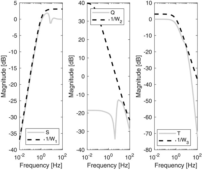
FIGURE 6. Bode magnitude plots of the sensitivity (S), the control sensitivity (Q) and the complementary sensitivity (T) functions. The dashed lines are the inverse of the weights used to shape the plant response. Multi-layer ${\mathcal{H}}_{\infty }$ case.

The reference pre-filter, F_ρ(s), generates the reference for the course rate loop. The reference depends on the curvature of the target path. Ideally $G_{{\varphi }_{ref}\to \varphi }(s)$, i.e., the transfer function from ϕ_ref to ϕ, should be 1. Thus, the simplest choice would be: $F_{\rho }(s)=G_{{\varphi }_{ref}\to \varphi }{(s)}^{-1}$. In practice, we are interested in having a unitary transfer function only up to a certain bandwidth; we assume that most manoeuvrers excite the course rate up to 1 Hz (Roselli et al., 2017). Thanks to this hypothesis, we approximate $G_{{\varphi }_{ref}\to \varphi }(s)$ as a time delay (Figure 7) which makes F_ρ(s) a time advance that provides the future reference course rate to the controller; no casualty issue arises since the trajectory is known in autonomous driving applications.

FIGURE 7

FIGURE 7. Bode plot of $G_{{\varphi }_{ref}\to \varphi }(s)$ (continuos) an its approximation (dashed).

The lateral error loop: finally, the external loop can be closed to guarantee a tracking also in the case of small errors in the course rate control. $K_{e_{cg}}(s)$ is tuned based on the transfer function from δ_e to e_cg in which the course rate loop is considered. The controller, tuned to guarantee null steady state error, yields a bandwidth of 0.47 Hz with a phase margin of 67°. For the sake of completeness, the gain of $K_{e_{cg}}(s)$ is scheduled according to the vehicle velocity:

$K_{e_{cg}}\left(0\right)=K_{e_{cg},90}\left(0\right)\frac{90/3.6}{v}(19)$

where $K_{e_{cg},90}$ is the controller transfer function tuned at 90 km/h.

In the following, the pre-filter and the lateral error controller are kept fixed for all the proposed configurations. Since the minimum bandwidth requirement is the same between the controllers, the higher levels do not need to be changed.

3.3 Q-LPV/${\mathcal{H}}_{\mathbf{\infty }}$ Course Rate Preview

The course rate controller considers a linear single-track model. When a vehicle performs emergency obstacle avoidance manoeuvrers, a linear model may not accurately describe the vehicle dynamics. If reliable estimations of the vehicle side slip angle and friction coefficient (as the one provided by Grip et al. (2008) are available, one can improve the performance and robustness of the controller by considering the tire nonlinearities in the design. The LPV framework provides a straightforward and systematic way to do so. Model (18) can be expressed as a q-LPV system by choosing the parameter vector

$p=\left[\frac{C_f\left({\alpha }_f\right)}{mv}\frac{C_f\left({\alpha }_f\right)l_f}{I_z}\frac{C_r\left({\alpha }_r\right)}{mv}\frac{C_r\left({\alpha }_r\right)l_r}{I_z}\right].(20)$

By linearizing the single-track around an arbitrary ${\bar{\alpha }}_{fr}$ we obtain:

$\begin{array}{c}\hfill \dot{x}=\left(A_0+A_1{p}_1+A_2{p}_2+A_3{p}_3+A_4{p}_4\right)x+\left(B_0+B_1{p}_1+B_2{p}_2+B_3{p}_3+B_4{p}_4\right)\tilde{u}+E\hfill \end{array}(21)$

where:

$\begin{array}{c}\hfill A_0=\left[\begin{array}{ccc}\hfill 0\hfill & \hfill -1\hfill & \hfill 0\hfill \\ \hfill 0\hfill & \hfill -\frac{k_p}{I_z}\hfill & \hfill \frac{k_i}{I_z}\hfill \\ \hfill 0\hfill & \hfill -1\hfill & \hfill 0\hfill \end{array}\right]A_1=\left[\begin{array}{ccc}\hfill -1\hfill & \hfill -\frac{l_f}{v}\hfill & \hfill 0\hfill \\ \hfill 0\hfill & \hfill 0\hfill & \hfill 0\hfill \\ \hfill 0\hfill & \hfill 0\hfill & \hfill 0\hfill \end{array}\right]A_2=\left[\begin{array}{ccc}\hfill 0\hfill & \hfill 0\hfill & \hfill 0\hfill \\ \hfill -1\hfill & \hfill -\frac{l_f}{v}\hfill & \hfill 0\hfill \\ \hfill 0\hfill & \hfill 0\hfill & \hfill 0\hfill \end{array}\right]\hfill \\ \hfill A_3=\left[\begin{array}{ccc}\hfill -1\hfill & \hfill \frac{l_r}{v}\hfill & \hfill 0\hfill \\ \hfill 0\hfill & \hfill 0\hfill & \hfill 0\hfill \\ \hfill 0\hfill & \hfill 0\hfill & \hfill 0\hfill \end{array}\right]A_4=\left[\begin{array}{ccc}\hfill 0\hfill & \hfill 0\hfill & \hfill 0\hfill \\ \hfill 1\hfill & \hfill -\frac{l_r}{v}\hfill & \hfill 0\hfill \\ \hfill 0\hfill & \hfill 0\hfill & \hfill 0\hfill \end{array}\right]\hfill \\ \hfill B_0=\left[\begin{array}{cc}\hfill 0\hfill & \hfill 0\hfill \\ \hfill 0\hfill & \hfill \frac{k_p}{I_z}\frac{v}{L+K_{usdes}{v}^2}\hfill \\ \hfill 0\hfill & \hfill \frac{v}{L+K_{usdes}{v}^2}\hfill \end{array}\right]B_1=\left[\begin{array}{cc}\hfill 1\hfill & \hfill 0\hfill \\ \hfill 0\hfill & \hfill 0\hfill \\ \hfill 0\hfill & \hfill 0\hfill \end{array}\right]B_2=\left[\begin{array}{cc}\hfill 0\hfill & \hfill 0\hfill \\ \hfill 1\hfill & \hfill 0\hfill \\ \hfill 0\hfill & \hfill 0\hfill \end{array}\right]B_3=\left[\begin{array}{cc}\hfill 0\hfill & \hfill 0\hfill \\ \hfill 0\hfill & \hfill 0\hfill \\ \hfill 0\hfill & \hfill 0\hfill \end{array}\right]B_4=\left[\begin{array}{cc}\hfill 0\hfill & \hfill 0\hfill \\ \hfill 0\hfill & \hfill 0\hfill \\ \hfill 0\hfill & \hfill 0\hfill \end{array}\right]\hfill \\ \hfill E=\left[\begin{array}{c}\hfill \frac{f_f\left({\bar{\alpha }}_f\right)+f_r\left({\bar{\alpha }}_r\right)+C_f{\bar{\alpha }}_f+C_r{\bar{\alpha }}_r}{mv}\hfill \\ \hfill \frac{l_f{f}_f\left({\bar{\alpha }}_f\right)-l_r{f}_r\left({\bar{\alpha }}_r\right)+l_f{C}_f{\bar{\alpha }}_f-l_r{C}_r{\bar{\alpha }}_r}{I_z}\hfill \\ \hfill 0\hfill \end{array}\right]\hfill \\ \hfill x=\left[\begin{array}{c}\hfill \beta \hfill \\ \hfill r\hfill \\ \hfill \zeta \hfill \end{array}\right]\tilde{u}=\left[\begin{array}{c}\hfill {\delta }_w\hfill \\ \hfill {\delta }_{wcmd}\hfill \end{array}\right].\hfill \end{array}$

Matrix E can be regarded as a constant input to the system that will be compensated by guaranteeing a high low frequency gain in the controller.

Some remarks concerning the choice of the parameters are due. Firstly, note that the actual physical scheduling parameters are the front and rear generalized cornering stiffnesses. However, in defining the LPV system, we have employed a larger parameter set. The combined parameter vector p has the advantage of better scaling the numerical range of the parameter variability thus improving the numerical properties of the resulting Linear Matrix Inequalities (LMI). By fixing as higher bounds (${\bar{C}}_{f,r}$) the cornering stiffnesses on dry asphalt and as lower bounds (${\underline{C}}_{f,r}$) their half, with the proposed solution p_1,3 range from 1 to 3 and p_2,4 from 50 to 100. If we had chosen p = [C_f(α_f) C_r(α_r)] the parameters would have spaced from to 10³ to 2 ⋅ 10³. By reducing the parameter variation magnitude, we obtain a more numerically robust problem that results in a lower performance index when numerically solved.

Secondly, we highlight the fact that there exists a trade-off between parameter set amplitude and performance. When it comes to decide the parameters range, one may be tempted to consider the absolute maximum and minimum values of the generalized cornering stiffnesses as bounds. It this way, all the possible system trajectories would have been considered. However, synthesizing a controller that stabilizes the system in all the theoretically reachable conditions would hardly satisfy the limitation imposed on the actuator usage generating an inadequate solution. Conversely, if we shrink too much the parameters space the advantages of scheduling vanishes.

The last remark regards the vehicle speed. We have decided to not schedule the system according to the velocity. Indeed, considering that its dynamics depend on the vehicle mass and the generalized cornering stiffness variation depends on $\frac{\partial f}{\partial \alpha }$, it is sensible to assume that the velocity varies slower than C_f,r and its impact can be accounted for with a slower and simpler controller scheduling. In the next section this issue will be further discussed.

Based on the above LPV model, we design a self-scheduled ${\mathcal{H}}_{\infty }$ controller using the same structure and weights rationale of the previous fixed structure controller. Figure 8 exemplifies the closed-loop transfer functions for a particular p. The pre-filter and the lateral error loop tuning are unchanged.

FIGURE 8

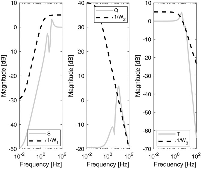
FIGURE 8. Bode magnitude plots of the sensitivity (S), the control sensitivity (Q) and the complementary sensitivity (T) functions. The q-LPV system has been evaluated for $\bar{p}=(\frac{3}{4}\frac{C_f}{mv},\frac{3}{4}\frac{C_f{l}_f}{I_z},\frac{3}{4}\frac{C_r}{mv},\frac{3}{4}\frac{C_r{l}_r}{I_z})$. The dashed lines are the inverse of the weights used to shape the plant response. Multi-layer q-LPV/${\mathcal{H}}_{\infty }$ case.

4 Validation and Discussion

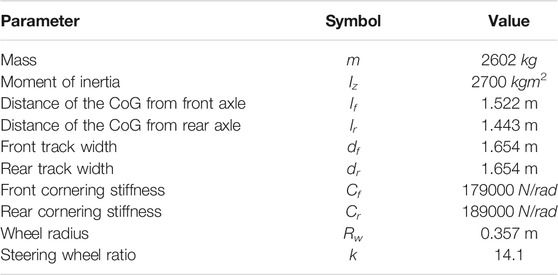
The analysis has been carried out in simulation exploiting IPG CarMaker², a multi-body vehicle simulation software. It considers critical elements such as tire nonlinear characteristics (Magic Formula 6.1), suspension dynamics and kinematics and load transfer phenomena. The controlled vehicle is a SUV with a 4WD drivetrain, Table 1 lists its main parameters.

TABLE 1

TABLE 1. Vehicle parameters.

In order to assess the course rate preview effectiveness a DLC manoeuvre is executed at different velocities and with different road friction coefficients. For a more objective analysis three performance indexes are considered:

• root mean square of the lateral error: $RM{S}_{e_{cg}}=\sqrt{\frac{1}{T}{\int }_0^T{e}_{cg}(\gamma )d\gamma }$;

• steering actuator usage: $SAU=\frac{1}{T}{\int }_0^T|{\delta }_{wcmd}(\gamma )|d\gamma$;

• yaw moment usage: $YMU=\frac{1}{T}{\int }_0^T|M_z(\gamma )|d\gamma$.

First of all, we analyze the behavior of the course rate preview. It is compared against a lateral controller based on Kapania and Gerdes (2015). The benchmark features a feedback contribution based on the look-ahead error and a feedforward term; TV is kept unchanged and active. The controller tuning minimizes the $RM{S}_{e_{cg}}$. Figure 9 shows a DLC on high grip at 80 km/h; which is within the vehicle handling limits. The figure plots the reference and executed trajectory, the course rate and the error at the centre of gravity. From the figure, one appreciates how the control scheme perfectly tracks the reference trajectory. The $RM{S}_{e_{cg}}$ of the multi-layer ${\mathcal{H}}_{\infty }$ is about 3 cm and the peak error is 10 cm. The benchmark solution shows a $RM{S}_{e_{cg}}$ of 7 cm and a peak error of 20 cm. The course rate preview working mechanism is well depicted in the course rate plot. The required course rate (dotted black) is fed in advance as reference (dashed black), thanks to the pre-filter the course rate loop lag is attenuated. The curvature preview term is more effective than the use of a look-ahead distance. Indeed, ϕ_{multi−layer} is in advance with respect to ϕ_benchmark.

FIGURE 9

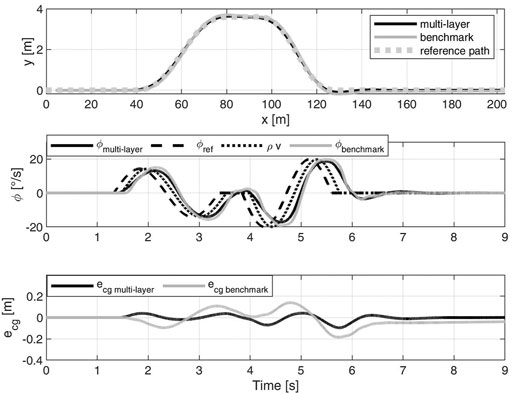
FIGURE 9. DLC at 80 km/h on μ = 1. Comparison between the multi-layer ${\mathcal{H}}_{\infty }$ and the proposed benchmark solution.

For a comprehensive analysis, the ${\mathcal{H}}_{\infty }$ and the q-LPV/${\mathcal{H}}_{\infty }$ are compared to an integrated approach. Thus, an additional controller is introduced as benchmark: a MISO q-LPV/${\mathcal{H}}_{\infty }$. Indeed, the multi-layer approach has the advantage of keeping the actuators management separated. This is convenient from the architecture point of view, but may be suboptimal from the performance standpoint. To design the integrated approach, many choices of the controllable outputs can be done. We decided to consider the system as multi-input ([δ_{w cmd}, M_z]) single-output ([ϕ]). The lateral error dynamics can be considered slower than the course rate one. Utilizing the same approach of the course rate preview: the inner loop, a MISO q-LPV/${\mathcal{H}}_{\infty }$, computes the steering angle and the yaw moment, the pre-filter and lateral error loop are left unchanged. The q-LPV/${\mathcal{H}}_{\infty }$ approach previously described has been integrated adding a weight on the yaw moment and the MISO q-LPV/${\mathcal{H}}_{\infty }$ controllers is synthesized.

Table 2 resumes the simulation results. We consider two manoeuvres both beyond the handling limits of the vehicle. The perfect tracking of the DLC at 100 km/h on high grip would require a maximal lateral acceleration of 12.4 m/s², the DLC on μ = 0.4 yields a peak lateral acceleration of 7.4 m/s². Given the tires limits, the maximal available lateral acceleration is 1 g and 0.4 g on high and low grip respectively. From the table, the following remarks are due:

• at 100 km/h, the multi-layer approaches maximize the usage of the yaw moment, fully exploiting the over-actuated architecture. The MISO q-LPV/${\mathcal{H}}_{\infty }$ exploits both the actuators, but its lateral error is beyond 20 cm. The multi-layer q-LPV/${\mathcal{H}}_{\infty }$ achieves the best performance considering all the indexes.

• at 80 km/h, despite the high steering wheel usage, the multi-layer approach keeps the vehicle stable. Comparing the q-LPV approaches, the MISO q-LPV/${\mathcal{H}}_{\infty }$ reaches slightly better performance. Anyway, by looking at the whole tests the multi-layer q-LPV/${\mathcal{H}}_{\infty }$ demonstrates a better average behavior.

TABLE 2

TABLE 2. Performance indexes of the DLC for different speeds and friction coefficients.

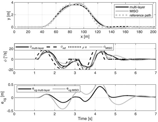
We analyze also the time domain behaviour of the controllers. Figure 10 shows the DLC at 100 km/h on high grip. In particular, we compare the multi-layer q-LPV/${\mathcal{H}}_{\infty }$ and MISO q-LPV/${\mathcal{H}}_{\infty }$ approaches. It is evident that the first one has better performance. From the course rate plot, it can be observed that the MISO controller has a lower bandwidth with respect to the multi-layer approach and struggles to follow the reference. Anyway, in the design of the MISO controller we have requested the same minima requirements. However, LMI solution returns a performance index of 10. Tuning the multi-input single-output controller is not straightforward. The complexity of the MISO setup effectively prevents it to attain its full potential.

FIGURE 10

FIGURE 10. DLC at 100 km/h on μ = 1. Multi-layer q-LPV/${\mathcal{H}}_{\infty }$ vs MISO q-LPV/${\mathcal{H}}_{\infty }$.

To discuss the validity of the hypothesis done to obtain the controller we further analyze the manoeuvre. First of all, the single-track model was derived with the hypothesis of small angles. From the top plot of Figure 11 it can be observed that the steering wheel angle at the wheels reaches non negligible values. Thus, the control is robust with respect to high steering commands. We highlight that the most critical non-linearity in the single-track mode is the tire linearization. Indeed, the bottom plot shows that we cover both the linear and nonlinear regions. Considering this behavior, as we did with LPV formulation, is paramount. Lastly, the comment about prioritizing the cornering stiffness scheduling with respect to the velocity is motivated. From the figure it is clear that the vehicle speed is varying slower than α_f,r, and as consequence slower than the generalized cornering stiffness. Thus, the velocity dependency is considered with more classical gain scheduling techniques, e.g. linearization scheduling (Rugh and Shamma, 2000).

FIGURE 11

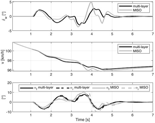
FIGURE 11. DLC at 100 km/h on μ = 1. Multi-layer q-LPV/${\mathcal{H}}_{\infty }$ vs MISO q-LPV/${\mathcal{H}}_{\infty }$. Detail of the steering wheel angle at the wheel, the vehicle velocity and the front/rear wheel slip angles.

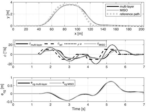
Figure 12 compares the multi-layer and MISO approaches on low grip. The interesting fact is that both approaches obtain a very similar behavior. Thus, the multi-layer strategy reaches the performance of an integrated method.

FIGURE 12

FIGURE 12. DLC at 80 km/h on μ = 0.4. Multi-layer q-LPV/${\mathcal{H}}_{\infty }$ vs MISO q-LPV/${\mathcal{H}}_{\infty }$.

Finally, Figure 13 shows the $RM{S}_{e_{cg}}$ of the DLCs for different lower bounds choice. As previously pointed out, there exists a trade-off between parameters range and performance. On one hand, the wider the parameters space the more difficult is the synthesis of the controller resulting in unsatisfactory performance. On the other hand, a narrow parameter space nullifies the effectiveness of the scheduling strategy, i.e., guarantee stability and leverage actuators peculiarities (this is evident from Table 2).

FIGURE 13

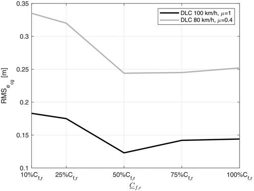
FIGURE 13. Sensitivity of the $RM{S}_{e_{cg}}$ with respect to the lower bounds of the parameters space (${\underline{C}}_{f,r}$). The lower bounds are expressed as a percentage of the nominal cornering stiffness.

5 Conclusion

In this paper, we have proposed a multi-layer q-LPV/${\mathcal{H}}_{\infty }$ control scheme. The multi-layer approach, separating the actuators management, exploits possible pre-existing control systems and simplifies the design process. We highlight the fact that the multi-layer course rate preview is aware of the underlying TV system since it is considered in the tuning process. Furthermore, it has been compared to MISO technique demonstrating excellent performance.

Besides, the introduction of tire nonlinearities, exploiting LPV formulation, proved to increase the conditions in which a DLC is feasible. The choice of the parameters and their range have been discussed.

The next steps consist in introducing the velocity as an additional scheduling variable and validating experimentally the proposed strategies.

Data Availability Statement

The original contributions presented in the study are included in the article/Supplementary Material, further inquiries can be directed to the corresponding author.

Author Contributions

AG contributed to the design of control law, simulation and writing of the original draft. MC helped with the methodology, guidance, review and editing. SS helped with review and editing. All authors contributed to the article and approved the submitted version.

Conflict of Interest

The authors declare that the research was conducted in the absence of any commercial or financial relationships that could be construed as a potential conflict of interest.

Publisher’s Note

All claims expressed in this article are solely those of the authors and do not necessarily represent those of their affiliated organizations, or those of the publisher, the editors, and the reviewers. Any product that may be evaluated in this article, or claim that may be made by its manufacturer, is not guaranteed or endorsed by the publisher.

Footnotes

¹usually, the term cornering stiffness refers to the linearized curve for α = 0

²https://ipg-automotive.com/

References

Abe, M. (2015). Vehicle Handling Dynamics: Theory and Application. Butterworth-Heinemann.

Google Scholar

Alcalá, E., Puig, V., Quevedo, J., and Escobet, T. (2017). Gain Scheduling Lpv Control Scheme for the Autonomous Guidance Problem Using a Dynamic Modelling Approach. London: IET. https://arxiv.org/abs/1712.00390.

Google Scholar

Amer, N. H., Zamzuri, H., Hudha, K., and Kadir, Z. A. (2017). Modelling and Control Strategies in Path Tracking Control for Autonomous Ground Vehicles: A Review of State of the Art and Challenges. J. Intell. Robot Syst. 86, 225–254. doi:10.1007/s10846-016-0442-0

CrossRef Full Text | Google Scholar

Beal, C. E., and Gerdes, J. C. (2013). Model Predictive Control for Vehicle Stabilization at the Limits of Handling. IEEE Trans. Contr. Syst. Technol. 21, 1258–1269. doi:10.1109/TCST.2012.2200826

CrossRef Full Text | Google Scholar

Chatzikomis, C., Sorniotti, A., Gruber, P., Zanchetta, M., Willans, D., and Balcombe, B. (2018). Comparison of Path Tracking and Torque-Vectoring Controllers for Autonomous Electric Vehicles. IEEE Trans. Intell. Veh. 3, 559–570. doi:10.1109/TIV.2018.2874529

CrossRef Full Text | Google Scholar

Corno, M., Panzani, G., Roselli, F., Giorelli, M., Azzolini, D., and Savaresi, S. M. (2021). An Lpv Approach to Autonomous Vehicle Path Tracking in the Presence of Steering Actuation Nonlinearities. IEEE Trans. Contr. Syst. Technol. 29, 1766–1774. doi:10.1109/TCST.2020.3006123

CrossRef Full Text | Google Scholar

De Novellis, L., Sorniotti, A., Gruber, P., and Pennycott, A. (2014). Comparison of Feedback Control Techniques for Torque-Vectoring Control of Fully Electric Vehicles. IEEE Trans. Veh. Technol. 63, 3612–3623. doi:10.1109/tvt.2014.2305475

CrossRef Full Text | Google Scholar

Fagnant, D. J., and Kockelman, K. (2015). Preparing a Nation for Autonomous Vehicles: Opportunities, Barriers and Policy Recommendations. Transportation Res. A: Pol. Pract. 77, 167–181. doi:10.1016/j.tra.2015.04.003

CrossRef Full Text | Google Scholar

Falcone, P., Borrelli, F., Asgari, J., Tseng, H. E., and Hrovat, D. (2007). Predictive Active Steering Control for Autonomous Vehicle Systems. IEEE Trans. Contr. Syst. Technol. 15, 566–580. doi:10.1109/TCST.2007.894653

CrossRef Full Text | Google Scholar

Falcone, P., Eric Tseng, H., Borrelli, F., Asgari, J., and Hrovat, D. (2008). Mpc-based Yaw and Lateral Stabilisation via Active Front Steering and Braking. Vehicle Syst. Dyn. 46, 611–628. doi:10.1080/00423110802018297

CrossRef Full Text | Google Scholar

Fergani, S., Sename, O., and Dugard, L. (2016). An LPV/H∞ Integrated Vehicle Dynamic Controller Integrated Vehicle Dynamic Controller. IEEE Trans. Veh. Technol. 65, 1880–1889. doi:10.1109/TVT.2015.2425299

CrossRef Full Text | Google Scholar

Fiala, E. (1954). Seitenkraften am rollenden Luftreifen. VdI 96, 973–979.

Google Scholar

Frieske, B., Kloetzke, M., and Mauser, F. (2013). “Trends in Vehicle Concept and Key Technology Development for Hybrid and Battery Electric Vehicles,” in 2013 World Electric Vehicle Symposium and Exhibition (EVS27), Barcelona, Spain, November 17–20, 2013, 1–12. doi:10.1109/evs.2013.6914783

CrossRef Full Text | Google Scholar

Goodarzi, A., Sabooteh, A., and Esmailzadeh, E. (2008). Automatic Path Control Based on Integrated Steering and External Yaw-Moment Control. Proc. Inst. Mech. Eng. K: J. multi-body Dyn. 222, 189–200. doi:10.1243/14644193jmbd120

CrossRef Full Text | Google Scholar

Grip, H. F., Imsland, L., Johansen, T. A., Fossen, T. I., Kalkkuhl, J. C., and Suissa, A. (2008). Nonlinear Vehicle Side-Slip Estimation with Friction Adaptation. Automatica 44, 611–622. doi:10.1016/j.automatica.2007.06.017

CrossRef Full Text | Google Scholar

Guo, N., Zhang, X., Zou, Y., Lenzo, B., and Zhang, T. (2020). A Computationally Efficient Path-Following Control Strategy of Autonomous Electric Vehicles with Yaw Motion Stabilization. IEEE Trans. Transp. Electrific. 6, 728–739. doi:10.1109/TTE.2020.2993862

CrossRef Full Text | Google Scholar

Harkegard, O. (20022002). Efficient Active Set Algorithms for Solving Constrained Least Squares Problems in Aircraft Control Allocation. Proc. 41st IEEE Conf. Decis. Control. 2, 1295–1300. doi:10.1109/CDC.2002.1184694

CrossRef Full Text | Google Scholar

Huang, K., Yang, X., Lu, Y., Mi, C. C., and Kondlapudi, P. (2018). Ecological Driving System for Connected/automated Vehicles Using a Two-Stage Control Hierarchy. IEEE Trans. Intell. Transport. Syst. 19, 2373–2384. doi:10.1109/tits.2018.2813978

CrossRef Full Text | Google Scholar

Kaiser, G., Liu, Q., Hoffmann, C., Korte, M., and Werner, H. (2014). Lpv Torque Vectoring for an Electric Vehicle with Experimental Validation. IFAC Proc. Volumes 47, 12010–12015. 19th IFAC World Congress. doi:10.3182/20140824-6-ZA-1003.00163

CrossRef Full Text | Google Scholar

Kapania, N. R., and Gerdes, J. C. (2015). Design of a Feedback-Feedforward Steering Controller for Accurate Path Tracking and Stability at the Limits of Handling. Vehicle Syst. Dyn. 53, 1687–1704. doi:10.1080/00423114.2015.1055279

CrossRef Full Text | Google Scholar

Katriniok, A., Maschuw, J. P., Christen, F., Eckstein, L., and Abel, D. (2013). “Optimal Vehicle Dynamics Control for Combined Longitudinal and Lateral Autonomous Vehicle Guidance,” in 2013 European Control Conference (ECC), Orlando, FL, December 12–15, 2011, 974–979. doi:10.23919/ecc.2013.6669331

CrossRef Full Text | Google Scholar

Kiencke, U., and Nielsen, L. (2000). Automotive Control Systems: For Engine, Driveline, and Vehicle. Heidelberg: Springer.

Google Scholar

Li, P., Nguyen, A.-T., Du, H., Wang, Y., and Zhang, H. (2021). Polytopic Lpv Approaches for Intelligent Automotive Systems: State of the Art and Future Challenges. Mech. Syst. Signal Process. 161, 107931. doi:10.1016/j.ymssp.2021.107931

CrossRef Full Text | Google Scholar

Liniger, A., Domahidi, A., and Morari, M. (2017). Optimization-based Autonomous Racing of 1: 43 Scale Rc Cars. ArXiv abs/1711.07300.Hoboken, NJ: Wiley

Google Scholar

Lucchini, A., Formentin, S., Corno, M., Piga, D., and Savaresi, S. M. (2020). Torque Vectoring for High-Performance Electric Vehicles: An Efficient Mpc Calibration. IEEE Control. Syst. Lett. 4, 725–730. doi:10.1109/LCSYS.2020.2981895

CrossRef Full Text | Google Scholar

Mohammadpour, J., and Scherer, C. W. (2012). Control of Linear Parameter Varying Systems with Applications. Springer Science & Business Media.

Google Scholar

Németh, B., Gáspár, P., and Bokor, J. (2016). “Lpv-based Integrated Vehicle Control Design Considering the Nonlinear Characteristics of the Tire,” in 2016 American Control Conference (ACC), Boston: IEEE, 6893–6898. doi:10.1109/ACC.2016.7526758

CrossRef Full Text | Google Scholar

Pacejka, H. (2005). Tire and Vehicle Dynamics. Elsevier.

Google Scholar

Peng, H., Wang, W., An, Q., Xiang, C., and Li, L. (2020). Path Tracking and Direct Yaw Moment Coordinated Control Based on Robust Mpc with the Finite Time Horizon for Autonomous Independent-Drive Vehicles. IEEE Trans. Veh. Technol. 69, 6053–6066. doi:10.1109/TVT.2020.2981619

CrossRef Full Text | Google Scholar

Peters, S., Frazzoli, E., and Iagnemma, K. (20112011). Differential Flatness of a Front-Steered Vehicle with Tire Force Control. IEEE/RSJ Int. Conf. Intell. Robots Syst., 298–304. doi:10.1109/iros.2011.6094800

CrossRef Full Text | Google Scholar

Rajamani, R. (2011). Vehicle Dynamics and Control. Springer US. Mechanical Engineering Series.

Google Scholar

Roselli, F., Corno, M., Savaresi, S. M., Giorelli, M., Azzolini, D., Irilli, A., and Panzani, G. (2017). “H∞ Control with Look-Ahead for Lane Keeping in Autonomous Vehicles,” in 2017 IEEE Conference on Control Technology and Applications (CCTA), Kohala Coast, Hawaii, August 27–30, 2017, 2220–2225. doi:10.1109/CCTA.2017.8062781

CrossRef Full Text | Google Scholar

Rossetter, E. J., Switkes, J., and Gerdes, J. C. (2004). Experimental Validation of the Potential Field Lanekeeping System. Int. J. Automotive Technol. 5, 95–108. doi:10.1109/ACC.2003.1240417

CrossRef Full Text | Google Scholar

Rugh, W. J., and Shamma, J. S. (2000). Research on Gain Scheduling. Automatica 36, 1401–1425. doi:10.1016/S0005-1098(00)00058-3

CrossRef Full Text | Google Scholar

Skogestad, S., and Postlethwaite, I. (2007). Multivariable Feedback Control: Analysis and Design, Vol. 2. Hoboken, NJ: Wiley.

Google Scholar

Stogios, C., Kasraian, D., Roorda, M. J., and Hatzopoulou, M. (2019). Simulating Impacts of Automated Driving Behavior and Traffic Conditions on Vehicle Emissions. Transportation Res. D: Transport Environ. 76, 176–192. doi:10.1016/j.trd.2019.09.020

CrossRef Full Text | Google Scholar

Tagne, G., Talj, R., and Charara, A. (2013). “Higher-order Sliding Mode Control for Lateral Dynamics of Autonomous Vehicles, with Experimental Validation,” in 2013 IEEE Intelligent Vehicles Symposium (IV), Gold Coast, Australia, June 23–26, 2013, 678–683. doi:10.1109/IVS.2013.6629545

CrossRef Full Text | Google Scholar

Yakub, F., and Mori, Y. (2015). Comparative Study of Autonomous Path-Following Vehicle Control via Model Predictive Control and Linear Quadratic Control. Proc. Inst. Mech. Eng. D: J. automobile Eng. 229, 1695–1714. doi:10.1177/0954407014566031

CrossRef Full Text | Google Scholar

Zinnari, F., Strada, S., Tanelli, M., Formentin, S., Savaia, G., and Savaresi, S. M. (2020). “Mining the Electrification Potential of Fuel-Based Vehicles Mobility Patterns: a Data-Based Approach,” in 2020 IEEE International Conference on Human-Machine Systems (ICHMS), September 7–9, 2020, 1–S. doi:10.1109/ICHMS49158.2020.9209557

CrossRef Full Text | Google Scholar