Time and Action Co-Training in Reinforcement Learning Agents

In formation control, a robot (or an agent) learns to align itself in a particular spatial alignment. However, in a few scenarios, it is also vital to learn temporal alignment along with spatial alignment. An effective control system encompasses flexibility, precision, and timeliness. Existing reinforcement learning algorithms excel at learning to select an action given a state. However, executing an optimal action at an appropriate time remains challenging. Building a reinforcement learning agent which can learn an optimal time to act along with an optimal action can address this challenge. Neural networks in which timing relies on dynamic changes in the activity of population neurons have been shown to be a more effective representation of time. In this work, we trained a reinforcement learning agent to create its representation of time using a neural network with a population of recurrently connected nonlinear firing rate neurons. Trained using a reward-based recursive least square algorithm, the agent learned to produce a neural trajectory that peaks at the “time-to-act”; thus, it learns “when” to act. A few control system applications also require the agent to temporally scale its action. We trained the agent so that it could temporally scale its action for different speed inputs. Furthermore, given one state, the agent could learn to plan multiple future actions, that is, multiple times to act without needing to observe a new state.

1 Introduction

A powerful formation control system requires continuously monitoring the current state, comparing the performance, and deciding whether to take necessary actions. This process does not only need to understand the system’s state and optimal actions but also needs to learn the appropriate time to perform an action. Deep reinforcement learning algorithms which have achieved remarkable success in the field of robotics, games, and board games have also been shown to perform well in adaptive control system problems Li et al. (2019); Oh et al. (2015); Xue et al. (2013). However, the challenge of learning the precise time to act has not been directly addressed.

The ability to measure time from the start of a state change and use it accordingly is an essential part of applications such as adaptive control systems. In general, the environment encodes as four dimensions: the three dimensions of space and the dimension. The role of representation of time affects the decision-making process along with the spatial aspects of the environment Klapproth (2008). However, in the field of reinforcement learning (RL), the essential role of time is not explicitly acknowledged, and existing RL research mainly focuses on the spatial dimensions. The lack of time sense might not be an issue when considering a simple behavioral task, but many tasks in control systems require precisely timed actions for which an artificial agent is required to learn the representation of time and experience the passage of time.

Research on time representation has yielded several different supervised learning models such as the ramping firing rate Durstewitz (2003), multiple oscillator models Matell et al. (2003); Miall (1989), diffusion models Simen et al. (2011), and the population clock model Buonomano and Laje (2011). In some of these models, such as the two presented in the studies by Hardy et al. (2018) and Laje and Buonomano (2013), timing relies on dynamic changes in the activity patterns of neuron populations. More specifically, it relies on nonlinear firing rate neurons connected recurrently, and research has shown that these models are the most effective Buonomano and Laje (2011) and the best at accounting for timing and temporal scaling compared to other available models. Extending this work on a rote sense of time for agents, we used a population clock model recurrent neural network (RNN) consisting of nonlinear firing rate neurons as our timing module and trained a reinforcement learning agent to create its own representation of time.

It is arguable that a traditional artificial neural network, such as a multilayer perceptron, which was proven to learn complex spatial patterns, could also be used to learn time representation. However, these networks might not be well suited to perform a simple interval-discrimination task, due to the lack of the implicit representation of time Buonomano and Maass (2009). One argument is that a traditional artificial neural network processes inputs and outputs as a static spatial pattern. However, to achieve an effective control system, the agent needs to continuously process the state of the system. For instance, if we want an agent to process continuous-time input, such as a video in a game, we divide the input into multiple time-bins. Similarly, deep neural network (DNN) models with long short-term memory (LSTM) units Hochreiter and Schmidhuber (1997) or gated recurrent units (GRUs) Chung et al. (2014) can implicitly represent time by allowing the state of the previous time step to interact with the state of the current time step. These networks still treat time as a spatial dimension because they expect the input to be discretised into multiple time bins Bakker (2002)Buonomano and Maass (2009). Because these networks treat time as a spatial dimension, they might lack explicit time representation.

Through the lens of RL algorithms, the problem of discretising input into multiple time bins can be explained as follows. Given the current state of the environment $S_t$, a DNN function approximator (for example, a policy network) outputs an action at $A_t$ at every time step t. If an action $A_t$ is more valuable when executed at time $t+\delta x$ or $t-\delta y$, then to effectively maximize the summation of future rewards, we should further divide the input into smaller time steps. By dividing these time steps more finely, an agent could learn the true value of the state, although at the expense of a higher computation cost and with increased state value variance Petter et al. (2018). A few studies Carrara et al. (2019); Tallec et al. (2019); Doya (2000) have elegantly extended reinforcement learning algorithms to continuous time and state space, which generalizes the value function approximators over time. However, if an agent has developed a representation of the time, it could learn to explicitly encode the optimal time intervals itself and in turn, learn to decide when to act. In this study, we present the model of how the time representation is learned and the subsequent encoding process could take place.

In this research, we have developed a new scenario called “task switching,” where an agent is presented with multiple circles to click (task), and each circle should be clicked within a specific time window in a specific order. This scenario attempts to encapsulate both spatial and timing decisions. This task was built analogous to a multi-input multi-output (MIMO) system in process control tasks, where the system should compare the state of the current system and decide when making parameter changes to the system.

This research aims to investigate the co-learning of decision making and development of timing by an artificial agent using a reinforcement learning framework. We achieve this by disentangling the process of learning optimal action (which circle to click) and time representation (when to click a circle). We designed a novel architecture that contains two modules: 1. a timing module that uses a population clock model, a recurrent neural network (RNN) consisting of nonlinear firing rate neurons, and 2. an action module that employs a deep Q-network (DQN) Mnih et al. (2015) to learn the optimal action given a specific state. The RNN and DQN are co-trained to learn the time to act and action. The RNN was trained using a reward-based recursive least squares algorithm, and the DQN was trained using the Bellman equation. The results of a series of task-switching scenarios show that the agent learned to produce a neural trajectory reflecting its own sense of time that peaked at the correct time-to-act. Furthermore, the agent was able to temporally scale its time-to-act more quickly or more slowly according to the input speed. We also compared the performance of the proposed architecture with DNN models such as LSTM, which can implicitly represent time. We observed that for tasks involving precisely timed action, neural network models such as the population clock model perform better than the LSTM.

This article first presents the task-switching scenario and describes the proposed architecture and training methodology used in the work. Section 3 presents the performance of the trained RL agent on six different experiments. In Section 4, we present the performance of LSTM in comparison with the proposed model. Finally, Section 5 presents an extensive discussion about the learned time representation with respect to prior electrophysiology studies.

2 Methods

2.1 Task-Switching Scenario

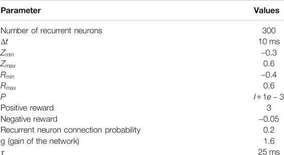
In the scenario, there are n different circles, and the agent must learn to click on each circle within a specific time interval and in a specific order. This task involves learning to decide which circle to click and when that circle should be clicked. Figure 1 shows an example scenario with four circles. Circle 1 must be clicked at some point between 800 and 900 ms. Similarly, circles 2, 3, and 4 must be clicked at 1,500–1,600, 2,300–2,400, and 3,300–3,400 ms, respectively. If the agent clicks the correct circle in the correct time period, it receives a positive reward. If it clicks a circle at the incorrect time, it receives a negative reward (refer to Table 1 for the exact reward values). Each circle becomes inactive once its time interval has passed. For example, circle 1 in Figure 1 becomes inactive at 901 ms, meaning that the agent cannot click it after 900 ms and receives a reward of 0 if it attempts to click the inactive circle. Each circle can only be clicked once during an episode.

FIGURE 1

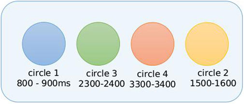
FIGURE 1. Task-switching scenario with four circles. Circle 1 (in blue) must be clicked at a time point between 800 and 900 ms from the start of the experiment. Circles 2 (in green), 3 (in orange), and 4 (in yellow) must be clicked in the 2,300–2,400, 3,300–3,400, and 1,500–1,600 ms intervals, respectively.

TABLE 1

TABLE 1. Model parameters.

The same scenario was modified to conduct the following experiments:

• Co-training time and action in a reinforcement learning agent on a simple task-switching scenario.

• Temporal scaling: the time intervals of each circle occur at different speeds. For instance, at Speed 2, circle 1 in Figure 1 must be clicked between 750 and 850 ms; similarly, circles 2, 3, and 4 must be clicked at 1,450–1,550, 2,250–2,350, and 3,250–3,350 ms, respectively.

• Multiple clicks: one circle should be clicked multiple times without any external cue. For instance, after circle 1 is clicked and without any further stimulus input, the agent should learn to click the same circle after a fixed time interval.

• Twenty circles: To understand if the agent can handle a large number of tasks, we trained the agent on a scenario containing 20 circles.

• Skip state: in the task-switching scenario, the learned time-to-act should be a state-dependent action. In other words, when the state input is eliminated, the agent should not perform an action. For instance, if circle 4 in Figure 1 is removed from the state input, the agent should skip clicking on circle 4.

2.2 Framework

To disentangle the learning of temporal and spatial aspects of the action space, the temporal aspect being when to act and the spatial being what to act on, we used two different networks: a DQN to learn which action to take and an RNN which learns to produce a neural trajectory that peaks at the time-to-act.

2.2.1 Deep Q-Network

In recent years, RL algorithms have given rise to tremendous achievements Vinyals et al. (2019); Mnih et al. (2013); Silver et al. (2017). RL manifests as a Markov decision process (MDP) defined by the state space $\mathcal{S}$, the action space $\mathcal{A}$, and the reward function $\mathrm{ℛ}:\mathcal{S}\times \mathcal{A}\to \mathrm{ℝ}$. At any given time step t, the agent receives a state $s_t\in \mathcal{S}$, which it uses to select an action $a_t\in \mathcal{A}$ and execute that action on the environment. Next, the agent receives a reward $r_{t+\delta t}\in \mathrm{ℛ}$, and the environment changes from state $s_t$ to $s_{t+\delta t}\in \mathcal{S}$. For each action the agent performs on the environment, it collects $\left(s_t,a_t,r_{t+\delta t},s_{t+\delta t}\right)$, also called an experience tuple. An agent learns to take actions that maximize the accumulated future rewards, which can be expressed as $R_t$ as follows:

$R_t={\displaystyle \sum _{t=1}^{\infty }{\gamma }^t{r}_t}(1)$

where $\gamma \mathit{ϵ}\left[\mathrm{0,1}\right]$ is the discount factor that determines the importance of the immediate reward and the future reward. If $\gamma =0$, the agent will learn to choose actions that produce an immediate reward. If $\gamma =1$, the agent will evaluate its actions based on the sum of all its future rewards. To learn the sequence of actions that lead to the maximum discounted sum of future rewards, an agent estimates optimal values for all possible actions in a given state. These estimated values are defined by the expected sum of future rewards under a given policy π.

$Q^{\pi }\left(s,a\right)=E_{\pi }\left\{R_t/s_t=s,a_t=a\right\}(2)$

where $E_{\pi }$ is the expectation under the policy π, and $Q^{\pi }\left(s,a\right)$ is the expected sum of discounted rewards when the action a is chosen by the agent in the state s under a policy π. Q-learning Watkins and Dayan (1992) is a widely used reinforcement learning algorithm that enables the agent to update its $Q^{\pi }\left(s,a\right)$ estimation iteratively by using the following formula:

$Q^{\pi }\left(s_t,a_t\right)=Q^{\pi }\left(s_t,a_t\right)+\alpha \left(r_t+\left(\gamma \max Q^{\pi }\left(s_{t+\delta t},a\right)-Q^{\pi }\left(s_t,a_t\right)\right)\right)(3)$

where α is the learning rate, and $Q^{\pi }\left(s_{t+1},a\right)$ is the future value estimate. By iteratively updating the Q values based on the agent’s experience, the Q function can be converged to the optimal Q function, which satisfies the following Bellman optimality equation:

$Q^{{\pi }^{\text{*}}}\left(s,a\right)=E\left\{r_t+\gamma \text{max}{Q}^{{\pi }^{\text{*}}}\left(s\prime ,a\prime \right)\right\}(4)$

where ${\pi }^{\text{*}}$ is the optimal policy. Action a can be determined as follows:

$a={\text{argmax}}_a{Q}^{\text{*}}\left(s,a\right)(5)$

When the state space and the action space are discrete and finite, the Q function can be a table that contains all possible state-action values. However, when the state and action spaces are large or continuous, a neural network is commonly used as a Q-function approximator Mnih et al. (2015); Lillicrap et al. (2015). In this work, we model a reinforcement learning agent which uses a fully connected DNN as a Q-function approximator to select one of the four circles.

2.2.2 Recurrent Neural Network

In this study, we used the population clock model for training the RL agent to learn the representation of time. In previous studies, this model has been shown to robustly learn and generate simple-to-complex temporal patterns Laje and Buonomano (2013); Hardy et al. (2018). The population clock model (i.e., RNN) contains a pool of recurrently connected nonlinear firing rate neurons with random initial weights as shown at the top of Figure 2. To achieve “time-to-act” and temporal scaling of timing behavior, we trained the weights of both recurrent neurons and output neurons. The network we used in this study contained 300 recurrent neurons, as indicated by the blue neurons inside the green circle, plus one input and one output neuron. The dynamics of the network Sompolinsky et al. (1988) are governed by Eqs 6–8. The learning showed a similar performance on a larger number of neurons, and the performance started to decline when 200 neurons were used.

$\tau \frac{\text{d}{x}_i}{\text{d}t}=-x_i\left(t\right)+{\displaystyle \sum _{j=1}^N{W}_{ij}^{\text{Rec}}f{r}_j\left(t\right)}+{\displaystyle \sum _{j=1}^I{W}_{ij}^{\text{In}}{y}_j\left(t\right)}(6)$

$z={\displaystyle \sum _{j=1}^N{W}_j^{\text{Out}}{r}_j}(7)$

$f{r}_i=\text{tanh}\left(x_i\right)(8)$

FIGURE 2

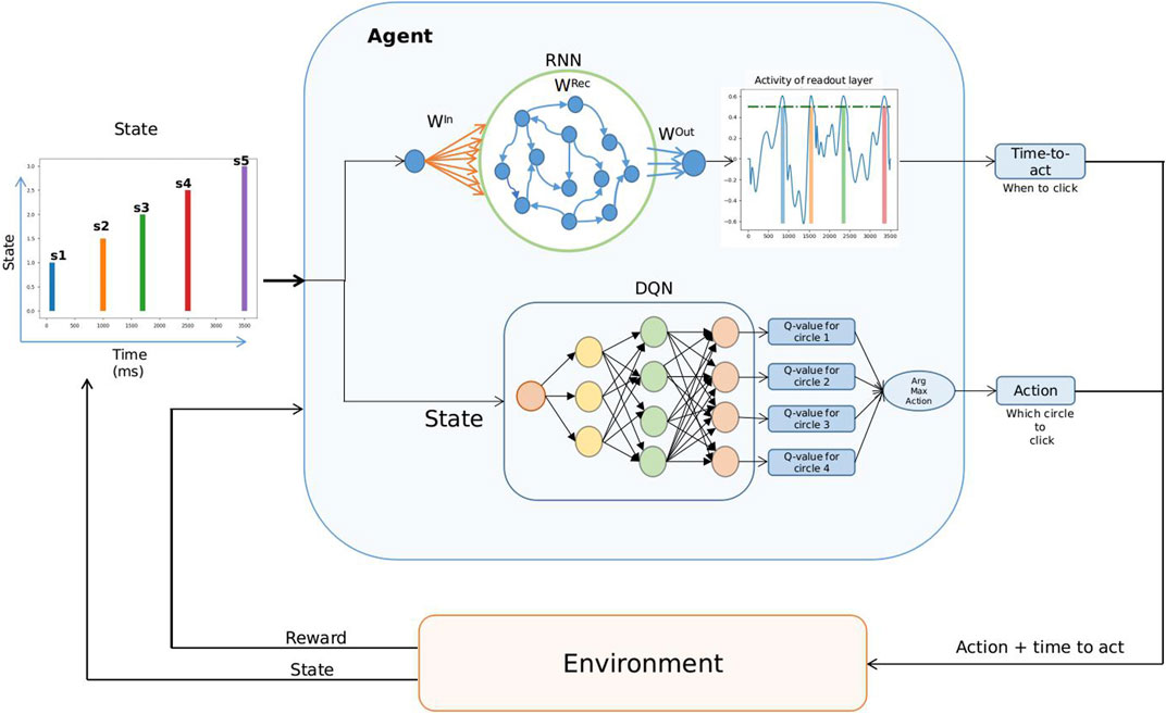
FIGURE 2. Proposed reinforcement learning architecture. (A) State input is received by the agent over an episode with a length of 3,600 ms. The agent contains an RNN (B) and a deep Q-network (C). The RNN receives a continuous input signal with state values for 20 ms and zeros for the remaining time. The state values shown here are $s1=1.0$, $s2=1.5$, $s3=2.0$, $s4=2.5$, and $s5=3$. The weights $W^{\text{ln}}$ (the orange connections) are initialized randomly and held constant throughout the experiment. The weights $W^{\text{Rec}}$ and $W^{out}$ (the blue connections) are initialized randomly and trained over the episodes. The DQN with one input and four output nodes receives the state value as its input and outputs the Q-value for each circle.

Given a network that contains N recurrent neurons, $f{r}_i$ represents the firing of the $i^{th}=[\mathrm{1,2...},N]$ recurrent neuron. $W^{\text{Rec}}$, which is an $NxN$ weight matrix, defines the connectivity of the recurrent neurons, which is initialized randomly from a normal distribution with a mean of 0 and a standard deviation of $1/\sqrt{g\ast N}$, where g represents the gain of the network. Each input neuron is connected to every recurrent neuron in the network with a $W^{\text{ln}}$, which is an $Nx1$ input weight matrix. $W^{\text{ln}}$ is initialized randomly from a normal distribution with a mean of 0 and a standard deviation of 1 and is fixed during training. Similarly, every recurrent neuron is connected to each output neuron with a $W^{out}$, which is a $1xN$ output weight matrix. In this study, we trained $W^{\text{Rec}}$ and $W^{out}$ using a reward-based recursive least squares method. The variable y represents the activity level of the input neurons (states), and z represents the output. $x_i\left(t\right)$ represents the state of the $i^{th}$ recurrent neuron, which is initially zero, and τ is the neuron time constant.

Initially, due to the high gain caused by $W^{\text{Rec}}$ (when $g=1.6$), the network produces chaotic dynamics, which in theory can encode time for a long time Hardy et al. (2018). In practice, the recurrent weights need to be tuned to reduce this chaos and locally stabilize the output activity. The parameters, such as connection probability, $\text{Δ}t$, g (gain of the network), and τ, were chosen based on the existing population clock model research Buonomano and Maass (2009); Laje and Buonomano (2013). In this work, we trained both recurrent and output weights using a reward-based recursive least square algorithm. During an episode, the agent chooses to act when the output activity exceeds a threshold (in this study, 0.5). We experimented with other threshold values between 0.4 and 1, but each produced similar results to 0.5. If the activity never exceeds a threshold, then the agent chooses a random time point to act. This is to ensure that the agent tries different time points and acts before it learns the temporal nature of the task.

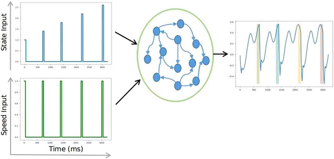
As illustrated in Figure 2 (left side), a sequence of state inputs are given to an agent during an episode lasting 3,600 ms, where each state for the RNN network is a 20-ms input signal and a single value for the DQN. The agent receives state $s1$ at $0ms$. At this point, all circles are active. At $900ms$, the first circle turns inactive, and the agent receives state $s_2$. In other words, the agent only receives the next state after the previous state has changed. In this case, the changes are caused by the circle turning inactive due to time constraints preset in the task. The final state, $s5$, is a terminal state where all the circles are inactive. Note that each action given by the Q network is only executed at the time points defined by the RNN network.

2.3 Time and Action Co-Training in Reinforcement Learning Agent

At the start of an episode, an agent explores the environment by selecting random circles to click. At the end of the episode, the agent collects a set of different experience tuples $\left(s_t,a_t,r_{t+\delta t},s_{t+\delta t}\right)$ that are used to train the DQN and RNN.

2.3.1 DQN

The parameters of the Q network θ are iteratively updated using Eqs. 9, 10 for action $a_t$ taken in state $s_t$, which results in reward $r_{t+\delta t}$.

${\theta }_{t+1}={\theta }_t+\alpha \left(y-Q\left(s_t,a_t;{\theta }_t\right)\right){\nabla }_{{\theta }_t}Q\left(a_t,a_t;{\theta }_t\right)(9)$

$y=r_{t+1}+\gamma \underset{t}{\text{max}}Q\left(s_{t+1},a;{\theta }_t\right)(10)$

2.3.2 Recurrent Neural Network

In the RNN, both the recurrent weights and output weights were updated at every $\text{Δ}t=10ms$, using the collected experiences. The recursive least square algorithm (RLS) Åström and Wittenmark (2013) is a basic recursive application of the least square algorithm. Given an input signal ${\text{x}}_1,{\text{x}}_2,\dots .{\text{x}}_{\text{n}}$ and the set of desired responses ${\text{y}}_1,{\text{y}}_2,\dots .{\text{y}}_{\text{n}}$, the RLS updates the parameters $W^{\text{Rec}}$ and $W^{\text{Out}}$ to minimize the mean difference between the desired and the actual output of the RNN (which is the firing rate $f{r}_i$ of the recurrent neuron). In the proposed architecture, we generate the desired response of recurrent neurons by adding a reward to the firing rate $f{r}_i\left(t\right)$ neuron i at time t such that the desired firing rate decreases at time t if $r_t<0$ and increases if $r_t>0$. The desired response of output neurons was generated by adding a reward to output activity z, as defined in Eq 7.

The error $e_i^{rec}\left(t\right)$ of recurrent neurons is computed using Eq 12, where $f{r}_i\left(t\right)$ is the firing rate of neuron i at time t, and $r_t$ is the reward received at time t. The desired signal $r_i\left(t\right)+reward\left(t\right)$ is clipped between $R_{min}$ and $R_{max}$ due to the high variance of the firing rate. The update of parameters $W^{\text{Rec}}$ is dictated by Eq 11, where $W_{ij}^{\text{Rec}}$ is the recurrent weight between the $i^{th}$ neuron and the $j^{th}$ neuron. The exact values of $Z_{min},Z_{max},R_{min}and{R}_{max}$ are shown in Table 1. $Z_{min}$ and $Z_{max}$ act as clamping values of the desired output activity. So, in this study, the value of $Z_{max}$ was chosen to be close to the positive threshold (+0.5), and the value of $Z_{min}$ was chosen to be close to the negative threshold (−0.5). The parameter $\text{Δ}t$ was set based on the existing population clock model research Buonomano and Maass (2009); Laje and Buonomano (2013).

In this study, we trained only a subset of recurrent neurons, which were randomly selected at the start of training. $SubRec$ is a subset of randomly selected neurons from the population. For the experiments in this study, we selected $30\text{\%}$ of the recurrent neurons for training. The square matrix ${\mathit{P}}^i$ governs the learning rate of the recurrent neuron i, which is updated at every $\text{Δ}t$ using Eq 13.

$W_{ij}^{\text{Rec}}\left(t\right)=W_{ij}^{\text{Rec}}\left(t-\text{Δ}t\right)-e_i^{rec}\left(t\right){\displaystyle \sum }_{k\in SubRec}{P}_{jk}^i\left(t\right)f{r}_k\left(t\right)(11)$

$e_i^{rec}\left(t\right)=f{r}_i\left(t\right)-\mathit{max}\left(R_{min},min\left(\left(f{r}_i\left(t\right)+r_t\right),R_{max}\right)\right)(12)$

$P^i\left(t\right)=P^i\left(t-\text{Δ}t\right)-\frac{P^i\left(t-\text{Δ}t\right)fr\left(t\right)f{r}^{\prime }\left(t\right)P^i\left(t-\text{Δ}t\right)}{1+f{r}^{\prime }\left(t\right)P^i\left(t-\text{Δ}t\right)fr\left(t\right)}(13)$

The output weights $W_{ij}^{\text{Out}}$ (weight between recurrent neuron j and output neuron i) are also updated in a similar way; the error is calculated using Eq 14 as follows:

$e_j^{out}\left(t\right)=z\left(t\right)-max\left(Z_{min},min\left(\left(z\left(t\right)+reward\left(t\right)\right),Z_{max}\right)\right)(14)$

3 Experiments

3.1 Different Scenarios

To understand the proficiency of this model, we trained and tested the agent on multiple different scenarios with different time intervals and different numbers of circles. We observed that the agent learned to produce a neural trajectory that peaked at the time-to-act intervals with near-perfect accuracy. Figure 3 demonstrates the learned neural trajectory of a few of the scenarios we trained. The colored bars in Figure 3 indicate the correct time-to-act interval.

FIGURE 3

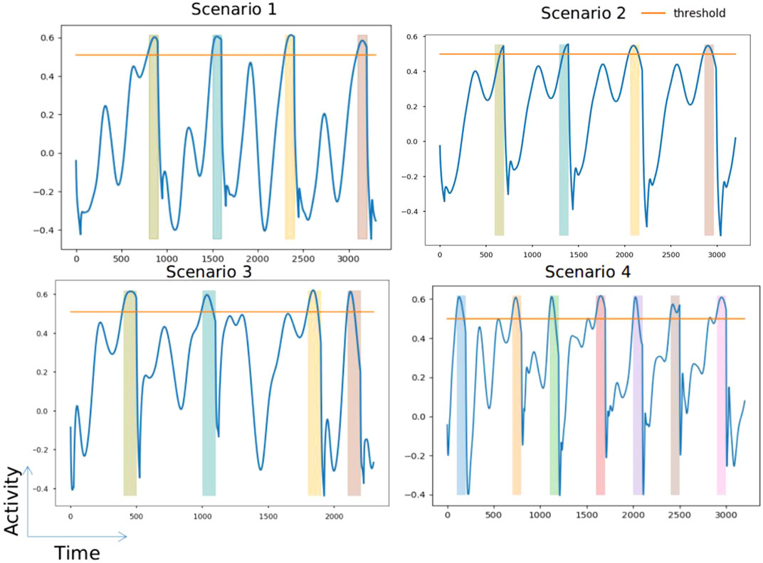
FIGURE 3. Trained activity of four different scenarios. Each scenario contains different times to act. Each colored bar represents the time-to-act interval. The orange line in each figure represents the threshold (=0.5).

The proposed RNN training method exhibited some notable behavioral features, such as the following: 1) the agent learned to subdue its activity as soon as it observed a new state, analogous to restarting a clock, and 2) depending on the observed state, the agent learned to ramp its activity to peak at the time-to-act. We also observed that the agent could learn to do the same without training the recurrent weights (i.e., by only training the output weights $W_{Out}$). However, by training a percentage of the recurrent neurons, we observed that the agent could learn to produce the desired activity in relatively fewer episodes of training.

3.2 Temporal Scaling

It is interesting how humans can execute their actions, such as speaking, writing, or playing music at different speeds. Temporal scaling is another feature we observed in our proposed method. A few studies have explored temporal scaling in humans Diedrichsen et al. (2007); Collier and Wright (1995), particularly the study by Hardy et al. (2018), which modeled temporal scaling using an RNN and a supervised learning method. Their approach involved training recurrent neurons using a second RNN that generates a target output for each of the recurrent neurons in the population. Unfortunately, this approach is not feasible with an online learning algorithm such as reinforcement learning. So, to explore the possibility of temporal scaling with our method, we trained the model using an additional speed input (shown in Figure 4), using the same approach as is outlined in Eqs. 11, 12, 14. In this set-up, the RNN receives both a state input and a speed input. The speed input is a constant value given only when there is a state input; for the rest of the time, the speed input is zero. We trained the model only with one speed ($speed=1$) and tested it at three different speeds: $speed=1.3$, $speed=0.01$, and $speed=0.8$. Figure 5 shows the results. We observed that the shift in click time with respect to $speed$ could be defined using Eq 15. We used a similar procedure to that described in Section 2.3.2 to train for temporal scaling.

$clicktime=clicktime+\left(\left(speed/defaultspeed\right)+200\right)(15)$

FIGURE 4

FIGURE 4. RNN with speed as the input and state input (A) to the RNN (B).

FIGURE 5

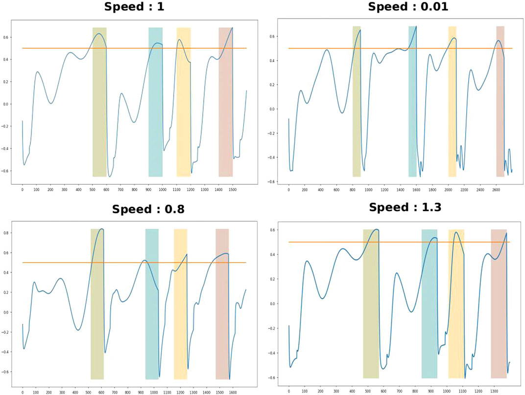
FIGURE 5. RNN activity with a training speed of 1 and test speeds of 0.01, 0.8, and 1.3. The colored bars indicate the expected time-to-act intervals.

3.3 Learning to Plan Multiple Future Times-to-Act

One of the inherent properties of an RNN is that it can produce multiple peaks at different time points, even with only one input at the start of the trial. Results of the study by Hardy et al. (2018) showed that the output of the RNN (trained using supervised learning) peaked at multiple time points given a single input of 250 ms at the start of the trial. To understand whether an agent could learn to plan such multiple future times-to-act given one state using the proposed training, we trained an agent on a slightly modified task-switching scenario. Here, the agent needed to click on the first circle at three different time intervals, 400–500 ms, 1,000–1,100 ms, and 1,700–1,800 ms, and on the second circle at 2,300–2,400 ms. The first circle was set to deactivate at 1,801 ms. At the first state $s1$, the agent learned to produce a neural trajectory that peaked at three intervals, followed by state $s2$, which peaked at 2,300–2,400 ms, as shown in Figure 6.

FIGURE 6

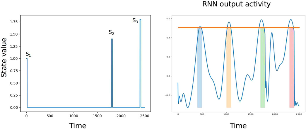
FIGURE 6. Multiple times to act. The state input (A) and output activity (B) which peaks at three different intervals after state $s_1$ and at one interval after state $s_2$. The colored bars indicate the correct time-to-act.

3.4 Skip State Test

As seen in experiment-3, the multiple peaks (multiple times-to-act) that the agent was producing could be based on its inherent property of the RNN. In reinforcement learning, however, the peak at the time-to-act should be truly dependent on each input state and also leverage the temporal properties of the RNN. Hence, to evaluate whether the learned network was truly dependent on the state, we tested it by skipping one of the input states. As Figure 7 shows, when the agent did not receive a state at 2,400 milliseconds, it did not choose to act during the 3,200–3,300 interval, proving that the learned time-to-act is truly state dependent.

FIGURE 7

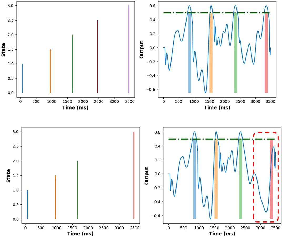
FIGURE 7. Results of the skip state test. The top figures show the state input (left) and the corresponding RNN output (right), where all states are present in the input. The bottom figures show the state input with the fourth skipped state (left), which results in subdued output activity from 3,200 to 3,300 ms (right).

3.5 Task Switching With 20 Tasks

To investigate the scalability of the proposed method to a relatively large state space, we trained and tested the model in a scenario consisting of 20 circles with 20 different times-to-act. Figure 8 demonstrates that the agent could indeed still learn the time-to-act with near-perfect accuracy.

FIGURE 8

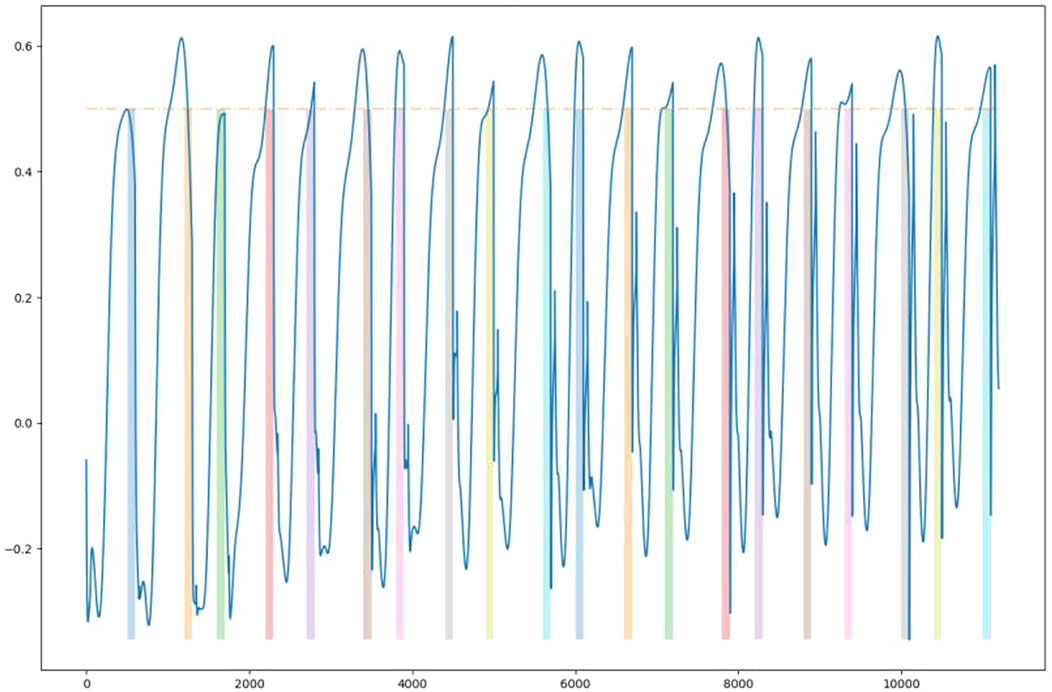
FIGURE 8. RNN output when trained on a scenario with 20 circles. The colored bars indicate the expected time-to-act.

3.6 Memory Task

From the above experiments, the agent was able to learn and employ its time representation in multiple ways. However, we are also interested to know for how long an agent can remember a given input. To investigate this, we delayed the time-to-act for 2,000 ms after the offset of the input and trained the agent. The trained agent remembered a state seen at 0–20 ms until 2,000 ms (see Figure 9), which is indicated by the peak in the output activity. We also trained the agent to remember a state at 3,000 ms. With the current amount of recurrent neurons (i.e., 300 neurons), the agent was not able to remember for 3,000 ms from the offset of an input.

FIGURE 9

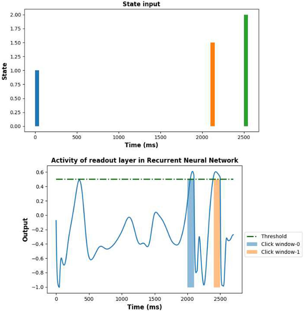
FIGURE 9. RNN output when trained on a scenario with two circles, where the first circle must be clicked after 2,000 ms. The colored bars indicate the expected time-to-act.

3.7 Shooting a Moving Target

Similar to the task-switching experiment, we trained the RL agent to learn “when to act” on a different scenario. In this scenario, the agent is rewarded for shooting a moving target. The target is the blob of a moving damped pendulum. The length of the pendulum is 1 m, and the weight of the blob is 1 kg. We trained the DQN to select the direction of shooting and the RNN to learn the exact time to release the trigger. The agent was rewarded positively for hitting the blob with an error of 0.1 m and negatively if the agent missed the target. The learned activity is shown in Figure 10; the left shows the motion of the pendulum and the right shows the learned RNN activity. The threshold in this experiment was 0.05, and the agent was able to hit the blob 5 times in 3,000 ms. Although it is still not clear why the agent did not peak its activity from 0 to 1,500 ms, the agent showed better performance after 1,500 ms.

FIGURE 10

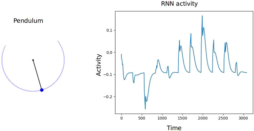
FIGURE 10. Left shows the pendulum scenario. The pendulum rod (the black line) is 1 m long, and the blob (blue dot) weighs 1 kg. Right shows the training RNN activity.

4 Comparison With Long Short-Term Memory (LSTM) Network

A recent study by Deverett et al. (2019) investigated the interval timing abilities in a reinforcement learning agent. In the study, an RL agent was trained to reproduce a given temporal interval. However, the time representation in the study was in the form of movement (or velocity) control. In other words, the agent had to move from one point to the goal point within the same interval as presented at the start of the experiment. The agent which used the LSTM network in this study by Deverett et al. (2019) performed the task with near-perfect accuracy, indicating the ability to learn temporal properties using LSTM networks. Following these findings, our study endeavors to understand if an agent can learn a direct representation of time (instead of an indirect representation of time, such as velocity or acceleration) using LSTM.

In order to investigate in this direction, we trained an RL agent with only one LSTM network as its DQN network (no RNN was used in this test) on the same task-switching scenario. The input sequence for an RNN works in terms of $dt$ (as shown in Eq 6), whereas input for LSTM works in terms of sequence length, as shown in Figure 11. For example, an input signal with a length of 3,000 ms can be given as 1 ms at a time to an RNN, and for LSTM, the same input should be divided into a fixed length to effectively capture the temporal properties in the input. We used an LSTM with 100 input nodes and gave an input signal of 100 ms to the network, followed by the next 100 ms. Indeed, the sequence length can be smaller than 100 ms. In our experiments, we trained the agent with different sequence lengths (50, 100, 200, and 300 ms), and the agent showed better performance for 300 ms (results for 50, 100, and 200 ms are given in the Appendix). The architecture of the LSTM we used contained one LSTM layer with 256 hidden units, 300 input nodes, and two linear layers with 100 nodes each. The output size of the network was 300, which resulted in an activity of n points for a given input signal of $nms$. The hidden states of the LSTM network were carried on throughout the episode.

FIGURE 11

FIGURE 11. Input difference between the RNN and the LSTM network.

The trained activity of the LSTM network is shown in Figure 12 (bottom), where the light blue region shows the output activity of the network. The colored bars in Figure 12 show the output activity of the LSTM network and the correct time-to-act intervals for clicking each circle. The LSTM network did learn to exceed the threshold indicating when to act at a few time-to-act intervals. However, there is periodicity learned by the network, meaning that for every 300 ms, the network learned to produce similar activity.

FIGURE 12

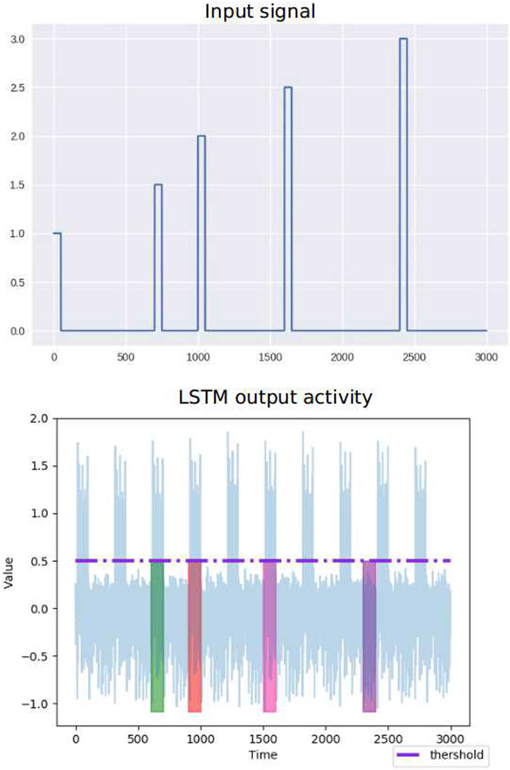
FIGURE 12. Output activity of the trained LSTM network for a task-switching scenario containing four circles, with time-to-act intervals shown in colored bars.

5 Discussion

In this study, we trained a reinforcement learning agent to learn “when to act” using an RNN and “what to act” using a DQN. We introduced a reward-based recursive least square algorithm to train the RNN. By disentangling the process of learning the temporal and spatial aspects of action into independent tasks, we intend to understand explicit time representation in an RL agent. Through this strategy, the agent learned to create its representation of time. Our experiments, which employed a peak-interval style, show that the agent could learn to produce a neural trajectory that peaked at the time-to-act with near-perfect accuracy. We also observed several other intriguing behaviors.

• The agent learned to subdue its activity immediately after observing a new state. We interpreted this as the agent restarting its clock.

• The agent was able to temporally scale its actions in our proposed learning method. Even though we trained the agent with a single-speed value ($speed=1$), it learned to temporally scale its action to speeds that were both lower ($speed=0.01$) and higher ($speed=1.3$) than the trained speed. Notably, the agent was not able to scale its actions beyond $speed=1.3$.

• We observed that neural networks such as the LSTM might not be able to learn an explicit representation of time when compared with population clock models. Deverett et al. (2019) showed that an RL agent can scale its actions (increase or decrease the velocity) using the LSTM network. However, when we trained the LSTM network to learn a direct representation of the time, it learned periodic activity.

• In this research study, we trained an RL agent in a similar environment to task switching; shooting a moving target. The target in our experiment is a blob of a damped pendulum with a length of 1 m and a mass of 1 kg. The agent was able to shoot the fast-moving blob by learning to shoot at a few near-accurate time points.

Data Availability Statement

The raw data supporting the conclusions of this article will be made available by the authors, without undue reservation.

Author Contributions

All authors listed have made a substantial, direct, and intellectual contribution to the work and approved it for publication.

Conflict of Interest

The authors declare that the research was conducted in the absence of any commercial or financial relationships that could be construed as a potential conflict of interest.

Publisher’s Note

All claims expressed in this article are solely those of the authors and do not necessarily represent those of their affiliated organizations, or those of the publisher, the editors and the reviewers. Any product that may be evaluated in this article, or claim that may be made by its manufacturer, is not guaranteed or endorsed by the publisher.

Acknowledgments

This work was supported in part by the Australian Research Council (ARC) under discovery grant DP180100656 and DP210101093. Research was also sponsored in part by the Australia Defence Innovation Hub under Contract No. P18-650825, US Office of Naval Research Global under Cooperative Agreement Number ONRG ‐ NICOP ‐ N62909‐19‐1‐2058, and AFOSR ‒ DST Australian Autonomy Initiative agreement ID10134. We also thank the NSW Defence Innovation Network and NSW State Government of Australia for financial support in part of this research through grant DINPP2019 S1‐03/09 and PP21‐22.03.02.

References

Åström, K. J., and Wittenmark, B. (2013). Computer-controlled Systems: Theory and Design. Englewood Cliffs, NJ: Courier Corporation.

Bakker, B. (2002). “Reinforcement Learning with Long Short-Term Memory,” in Proceedings of the 14th International Conference on Neural Information Processing Systems: Natural and Synthetic, Vancouver, Canada, 1475–1482.

Google Scholar

Buonomano, D. V., and Laje, R. (2011). “Population Clocks,” in Space, Time And Number In the Brain (Elsevier), 71–85. doi:10.1016/b978-0-12-385948-8.00006-2

CrossRef Full Text | Google Scholar

Buonomano, D. V., and Maass, W. (2009). State-dependent Computations: Spatiotemporal Processing in Cortical Networks. Nat. Rev. Neurosci. 10, 113–125. doi:10.1038/nrn2558

PubMed Abstract | CrossRef Full Text | Google Scholar

Carrara, N., Leurent, E., Laroche, R., Urvoy, T., Maillard, O. A., and Pietquin, O. (2019). “Budgeted Reinforcement Learning in Continuous State Space,” in Advances in Neural Information Processing Systems 32: Annual Conference on Neural Information Processing Systems 2019, NeurIPS 2019, Vancouver, BC, December 8–14, 2019, 9295–9305.

Google Scholar

Chung, J., Gulcehre, C., Cho, K., and Bengio, Y. (2014). Empirical Evaluation of Gated Recurrent Neural Networks on Sequence Modeling in NIPS 2014 Workshop on Deep Learning, Quebec, Canada, December, 2014. preprint arXiv:1412.3555.

Collier, G. L., and Wright, C. E. (1995). Temporal Rescaling of Simple and Complex Ratios in Rhythmic Tapping. J. Exp. Psychol. Hum. Perception Perform. 21, 602–627. doi:10.1037/0096-1523.21.3.602

PubMed Abstract | CrossRef Full Text | Google Scholar

Deverett, B., Faulkner, R., Fortunato, M., Wayne, G., and Leibo, J. Z. (2019). “Interval Timing in Deep Reinforcement Learning Agents,” in 33rd Conference on Neural Information Processing Systems (NeurIPS 2019), Vancouver, Canada, 6689–6698.

Google Scholar

Diedrichsen, J., Criscimagna-Hemminger, S. E., and Shadmehr, R. (2007). Dissociating Timing and Coordination as Functions of the Cerebellum. J. Neurosci. 27, 6291–6301. doi:10.1523/jneurosci.0061-07.2007

PubMed Abstract | CrossRef Full Text | Google Scholar

Doya, K. (2000). Reinforcement Learning in Continuous Time and Space. Neural Comput. 12, 219–245. doi:10.1162/089976600300015961

PubMed Abstract | CrossRef Full Text | Google Scholar

Durstewitz, D. (2003). Self-organizing Neural Integrator Predicts Interval Times through Climbing Activity. J. Neurosci. 23, 5342–5353. doi:10.1523/jneurosci.23-12-05342.2003

PubMed Abstract | CrossRef Full Text | Google Scholar

Hardy, N. F., Goudar, V., Romero-Sosa, J. L., and Buonomano, D. V. (2018). A Model of Temporal Scaling Correctly Predicts that Motor Timing Improves with Speed. Nat. Commun. 9, 4732–4814. doi:10.1038/s41467-018-07161-6

PubMed Abstract | CrossRef Full Text | Google Scholar

Hochreiter, S., and Schmidhuber, J. (1997). Long Short-Term Memory. Neural Comput. 9, 1735–1780. doi:10.1162/neco.1997.9.8.1735

PubMed Abstract | CrossRef Full Text | Google Scholar

Klapproth, F. (2008). Time and Decision Making in Humans. Cogn. Affective, Behav. Neurosci. 8, 509–524. doi:10.3758/cabn.8.4.509

PubMed Abstract | CrossRef Full Text | Google Scholar

Laje, R., and Buonomano, D. V. (2013). Robust Timing and Motor Patterns by Taming Chaos in Recurrent Neural Networks. Nat. Neurosci. 16, 925–933. doi:10.1038/nn.3405

PubMed Abstract | CrossRef Full Text | Google Scholar

Li, D., Ge, S. S., He, W., Ma, G., and Xie, L. (2019). Multilayer Formation Control of Multi-Agent Systems. Automatica 109, 108558. doi:10.1016/j.automatica.2019.108558

CrossRef Full Text | Google Scholar

Lillicrap, T. P., Hunt, J. J., Pritzel, A., Heess, N., Erez, T., Tassa, Y., et al. (2015). Continuous Control with Deep Reinforcement Learning. 4th International Conference on Learning Representations, (ICLR), San Juan, Puerto Rico, May 2–4, 2016. preprint arXiv:1509.02971.

Matell, M. S., Meck, W. H., and Nicolelis, M. A. L. (2003). Interval Timing and the Encoding of Signal Duration by Ensembles of Cortical and Striatal Neurons. Behav. Neurosci. 117, 760–773. doi:10.1037/0735-7044.117.4.760

PubMed Abstract | CrossRef Full Text | Google Scholar

Miall, C. (1989). The Storage of Time Intervals Using Oscillating Neurons. Neural Comput. 1, 359–371. doi:10.1162/neco.1989.1.3.359

CrossRef Full Text | Google Scholar

Mnih, V., Kavukcuoglu, K., Silver, D., Graves, A., Antonoglou, I., Wierstra, D., et al. (2013). Playing Atari with Deep Reinforcement Learning. arXiv. preprint arXiv:1312.5602.

Mnih, V., Kavukcuoglu, K., Silver, D., Rusu, A. A., Veness, J., Bellemare, M. G., et al. (2015). Human-level Control through Deep Reinforcement Learning. Nature 518, 529–533. doi:10.1038/nature14236

PubMed Abstract | CrossRef Full Text | Google Scholar

Oh, K.-K., Park, M.-C., and Ahn, H.-S. (2015). A Survey of Multi-Agent Formation Control. Automatica 53, 424–440. doi:10.1016/j.automatica.2014.10.022

CrossRef Full Text | Google Scholar

Petter, E. A., Gershman, S. J., and Meck, W. H. (2018). Integrating Models of Interval Timing and Reinforcement Learning. Trends. Cogn. Sci. 22, 911–922. doi:10.1016/j.tics.2018.08.004

PubMed Abstract | CrossRef Full Text | Google Scholar

Silver, D., Schrittwieser, J., Simonyan, K., Antonoglou, I., Huang, A., Guez, A., et al. (2017). Mastering the Game of Go without Human Knowledge. Nature 550, 354. doi:10.1038/nature24270

PubMed Abstract | CrossRef Full Text | Google Scholar

Simen, P., Balci, F., deSouza, L., Cohen, J. D., and Holmes, P. (2011). A Model of Interval Timing by Neural Integration. J. Neurosci. 31, 9238–9253. doi:10.1523/jneurosci.3121-10.2011

PubMed Abstract | CrossRef Full Text | Google Scholar

Sompolinsky, H., Crisanti, A., and Sommers, H.-J. (1988). Chaos in Random Neural Networks. Phys. Rev. Lett. 61, 259. doi:10.1103/physrevlett.61.259

PubMed Abstract | CrossRef Full Text | Google Scholar

Tallec, C., Blier, L., and Ollivier, Y. (2019). Making Deep Q-Learning Methods Robust to Time Discretization. International conference on machine learning (ICML), Long Beach. arXiv. preprint arXiv:1901.09732.

Vinyals, O., Babuschkin, I., Czarnecki, W. M, Mathieu, M., Dudzik, A., Junyoung, C., et al. (2019). Grandmaster level in StarCraft II using multi-agent reinforcement learning. Nature 575, 350–354.

Google Scholar

Watkins, C. J., and Dayan, P. (1992). Q-learning. Machine Learn. 8, 279–292. doi:10.1023/a:1022676722315

CrossRef Full Text | Google Scholar

Xue, D., Yao, J., Wang, J., Guo, Y., and Han, X. (2013). Formation Control of Multi-Agent Systems with Stochastic Switching Topology and Time-Varying Communication Delays. IET Control. Theor. Appl. 7, 1689–1698. doi:10.1049/iet-cta.2011.0325

CrossRef Full Text | Google Scholar