
95% of researchers rate our articles as excellent or good
Learn more about the work of our research integrity team to safeguard the quality of each article we publish.
Find out more
ORIGINAL RESEARCH article
Front. Comput. Neurosci. , 23 February 2024
Volume 18 - 2024 | https://doi.org/10.3389/fncom.2024.1347748
This article is part of the Research Topic Women in Computational Neuroscience View all articles
 Gurpreet Jagdev1
 Na Yu1,2*
Synchronous dynamics play a pivotal role in various cognitive processes. Previous studies extensively investigate noise-induced synchrony in coupled neural oscillators, with a focus on scenarios featuring uniform noise and equal coupling strengths between neurons. However, real-world or experimental settings frequently exhibit heterogeneity, including deviations from uniformity in coupling and noise patterns. This study investigates noise-induced synchrony in a pair of coupled excitable neurons operating in a heterogeneous environment, where both noise intensity and coupling strength can vary independently. Each neuron is an excitable oscillator, represented by the normal form of Hopf bifurcation (HB). In the absence of stimulus, these neurons remain quiescent but can be triggered by perturbations, such as noise. Typically, noise and coupling exert opposing influences on neural dynamics, with noise diminishing coherence and coupling promoting synchrony. Our results illustrate the ability of asymmetric noise to induce synchronization in such coupled neural oscillators, with synchronization becoming increasingly pronounced as the system approaches the excitation threshold (i.e., HB). Additionally, we find that uneven coupling strengths and noise asymmetries are factors that can promote in-phase synchrony. Notably, we identify an optimal synchronization state when the absolute difference in coupling strengths is maximized, regardless of the specific coupling strengths chosen. Furthermore, we establish a robust relationship between coupling asymmetry and the noise intensity required to maximize synchronization. Specifically, when one oscillator (receiver neuron) receives a strong input from the other oscillator (source neuron) and the source neuron receives significantly weaker or no input from the receiver neuron, synchrony is maximized when the noise applied to the receiver neuron is much weaker than that applied to the source neuron. These findings reveal the significant connection between uneven coupling and asymmetric noise in coupled neuronal oscillators, shedding light on the enhanced propensity for in-phase synchronization in two-neuron motifs with one-way connections compared to those with two-way connections. This research contributes to a deeper understanding of the functional roles of network motifs that may serve within neuronal dynamics.
The synchronization of neural oscillations is acknowledged for its role in facilitating communication between neurons (Varela et al., 2001; Fell and Axmacher, 2011), and is essential for higher order cognitive processes including memory formation, motor coordination, and sensory information processing (Varela et al., 2001; Womelsdorf and Fries, 2007; Kawasaki et al., 2018). Noise, prevalent in real neural networks, plays a crucial role in giving rise to emergent dynamics that may serve important physiological functions (Varela et al., 2001; Fell and Axmacher, 2011). One intriguing constructive effect of noise is noise-induced synchrony, wherein noise alone can induce coordinated and synchronized dynamics. This phenomenon has been widely explored, especially in neural networks, as shown by studies such as (Perc and Marhl, 2006; Perc, 2007; Touboul et al., 2020). Network motifs are frequently recurring structural patterns in neuronal networks, commonly regarded as the fundamental building blocks of complex networks (Milo et al., 2002; Reigl et al., 2004). Among network motifs, those featuring two neurons are notably more prevalent than other multi-neuron motifs (Reigl et al., 2004; Song et al., 2005), making them central to shaping the collective behavior of the network. Consequently, this study focuses on the noise-induced synchrony of the most over-represented motifs: two-neuron motifs.
In the context of two-neuron motifs or two coupled oscillators, prior research has extensively studied the noise-induced synchrony under homogeneous configurations such as common noise (where each neuron encounters identical noise), symmetric noise where each neuron has independent noise but with equal noise intensity), and couplings of exactly equal strengths between neurons. These investigations are well-documented in reviews and books (Rosenblum et al., 2001; Pikovsky, 2002; Boccaletti et al., 2006). In real-world or experimental scenarios, however, coupling and noise patterns often deviate from uniformity (Song et al., 2005; Morgan and Soltesz, 2008). Our understanding of the broader implications associated with the effects of asymmetric noise (where each neuron receives independent noise sources with different noise intensities) and uneven coupling (e.g., unequal coupling strength) is limited, as only a few studies have explored the influence of heterogeneity in noise and/or coupling on the dynamics of two coupled neuronal oscillators. For example, the interplay between uneven coupling strengths and symmetric noise in two coupled oscillators has been shown to promote synchronization (Blasius, 2005) and enhance the transmission of sub-threshold external signals (Masoliver and Masoller, 2018). In a pair of coupled oscillators with uneven coupling and asymmetric additive noise (Amro et al., 2015) finds that the phase coherence of one oscillator is a non-monotonic function of the additive noise applied to the other oscillator: as the phase coherence of one oscillator decreases, the other increases.
To address these less explored aspects, this paper investigates the synchronous dynamics of a pair of excitable neurons in the presence of two sources of heterogeneity: asymmetric noise and uneven coupling. Here the excitable neurons are modeled by the normal form of a Hopf bifurcation (HB), a deterministic framework underpinning critical transitions between quiescent and oscillatory states in complex systems. Therefore our findings provide a versatile framework for illustrating a diverse array of dynamical patterns near a HB within a heterogeneous configuration. Given that the two-neuron motif constitutes a fundamental element in a neuronal network, this study contributes valuable insights into the generation of diverse network behaviors in the context of heterogeneity in both noise and coupling. The structure of the remainder of this paper is as follows: Section 2 provides an introduction to the mathematical model and the methodologies used. In Section 3.1, we present the bifurcation diagram of two deterministic oscillators and Section 3.2 introduces noise-induced oscillations. Section 3.3 focuses on demonstrating noise-induced synchrony and how asymmetric noise affects this synchrony. In Section 3.4, we study the effects of the bifurcation parameter on synchronization, and in Section 3.5, we examine the dual effects of uneven coupling and asymmetric noise on synchrony. Finally, Section 4 offers a summary and engages in a discussion of the findings.
Synchrony in neural oscillators is not solely determined by their phase; rather, the statistical prevalence of amplitude dynamics influencing synchronization is noteworthy (Gambuzza et al., 2016). This phenomenon, referred to as amplitude-sensitive synchrony, is a distinctive characteristic of oscillators located near an HB. Hence, our research employs the λ−ω system, recognized as a minimal model (or normal form), capable of capturing both amplitude and phase dynamics of an oscillator in the proximity of a HB. Therefore, the insights gained from this study have broader applicability to other dynamical systems situated in the vicinity of a HB.
We examine a duo of coupled λ−ω oscillators, selected with specific parameters that position the model near a supercritical HB. In the absence of noise, these oscillators remain quiescent, but they become excited upon the introduction of an intrinsic noise stimulus. Their coupling strength is uneven, and they are subjected to asymmetric intensities of additive noise. Moreover, both oscillators are represented by the set of stochastic differential equations (SDEs).
where i, j = 1, 2. represents the amplitude of the ith oscillator. controls the increment and decrement of the amplitude of the ith oscillator. λ0 is the control parameter and a HB occurs at λ0 = 0 (see Figure 1A). determines the increment and decrement of the frequency of the ith oscillator. We consider a supercritical HB by setting the parameter values as α = −0.2, γ = −0.2, ω0 = 2, and ω1 = 0. di(xj − xi) and di(yj − yi) represent diffusive coupling between oscillators i and j with oscillator specific coupling strength, di, i = 1, 2. δidηi(t) represents an independent intrinsic noise applied to xi (i.e., the noise is unique to each oscillator) where ηi(t) is a Wiener process with zero mean and unity variance and δi is the noise intensity. We restrict our attention to the excitatory coupling in the range 0.01 ≤ d1, d2 ≤ 0.3 (as in Yu et al., 2008).
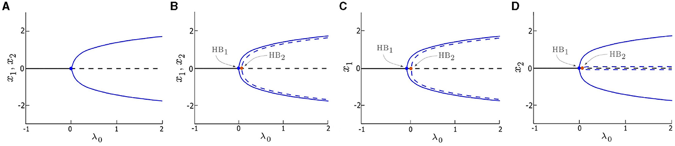
Figure 1. Bifurcation diagrams of the deterministic system (δ1 = δ2 = 0) vs. control parameter λ0. (A) single/uncoupled oscillator (x = x1 = x2) with d1 = d2 = 0, a single Hopf bifurcation (HB) occurs at λ = 0. (B) symmetrically coupled oscillators (x1, x2) with d1 = d2 = 0.05, (C, D) asymmetrically coupled oscillators (x1 and x2, respectively) with d1 = 0.1 and d2 = 0.01. Two HB points, HB1 and HB2, occur and are indicated by blue and orange dots, respectively. The value of λ0 corresponding to HB1 is zero in (B–D). Stable solutions are marked by solid blue lines and solid black lines, and unstable solutions are marked by dashed blue lines and dashed black lines. Other parameters are: α = −0.2; γ = −0.2; ω0 = 2; and ω1 = 0.
To study the interplay of noise and coupling and its effect on the synchronization of our model we analyze the synchrony of both oscillators when subject to the additive noise, δidηi, i = 1, 2. Since the oscillators rotate about the fixed point (xi, yi) = (0, 0), i = 1, 2, when driven by noise, the time-dependent phase of each oscillator is taken to be the natural phase (Rosenblum et al., 2001),
i = 1, 2. In the classical treatment of phase analysis, synchrony measures are often based on the distribution of the phase difference, Δϕn,m = nϕ2 − mϕ1, where n, m ∈ ℕ characterize the order of locking (Rosenblum et al., 2001, 2022). However, in the presence of noise, the phase of the oscillators can exhibit random jumps of ±2π, called phase slips, which can cause the phase difference, Δϕn,m, to compound errors, and lead to erroneous results. Therefore, instead of considering the natural phase in Equation 4, we consider the cyclic relative phase (Mormann et al., 2000; Rosenblum et al., 2001),
which is the natural phase wrapped over the unit circle. This procedure ensures that errors in Δφn,m caused by phase slips do not compound which leads to more stable numerical results. Furthermore, for simplicity, we consider only 1 − 1 synchronization: Δφ = Δφ1,1.
The bifurcation diagrams (i.e., Figures 1, 2) are generated using XPPAUT software (Ermentrout, 2012). All further analysis (i.e., Figures 3–9) is conducted using MATLAB. To simulate the SDEs in Equations 1, 2 we use the Euler-Maruyama method with time-step dt = 0.01 and arbitrary random initial conditions , i = 1, 2. Due to the nature of white noise, noise-induced oscillations contain high-frequency fluctuations at very low or very high noise intensities, which poses difficulties in the computation of phase. Hence, to achieve more consistent numerical results a low-pass filter is applied to remove high-frequency fluctuations. The signal-to-noise ratio, β, and synchronization measures |Δφ|, R, and ρ in Equations 6–9, respectively, are averaged over N = 200 trials. The XPPAUT and MATLAB source code can be found at: https://github.com/TMUcode/CoupleNeurons.
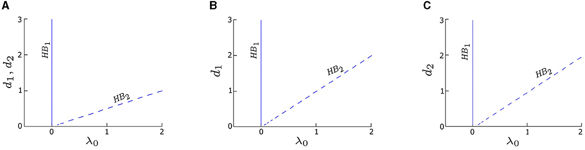
Figure 2. Two-parameter bifurcation diagrams (coupling strength di vs. λ0) for three coupling cases: (A) symmetric coupling strengths, d1 = d2, (B) asymmetric coupling strengths with varying d1 and fixed d2 = 0.05, and (C) asymmetric coupling strengths with varying d2 and fixed d1 = 0.05. The branches labeled HB1 (solid blue) and HB2 (dashed blue) represent the same two distinct HB points in Figure 1. The value of λ0 corresponding to HB1 is consistently zero across three cases, aligning with the observation in Figure 1. Conversely, the value of λ0 corresponding to HB2 linearly increases with di. Other parameters are: δ1 = δ2 = 0; α = −0.2; γ = −0.2; ω0 = 2; and ω1 = 0.
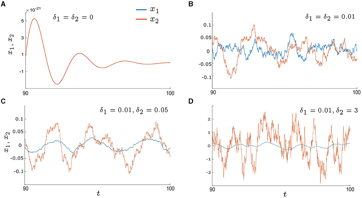
Figure 3. Time series of x1andx2 in the excitable regime (λ0 < 0) with various noise intensities: (A) δ1 = δ2 = 0, (B) δ1 = δ2 = 0.01, (C) δ1 = 0.01 and δ2 = 0.05, and (D) δ1 = 0.01 and δ2 = 3. The blue lines represent x1 and the orange lines represent x2. (A) shows the deterministic system with a stable fixed point at xi = 0, resulting in an overlap between x1 and x2. (B–D) illustrate the noise-induced oscillations, with (C) showing higher levels of regularity and synchrony in comparison to (B, D). Other parameters are: α = −0.2; γ = −0.2; ω0 = 2; ω1 = 0; λ0 = −0.5; d1 = 0.3; and d2 = 0.01.
The dynamics of the deterministic system (δ1 = δ2 = 0) are examined in this section. We consider three cases and compare their bifurcation diagrams: single (i.e., uncoupled) oscillators with d1 = d2 = 0 (Figure 1A), two symmetrically coupled oscillators with d1 = d2 ≠ 0 (Figure 1B), and two asymmetrically coupled oscillators with d1 ≠ d2 (Figures 1C, D). When λ0 < 0, both oscillators in all three cases are quiescent, they rest at stable fixed points, as shown in Figure 1 (solid black line). Conversely, when λ0 > 0, the fixed points are destabilized (dashed black line), and stable periodic orbits emerge (solid blue line) in all three cases. Both isolated (Figure 1A) and coupled (Figures 1B–D) oscillators undergo a supercritical HB (denoted as HB1) at λ0 = 0. However, when the oscillators are coupled, the system exhibits a second HB (denoted as HB2) which leads to unstable periodic orbits (dashed blue line in Figures 1B–D).
When the oscillators are symmetrically coupled (e.g., d1, d2 = 0.05 in Figure 1B), the amplitudes of the periodic orbits generated by both oscillators are identical for each λ0 value, however, the unstable periodic orbits have an amplitude that is slightly less than the amplitude of the stable periodic orbits. When the oscillators are coupled asymmetrically (e.g., d1 = 0.1 and d2 = 0.01 in Figures 1C, D), the bifurcation diagram for one oscillator (Figure 1C) is identical to its counterpart in Figure 1B, whereas, the bifurcation diagram of the other oscillator (Figure 1D) shows a single difference: the amplitude of the unstable periodic orbit is near zero, which is much smaller counterpart in Figure 1B.
To further explore the effects of coupling on the deterministic system, we calculate the two-parameter bifurcation diagrams of our model by taking both the coupling strength, di, and λ0 as control parameters. The trajectory of HB1 (solid blue line) in the two-parameter bifurcation diagram in Figure 2 indicates the transition of the system between the quiescent and oscillatory states in the deterministic regime remains the same (λ0 = 0) no matter the coupling strength. Moreover, the deterministic system is quiescent when λ0 < 0, but can be excited by an external stimulus (e.g., noise) to produce oscillations. Thus, we refer to the left side of HB1 as the excitable regime, and the right side of HB1 as the oscillatory regime.
Although HB2 is not a determinant factor of the excitability in the deterministic regime, we find that it has a relationship with the coupling strength: λ0 ≈ d1 + d2. Specifically, when the coupling is symmetric (d1 = d2), HB2 occurs at λ0 ≈ 2di, i = 1or2, resulting in a line with a slope approximately equal to 1/2, as depicted by the dashed blue line in Figure 2A. For asymmetric couplings, such those obtained by varying d1 while fixing d2 = 0.05, HB2 appears as a straight line with a slope approximately equal to 1 (dashed blue line in Figure 2B), since λ0 ≈ d1 + 0.05. Another example of asymmetric coupling is obtained by varying d2 while fixing d1 = 0.05, which yields a straight line with the equation λ0 ≈ d2 + 0.05 (dashed blue line in Figure 2C).
In this section, we study noise-induced oscillations. The control parameter λ0 is set to be in the excitable regime, for example, λ0 = −0.5. As a result, the deterministic system, with δ1 = δ2 = 0, displays damped oscillations that eventually converge to the fixed point (xi = yi = 0, i = 1, 2), as illustrated in Figure 3A. However, when the intrinsic noise, δidηi, is introduced, it can trigger repeated excursions from the stable fixed point which leads to oscillatory motion; otherwise known as noise-induced oscillations. Examples are presented in Figures 3B–D which display sample time series of x1 and x2 in the presence of the intrinsic noise stimulus with different intensities. When the noise intensity is small and symmetric (e.g. δ1 = δ2 = 0.01 in Figure 3B) there are intermittent periods of phase drift and phase locking; both in-phase and anti-phase. When the noise intensities become asymmetric by increasing one of the noise intensities, for example, δ1 = 0.01 and δ2 = 0.05 as in Figure 3C, the time series for x1 (blue line) and x2 (orange line) exhibit increased regularity and longer epochs of in-phase locking. Furthermore, if δ2 is increased further, for example, δ2 = 3 as in Figure 3D, the oscillations of x2 become less regular and more chaotic. Overall, these examples demonstrate that synchrony can be optimized by tuning just one of the noise intensities to be an intermediate value.
To determine an appropriate range of noise intensities, δ1 and δ2, we make use of the signal-to-noise ratio measure (Gang et al., 1993; Pikovsky and Kurths, 1997).
where hp and ωp denote the height and central frequency of the power spectrum density peak of x, respectively, and Δω denotes the width of the power spectrum density peak at half-maximal power, . We have computed the relationship between β and δ for a single λ−ω oscillator, (x, y), and present the results in Figure 4. When δ < 0.01, we find β is significantly small, indicating that the noise level is too weak. However, as the level of noise gradually increases, the β curve displays a peak around δ = 0.9, indicating that this noise intensity is optimal. For larger values of δ, specifically, when δ > 0.9, we observe a sharp decrease in β, suggesting that the noise intensity is now overpowering the regularity of oscillations. Therefore, based on these observations, we select the range 0.01 ≤ δ1, δ2 ≤ 5 for our analysis.
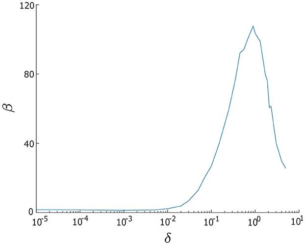
Figure 4. Signal-to-noise ratio measure β vs. noise intensity δ for a single/uncoupled neuron oscillator in the excitable regime (λ0 < 0). Greater regularity in noise-induced oscillations is indicated by larger values of β. The largest β occurs when noise intensity is δ = 0.9. Other parameters are: α = −0.2; γ = −0.2; ω0 = 2; ω1 = 0; and λ0 = −0.5.
The results presented in Section 3.2 suggest that the synchrony of our system with asymmetric noise and uneven coupling can be optimized by adjusting the noise intensities, δ1 and δ2. To quantify the effects of noise on the synchrony of our model more rigorously, we introduce three measures of synchrony. The first measure is the absolute phase difference, denoted |Δφ|, which is defined as
where φi(t) is the phase of the ith oscillator. Since our model considers excitatory coupling, we focus on the in-phase dynamics of the oscillators, such that smaller values of |Δφ| correspond to a greater degree of synchrony. The second measure we use is the mean phase coherence, denoted R, which is defined as (Mormann et al., 2000; Rosenblum et al., 2001),
where Δφ = φ1 − φ2. The value of R ranges from 0 to 1, and larger values of R indicate a greater degree of synchrony. The third synchronization measure we use is the normalized synchronization index, denoted ρ, which is defined as (Rosenblum et al., 2001),
where is the Shannon entropy, Smax = lnM is the maximum entropy, pk refers to the probability of finding Δφ in the kth bin of the histogram, and M is the total number of bins. The quantity ρ is normalized to 0 ≤ ρ ≤ 1, and smaller values of ρ indicate a narrower distribution of Δφ and thus a greater degree of synchrony.
To begin we consider the effect of a single noise intensity on the degree of synchrony between two unevenly coupled oscillators. To achieve this, we set d1 ≠ d2, fix one noise intensity to be δ1 = 0.05, and vary the other noise intensity, δ2, from 0.01 to 5 and compute the level of synchrony using the three measures listed above. We present the results in Figure 5A, where the blue, orange, and black curves correspond to |Δφ|, R, and ρ, respectively. For weak δ2, both ρ and |Δφ| show a rapid decrease while R displays a rapid increase. These consistent results suggest that the level of synchrony is increasing. However, for strong δ2, we notice an opposite trend, where ρ and |Δφ| increase while R decreases, indicating a decrease in the level of synchrony.
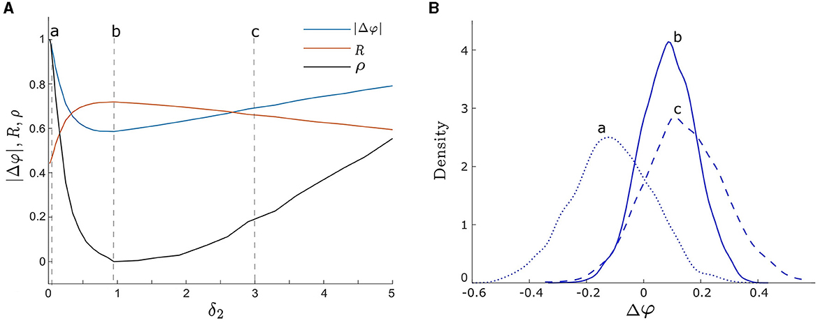
Figure 5. (A) Three measures of phase synchronization: |Δφ| (the absolute value of the phase difference), R (the mean phase coherence), and ρ (the synchronization index) vs. δ2. The orange, blue, and black curves correspond to R, |Δφ|, and ρ, respectively. The three vertical dashed lines labeled by a, b, and c correspond to δ2 = 0.05, 0.95, and3, respectively. Smaller values of |Δφ| and ρ, and larger values of R indicate greater noise-induced synchrony. All three measures demonstrate consistent synchrony dynamics as δ2 varies, reaching maximum synchrony at δ2 = 0.95. (B) The empirical probability density functions of Δφ, with the curves a, b, and c corresponding to noise intensities δ2 = 0.05, 0.95, and 3 as in (A), respectively. The peaks of density functions corresponding to a, b, and c are Δφ = −0.12, 0.08, and 0.12, respectively. Curve b with δ2 = 0.95 exhibits the most concentrated distribution of Δφ, indicating optimal noise-induced synchrony, consistent with the finding in (A). Other parameters are: δ1 = 0.05; α = −0.2; γ = −0.2; ω0 = 2; ω1 = 0; λ0 = −0.5; d2 = 0.01; and d1 = 0.3.
Furthermore, synchrony is maximized at an intermediate noise intensity, which we find to be δ2 = 0.95 for all three measures in Figure 5A. Notice that it is close to the optimal noise intensity of a single oscillator as shown in Figure 4. These changes in synchrony may also be observed from the probability density functions of Δφ shown in Figure 5B. The dotted blue curve (labeled a), solid blue curve (labeled b), and dashed blue curve (labeled c) correspond to noise intensities δ2 = 0.05, 0.95, and3, respectively (i.e., points a, b, and c in Figure 5A). As δ2 increases from weak to intermediate levels, the center of the distribution of Δφ shifts from small negative values toward the point Δφ = 0, which represents in-phase synchronization. Moreover, the distribution of Δφ is centered at 0.08 at the optimal noise intensity δ2 = 0.95 in Figure 5A. Additionally, the width and peak of the distribution become narrower and higher, respectively, indicating a more concentrated distribution of phase differences between the two oscillators (i.e., a higher level of synchrony). As the noise intensity continues to increase, the center of the Δφ distribution remains almost unchanged, but its width and peak increase and decrease, respectively, which is indicative of a lower degree of synchrony.
Next, we investigate how both noise intensities, δ1 and δ2, affect the level of synchrony between two unevenly coupled oscillators. To systematically examine their influence, we generate heat maps, which represent the level of synchrony using the measures |Δφ| and R over the parameter space 0.01 ≤ δ1, δ2 ≤ 5, as illustrated in Figures 6A, B, respectively. In Figure 6A, warmer colors indicate larger values of |Δφ| (i.e., lower levels of synchrony), while cooler colors correspond to smaller values of |Δφ| (i.e., higher levels of synchrony). Note, a three-dimensional representation of Figure 6A is also presented in Supplementary Figure 1A. The heat map of R in Figure 6B corroborates the results obtained from Figure 6A, but with a different color scheme; warmer colors indicate higher levels of synchrony (i.e., larger R values), while cooler colors denote lower levels of synchrony (i.e., smaller R values). As such, we will primarily focus on Figure 6A. The highest level of synchrony (i.e., the absolute minimum of |Δφ|) is observed in the dark blue triangular region [where δ1 ∈ [0.01, 0.06], δ2 ∈ [0.1, 1], and δ1/δ2 ≈ 0.2]. A local minimum of |Δφ| is also observed in the lower right part of the heat map [where δ1 ∈ [0.8, 3] and δ2 ∈ [0.01, 0.015]], with a relatively high level of synchrony. Due to uneven coupling strengths (d1 = 0.3 and d2 = 0.01) used in Figure 6, the locations of the absolute and local minima are not symmetrical. Our numerical results further indicate a relationship between the coupling strength and the optimal noise intensity required to achieve the maximum level of synchrony (i.e., the absolute maximum of |Δφ|). For instance, as shown in Figure 6, oscillator 1 has a larger coupling strength than oscillator 2 (i.e., d1 > d2), thus requiring δ1 < δ2 to achieve the largest level of synchrony. In Section 3.5 we study the interplay of coupling and noise intensity and their effects on the synchrony in greater detail.
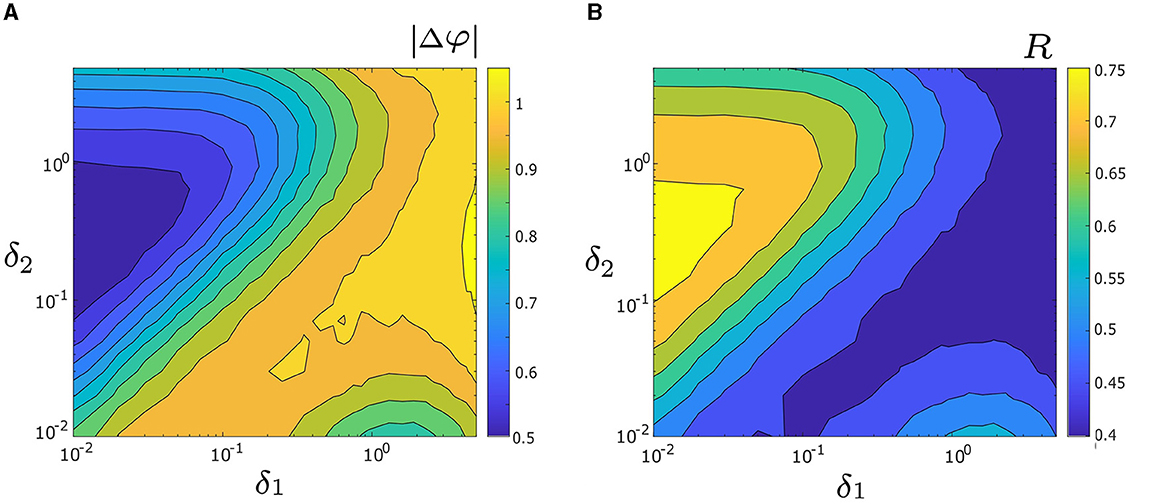
Figure 6. (A) Heat map of the mean absolute phase difference |Δφ|, as a function of noise intensities δ1 and δ2. Colder colors correspond to smaller values of |Δφ| and a decrease in |Δφ| indicates greater synchrony. The maximum synchrony is located within the dark blue triangle on the left side. The three-dimensional visualization of (A) is depicted in Supplementary Figure 1A. (B) Heat map of mean phase coherence, R, as a function of δ1 and δ2. Warmer colors correspond to larger values of R and an increase in R indicates better noise-induced synchrony. The maximum synchrony is within the yellow triangle on the left side, consistent with the observation in (A). Other parameters are: α = −0.2; γ = −0.2; ω0 = 2; ω1 = 0; λ0 = −0.5; d1 = 0.3; and d2 = 0.01.
As explained in Section 2.1, our system operates in the excitable regime, λ0 < 0, where HB1 occurs at λ0 = 0. Previous research (e.g., Yu et al., 2009, 2021) has demonstrated that in excitable networks, the distance of the control parameter from a critical point (or excitation threshold) is negatively correlated with synchronization. Moreover, in this section, we investigate the effects (if any) of the control parameter λ0 on the level of synchrony. We only use |Δφ| as a measure of synchrony since it shows results consistent with ρ and R, as demonstrated in Figures 5, 6.
We begin by evaluating |Δφ| for various λ0 values within the excitable regime, λ0 < 0, as illustrated in Figure 7 (|Δφ| vs. δ2 with fixed δ1 = 0.1). The solid blue, dashed orange, and dotted black lines correspond to λ0 = −0.03, −0.5, and −1, respectively. As observed for the blue curve in Figure 5A, all three |Δφ| curves in Figure 7A exhibit a decreasing trend until they reach a minimum value, after which they start increasing again. This suggests that the level of synchrony can be optimized by adjusting the intrinsic noise intensity δ2. Furthermore, for a fixed δ2 within the weak intensity range (e.g., δ2 < 0.5 in Figure 7A), |Δφ| is smaller when λ0 is closer to zero. This indicates that in the weak noise regime synchronization is enhanced as λ0 approaches the excitation threshold λ0 = 0 (i.e., HB1 in Figures 1, 2). Conversely, when δ2 is fixed within the strong intensity range (e.g., δ2 > 1.5 in Figure 7A), |Δφ| increases as λ0 approaches the excitation threshold, resulting in lower levels of synchrony.
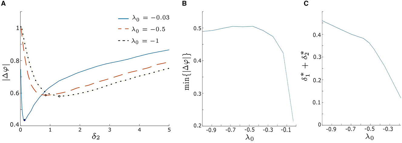
Figure 7. (A) Absolute value of the phase difference, |Δφ|, vs. noise intensity δ2 for λ0 = −0.03, −0.5, and − 1 with δ1 = 0.1. The blue solid, orange dashed, and black dotted lines correspond to λ0 = −0.03, −0.5, and − 1, respectively. Increasing λ0 leads to a decrease in the minimum value of |Δφ|, implying enhanced synchrony as λ0 approaches zero. (B) Minimum |Δφ|, denoted as min{|Δφ|}, as a function of λ0 by varying both δ1 and δ2 over from 0.01 to 5. min{|Δφ|} significantly decreases when λ0 > −0.3, suggesting a rapid improvement in synchrony as λ0 approaches zero. (C) The sum of the optimal noise intensities, , decreases as λ0 increases, indicating that smaller noise intensities are needed to achieve min{|Δφ|} as λ0 approaches zero. Other parameters are: α = −0.2; γ = −0.2; ω0 = 2; ω1 = 0; d1 = 0.3; and d2 = 0.01.
Furthermore, we observe that the minimum values of |Δφ| vary for different λ0, and the corresponding optimal noise intensities differ as well. The minimum |Δφ| values, denoted by min{|Δφ|}, are marked by black dots in Figure 7A. When λ0 is closer to the excitation threshold, our model achieves a greater degree of synchrony, and a smaller optimal δ2 is required to produce it (for fixed δ1 = 0.1). To explore this further, we plot the values of min{|Δφ|} and the sum of the optimal noise intensities, denoted , for a range of λ0 values in Figures 7B, C, respectively. For λ0 values that are relatively far from the excitation threshold (e.g., λ0 < −0.3), the curve in Figure 7B is relatively flat and the curve in Figure 7C has a relatively low slope (≈−0.332). This indicates that min{|Δφ|} and the corresponding optimal intensities remain stable over this region of λ0. Hence, it follows that small changes in λ0 do not significantly affect the synchronization of our model when λ0 is far from the threshold λ0 = 0. However, when λ0 approaches the excitation threshold (e.g., −0.5 < λ0 < 0 in Figures 7B, C), min{|Δφ|} decreases exponentially, and decreases with a steeper slope (≈ −1.84) as . These findings suggest that by shifting λ0 closer to the excitation threshold, the noise-induced synchrony of our system can be enhanced, with smaller intensities of noise required to produce this effect.
In Section 3.3, we briefly described the relationship between the necessary coupling strength and the optimal noise intensity for attaining the maximum level of synchrony. Figure 6 illustrates that when the coupling strength d1 of oscillator 1 is greater than that of oscillator 2 (d2), achieving the greatest level of synchrony requires δ1 < δ2. In this section, we investigate how uneven coupling and asymmetric noise intensities interact with one another to influence synchrony. For the sake of simplicity, we set λ0 = −0.5 and use |Δφ| to quantify synchrony.
We begin by examining the change in |Δφ| as a function of δ1 and δ2 in four disparate coupling cases: d1 ≫ d2 (e.g., d1 = 0.3 and d2 = 0.01 in Figure 6A); d1 > d2 (e.g., d1 = 0.2 and d2 = 0.1 in Figure 8A); d1 < d2 (e.g., d1 = 0.1 and d2 = 0.2 in Figure 8B), and d1 ≪ d2 (e.g., d1 = 0.01 and d2 = 0.3 in Figure 8C). The four cases are also visualized in three dimensions using surface plots and presented in Supplementary Figure 1. Both heat maps and surface plots show that |Δφ| has both a unique absolute minimum and unique local minimum which correspond to points of increased synchrony. Furthermore, each panel in Figure 8 exhibits a relatively low degree of synchrony along the line δ1 = δ2 (i.e., a relatively larger |Δφ|), which is in agreement with our results in Figure 6. These observations suggest that noise-induced synchrony tends to be maximized by asymmetric noise intensities (i.e., δ1/δ2 ≠ 1) as opposed to symmetric noise intensities (i.e., δ1/δ2 = 1).
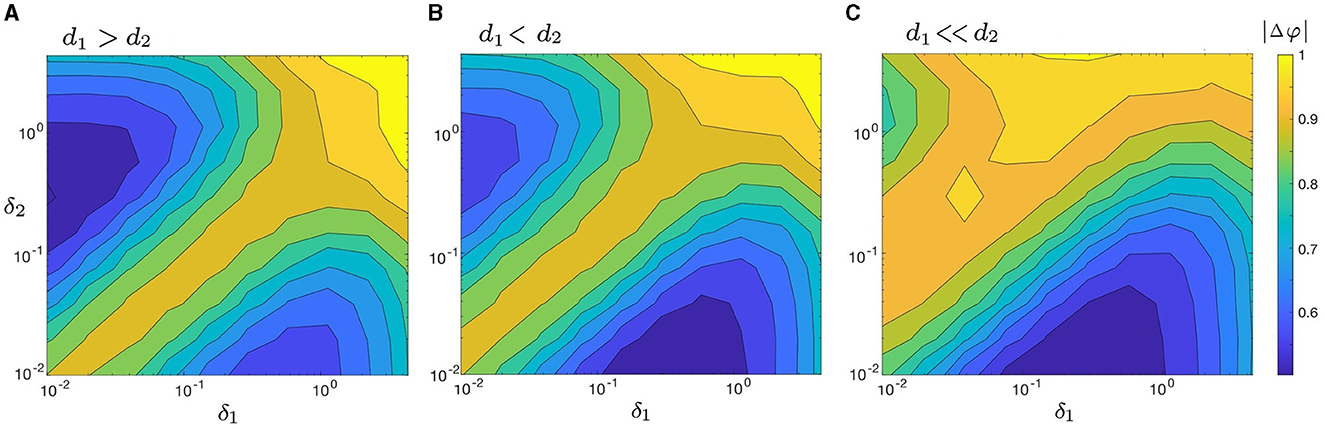
Figure 8. Heat maps of |Δφ|, as a function of δ1 and δ2 for three cases of coupling strengths: (A) d1 > d2 (with d1 = 0.2, d2 = 0.1); (B) d1 < d2 (with d1 = 0.1, d2 = 0.2); and (C) d1 ≪ d2 (with d1 = 0.01, d2 = 0.3). When d1 ≫ d2 (Figure 6A) and d1 > d2 [(A) here], the absolute minimum of |Δφ| is located on the upper left side of the heat map, where δ1 < δ2. When d1 < d2 (B) and d1 ≪ d2 (C), the absolute minimum of |Δφ| lies on the lower right side, where δ1 > δ2. The maximum synchrony varies with both δi and di, but it is never achieved when δ1 = δ2, regardless of the chosen coupling strengths. Other parameters are: α = −0.2; γ = −0.2; ω0 = 2; ω1 = 0; and λ0 = −0.5. The three-dimensional visualization of Figure 8 (surface plots) is illustrated in Supplementary Figures 1B–D.
Figures 6A, 8 further indicate that the ratio of coupling strengths, d1/d2, determines whether the minimum point of |Δφ| is local or absolute. Let abs.min{|Δφ|} denote the absolute minimum of {|Δφ|} and denote the corresponding ratio of optimal noise intensities. We find that when d1 ≫ d2 or d1 > d2, abs.min{|Δφ|} is located on the upper left (i.e., δ2 > δ1) of the heat maps in Figures 6A, 8A, with . Conversely, when d1 < d2 or d1 ≪ d2, abs.min{|Δφ|} is located on the lower right (i.e., δ1 > δ2) of the heat maps in Figures 8B, C, with . Supplementary Figure 1 provides a clear depiction of the gradual transition of abs.min{|Δφ|} from the left side (with δ1 < δ2) to the right side (with δ1 > δ2) as d1/d2 changes from larger to smaller values.
To systematically explore the interaction and effects of the noise intensities and coupling strengths on synchrony, we consider the parameter space d1, d2 ∈ [0.01, 0.3] and δ1, δ2 ∈ [0.01, 0.3], and compute abs.min{|Δφ|} and . We present the results in Figures 9A, B in the form of heat maps. The upper-left “triangle” of Figures 9A, B, where d1 < d2, corresponds to the absolute minimum points on the lower right of the heat maps in Figures 8B, C. And the lower-right “triangle” of Figures 9A, B, with d1 > d2, correspond to the absolute minimum points on the upper left of the heat maps in Figures 6A, 8A.
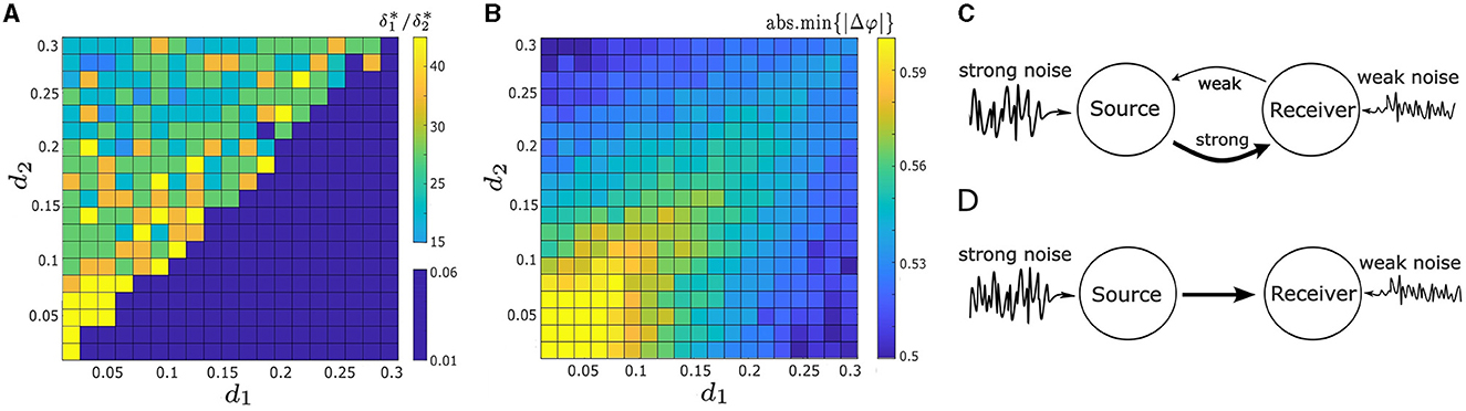
Figure 9. (A) Heat map illustrates the ratio of the optimal noise intensities, , required to minimize |Δφ|, in relation to varying both coupling strengths, d1 and d2. (B) Heat map of the absolute minimum of |Δφ|, denoted as abs.min{|Δφ|}, as a function of d1 and d2. The maximal noise-induced synchrony is not achieveed when or when d1 = d2. (C) Schematic illustration of a two-neuron motif used to enhance noise-induced synchrony. One oscillator (receiver neuron) receives robust coupling from the other oscillator (source oscillator) along with minimal noise input. Conversely, the source neuron experiences minimal coupling from the receiver neuron but substantial noise input. (D) Two-neuron motif featuring a uni-directional connection, optimizing noise-induced synchrony. Other parameters in (A, B) are: α = −0.2; γ = −0.2; ω0 = 2; ω1 = 0; and λ0 = −0.5.
Figure 9A illustrates how the choice of coupling affects . Previously, we have shown that the optimal does not equal 1 for some example pairs of d1 and d2 in Figures 6, 8. Here our result is more robust: noise-induced synchrony is never maximized at δ1/δ2 = 1 no matter the choice of coupling strengths d1 and d2. In particular, even when d1 = d2, . Figure 9A also indicates that there is a strong relationship between d1/d2 and . Specifically, when d1/d2 < 1 (upper-left “triangle”), ; whereas, when d1/d1 > 1 (lower-right “triangle”), . We also compute and for both d1/d2 cases. When d1/d2 < 1, the mean optimal noise intensities are and , which results in an average ratio of 0.3462/0.015 ≈ 23.08. And conversely, when d1/d2 > 1, and , which results in an average ratio of 0.015/0.3462 ≈ 0.043 (note that the latter ratio is the reciprocal the former).
Next, we examine how the coupling strengths influence the degree of synchrony of our system, as measured by abs.min{|Δφ|}. As in Figure 9B, abs.min{|Δφ|} exhibits symmetry with respect to the diagonal line d1 = d2. Along this line, abs.min{|Δφ|} decreases as both d1 and d2 increase. However, the smallest value of abs.min{|Δφ|} is not located along this line. This suggests that when the oscillators are symmetrically coupled, the degree of synchrony is positively correlated with the coupling strength d1 = d2, but does not lead to maximal synchronization.
In contrast, when the coupling strengths are asymmetric, abs.min{|Δφ|} decreases as the absolute difference between two coupling strength, |d1 − d2|, becomes larger, as seen in Figure 9B. Furthermore, the lowest values of abs.min{|Δφ|} occur at the upper-left and lower-right corners of Figure 9B, where one coupling strength is nearly zero and the other is the largest in the considered range. This indicates that a one-way coupling maximizes noise-induced synchronization between two coupled oscillators. Overall, synchrony is maximized when d1 ≪ d2 and δ1/δ2 ≈ 15 (the upper-left corner in Figures 9A, B), or d1 ≫ d2 and δ1/δ2 ≈ 1/15 (lower-right corner in Figures 9A, B).
Our findings indicate that the noise-induced synchrony between two coupled oscillators is enhanced in a specific scenario, as illustrated in Figure 9C. Specifically, one oscillator (referred to as the source neuron) experiences strong intrinsic noise and receives weak coupling input from the other oscillator (the receiver neuron). Conversely, the receiver neuron experiences weak intrinsic noise but receives substantial coupling input from the source neuron. The optimum noise-induced synchrony occurs in the extreme case, i.e., a uni-directional connection where the input from the receiver neuron to the source neuron is absent, as demonstrated in Figure 9D.
In many investigations exploring the noise-inuced synchronization of coupled excitable neurons, assumptions of homogeneity or near-homogeneity (e.g., common noise, symmetric noise, and equal coupling strength) are undertaken. To move beyond these seemingly unrealistic setups, our study considers a heterogeneous configuration through the introduction of independent noise sources with varying intensities and distinct coupling strengths for each neuron. We investigate the synchronous dynamics of the most representative neuron motif, characterized mathematically as a pair of coupled λ−ω oscillators in the heterogeneous context. These neural oscillators remain are quiescent in the absence of noise but may be excited by adding an intrinsic noise stimulus. Our results show that noise can induce synchronization in coupled oscillators, and this synchronization is enhanced by positioning the model closer to the bifurcation point (i.e., excitation threshold), which is consistent with previous studies (e.g., Yu et al., 2006, 2008, 2021; Thompson et al., 2012). In previous research, the noise-induced synchrony of excitable systems has been studied extensively with a focus on symmetrical interactions between oscillators (e.g., Neiman et al., 1999; Rosenblum et al., 2001; Freund et al., 2003). However, in biological systems, interactions between oscillators are often asymmetric, and thus, the assumption of symmetric interactions may be overly restrictive (Cimponeriu et al., 2003; Sheeba et al., 2009).
We investigate the impacts of two sources of heterogeneity (uneven coupling and asymmetric intrinsic noise) on the noise-induced synchrony of two coupled oscillators. Our results indicate that when the two noise intensities, δ1 and δ2, are asymmetric (i.e., δ1/δ2 ≠ 1), synchrony is promoted. We further find that the synchronization between two coupled oscillators is optimized when the absolute difference between the coupling strengths, |d1 − d2|, is as large as possible, irrespective of the coupling strengths selected. Furthermore, we have identified a correlation between the asymmetry of coupling and the intensity of noise required to maximize it. Specifically, when d1/d2 < 1, it leads to , whereas, when d1/d2 > 1, it leads to .
Our results suggest that there is a strong relationship between uneven coupling and asymmetric noise in coupled oscillators, which have potential applications in various real-world problems that exhibit asymmetry in the interactions between oscillators, such as cardio-respiratory electroencephalogram (EEG) interactions (Paluš and Stefanovska, 2003; Sheeba et al., 2009), optical communication systems, the detection of radar signals in presence of channel noise (Tsang and Lindsey, 1986), and neuronal dynamics (Singer, 1999; Sheeba et al., 2009). Moreover, our results indicate that two-neuron motifs with uni-direction (i.e., one-way) connections may exhibit a greater propensity for in-phase synchronization than two-neuron motifs with bi-directional (i.e., two-way) connections, which reinforces our understanding of the functional significance of network motifs in neuronal dynamics.
However, further investigations are necessary to explore the relationship between the ratios d1/d2 and δ1/δ2 more extensively. An extension of our current work may include investigating: (1) the role of asymmetric noise and coupling in the anti-phase synchronization of coupled oscillators by considering inhibitory coupling (i.e., di < 0 for i = 1or2); and (2) investigation of the role of noise and coupling asymmetries in other common network motifs, such as three-neuron feed-forward-loops.
The HB is one of the most common bifurcation schemes as it describes the appearance or disappearance of regular orbits with a slight change of a parameter. In this study, we employ the normal form of HB to investigate a specific scenario: noise-induced synchrony near a supercritical Hopf point. By focusing on this particular region, we aim to uncover the underlying mechanisms that lead to synchronized oscillations in physical or biological systems. Our results not only shed light on the phenomena of interest but also offer potential explanations or predictions for various systems that undergo similar shifts from a quiescent state to sustained oscillations. However, it is important to acknowledge that different systems may exhibit other bifurcation structures, necessitating further investigation to comprehensively understand their dynamic behavior.
The original contributions presented in the study are included in the article/Supplementary material, further inquiries can be directed to the corresponding author.
GJ: Formal analysis, Investigation, Methodology, Software, Visualization, Writing - original draft, Writing - review & editing. NY: Conceptualization, Formal analysis, Funding acquisition, Investigation, Methodology, Supervision, Visualization, Writing - original draft, Writing - review & editing.
GJ was supported by the Queen Elizabeth II Graduate Scholarship in Science and Technology and the Ontario Graduate Scholarship in Canada. NY received startup funding from the Faculty of Science at Toronto Metropolitan University and the Discovery Grant from the Natural Sciences and Engineering Research Council of Canada (NSERC).
The authors declare that the research was conducted in the absence of any commercial or financial relationships that could be construed as a potential conflict of interest.
All claims expressed in this article are solely those of the authors and do not necessarily represent those of their affiliated organizations, or those of the publisher, the editors and the reviewers. Any product that may be evaluated in this article, or claim that may be made by its manufacturer, is not guaranteed or endorsed by the publisher.
The Supplementary Material for this article can be found online at: https://www.frontiersin.org/articles/10.3389/fncom.2024.1347748/full#supplementary-material
Amro, R. M., Lindner, B., and Neiman, A. B. (2015). Phase diffusion in unequally noisy coupled oscillators. Phys. Rev. Lett. 115:e034101. doi: 10.1103/PhysRevLett.115.034101
Blasius, B. (2005). Anomalous phase synchronization in two asymmetrically coupled oscillators in the presence of noise. Phys. Rev. E 72:e066216. doi: 10.1103/PhysRevE.72.066216
Boccaletti, S., Latora, V., Moreno, Y., Chavez, M., and Hwang, D. U. (2006). Complex networks: structure and dynamics. Phys. Rep. 424, 175–308. doi: 10.1016/j.physrep.2005.10.009
Cimponeriu, L., Rosenblum, M. G., Fieseler, T., Dammers, J., Schiek, M., Majtanik, M., et al. (2003). Inferring asymmetric relations between interacting neuronal oscillators. Progr. Theoret. Phys. Suppl. 150, 22–36. doi: 10.1143/PTPS.150.22
Fell, J., and Axmacher, N. (2011). The role of phase synchronization in memory processes. Nat. Rev. Neurosci. 12, 105–118. doi: 10.1038/nrn2979
Freund, J. A., Schimansky-Geier, L., and Hänggi, P. (2003). Frequency and phase synchronization in stochastic systems. Chaos 13, 225–238. doi: 10.1063/1.1500497
Gambuzza, L., Gómez-Gardeñes, J., and Frasca, M. (2016). Amplitude dynamics favors synchronization in complex networks. Sci. Rep. 6:24915. doi: 10.1038/srep24915
Gang, H., Ditzinger, T., Ning, C. Z., and Haken, H. (1993). Stochastic resonance without external periodic force. Phys. Rev. Lett. 71, 807–810. doi: 10.1103/PhysRevLett.71.807
Kawasaki, M., Kitajo, K., and Yamaguchi, Y. (2018). Sensory-motor synchronization in the brain corresponds to behavioral synchronization between individuals. Neuropsychologia 119, 59–67. doi: 10.1016/j.neuropsychologia.2018.07.026
Masoliver, M., and Masoller, C. (2018). Sub-threshold signal encoding in coupled fitzhugh-nagumo neurons. Sci. Rep. 27:8276. doi: 10.1038/s41598-018-26618-8
Milo, R., Shen-Orr, S., Itzkovitz, S., Kashtan, N., and Chklovskii, D. (2002). Network motifs: simple building blocks of complex networks. Science 298, 824–827. doi: 10.1126/science.298.5594.824
Morgan, R. J., and Soltesz, I. (2008). Nonrandom connectivity of the epileptic dentate gyrus predicts a major role for neuronal hubs in seizures. Proc. Natl. Acad. Sci. U. S. A. 105, 6179–6184. doi: 10.1073/pnas.0801372105
Mormann, F., Lehnertz, K., David, P., and E. Elger, C. (2000). Mean phase coherence as a measure for phase synchronization and its application to the eeg of epilepsy patients. Phys. D 144, 358–369. doi: 10.1016/S0167-2789(00)00087-7
Neiman, A., Schimansky-Geier, L., Cornell-Bell, A., and Moss, F. (1999). Noise-enhanced phase synchronization in excitable media. Phys. Rev. Lett. 83, 4896–4899.
Paluš, M., and Stefanovska, A. (2003). Direction of coupling from phases of interacting oscillators: an information-theoretic approach. Phys. Rev. E 67:055201. doi: 10.1103/PhysRevE.67.055201
Perc, M. (2007). Effects of small-world connectivity on noise-induced temporal and spatial order in neural media. Chaos Solit. Fract. 31, 280–291. doi: 10.1016/j.chaos.2005.10.018
Perc, M., and Marhl, M. (2006). Pacemaker enhanced noise-induced synchrony in cellular arrays. Phys. Lett. A 353, 372–377. doi: 10.1016/j.physleta.2005.12.107
Pikovsky, A. (2002). Synchronization: A Universal Concept in Nonlinear Sciences. Cambridge: Cambridge University Press.
Pikovsky, A. S., and Kurths, J. (1997). Coherence resonance in a noise-driven excitable system. Phys. Rev. Lett. 78, 775–778. doi: 10.1103/PhysRevLett.78.775
Reigl, M., Alon, U., and Chklovskii, D. (2004). Search for computational modules in the C. elegans brain. BMC Biol. 2:25. doi: 10.1186/1741-7007-2-25
Rosenblum, M., Pikovsky, A., Kurths, J., Schäfer, C., and Tass, P. (2001). “Phase synchronization: from theory to data analysis,” in Neuro-Informatics and Neural Modelling, Volume 4 of Handbook of Biological Physics (Amsterdam: Elsevier Science), 279–321.
Rosenblum, M. G., Pikovsky, A. S., and Kurths, J. (2022). “Synchronization approach to analysis of biological systems,” in The Random and Fluctuating World: Celebrating Two Decades of Fluctuation and Noise Letters (Singapore: World Scientific), 335–344.
Sheeba, J. H., Chandrasekar, V. K., Stefanovska, A., and McClintock, P. V. E. (2009). Asymmetry-induced effects in coupled phase-oscillator ensembles: Routes to synchronization. Phys. Rev. E 79:e046210. doi: 10.1103/PhysRevE.79.046210
Song, S., Sjöström, P., Reigl, M., Nelson, S., and Chklovskii, D. (2005). Highly nonrandom features of synaptic connectivity in local cortical circuits. PLoS Biol. 3:e68. doi: 10.1371/journal.pbio.0030068
Thompson, W. F., Kuske, R., and Li, Y.-X. (2012). Stochastic phase dynamics of noise driven synchronization of two conditional coherent oscillators. Discr. Contin. Dyn. Syst. 32:2971. doi: 10.3934/dcds.2012.32.2971
Touboul, J. D., Piette, C., Venance, L., and Ermentrout, G. B. (2020). Noise-induced synchronization and antiresonance in interacting excitable systems: applications to deep brain stimulation in parkinson's disease. Phys. Rev. X 10:e011073. doi: 10.1103/PhysRevX.10.011073
Tsang, C.-S., and Lindsey, W. (1986). Bit synchronization in the presence of asymmetric channel noise. IEEE Trans. Commun. 34, 528–537. doi: 10.1109/TCOM.1986.1096577
Varela, F., Lachaux, J. P., Rodriguez, E., and Martinerie, J. (2001). The brainweb: phase synchronization and large-scale integration. Nat. Rev. Neurosci. 2, 229–239. doi: 10.1038/35067550
Womelsdorf, T., and Fries, P. (2007). The role of neuronal synchronization in selective attention. Curr. Opin. Neurobiol. 17, 154–160. doi: 10.1016/j.conb.2007.02.002
Yu, G., Yi, M., Jia, Y., and Tang, J. (2009). A constructive role of internal noise on coherence resonance induced by external noise in a calcium oscillation system. Chaos Solit. Fract. 41, 273–283. doi: 10.1016/j.chaos.2007.12.001
Yu, N., Jagdev, G., and Morgovsky, M. (2021). Noise-induced network bursts and coherence in a calcium-mediated neural network. Heliyon 7:e08612. doi: 10.1016/j.heliyon.2021.e08612
Yu, N., Kuske, R., and Li, Y. (2006). Stochastic phase dynamics: multiscale behavior and coherence measures. Phys. Rev. E 73:e056205. doi: 10.1103/PhysRevE.73.056205
Keywords: network motifs, coupled oscillators, synchrony, asymmetric noise, heterogeneity
Citation: Jagdev G and Yu N (2024) Noise-induced synchrony of two-neuron motifs with asymmetric noise and uneven coupling. Front. Comput. Neurosci. 18:1347748. doi: 10.3389/fncom.2024.1347748
Received: 01 December 2023; Accepted: 06 February 2024;
Published: 23 February 2024.
Edited by:
Lubica Benuskova, Comenius University, SlovakiaReviewed by:
Matjaž Perc, University of Maribor, SloveniaCopyright © 2024 Jagdev and Yu. This is an open-access article distributed under the terms of the Creative Commons Attribution License (CC BY). The use, distribution or reproduction in other forums is permitted, provided the original author(s) and the copyright owner(s) are credited and that the original publication in this journal is cited, in accordance with accepted academic practice. No use, distribution or reproduction is permitted which does not comply with these terms.
*Correspondence: Na Yu, bmF5dUB0b3JvbnRvbXUuY2E=
Disclaimer: All claims expressed in this article are solely those of the authors and do not necessarily represent those of their affiliated organizations, or those of the publisher, the editors and the reviewers. Any product that may be evaluated in this article or claim that may be made by its manufacturer is not guaranteed or endorsed by the publisher.
Research integrity at Frontiers
Learn more about the work of our research integrity team to safeguard the quality of each article we publish.