Quantification of Kuramoto Coupling Between Intrinsic Brain Networks Applied to fMRI Data in Major Depressive Disorder

Organized patterns of system-wide neural activity adapt fluently within the brain to adjust behavioral performance to environmental demands. In major depressive disorder (MD), markedly different co-activation patterns across the brain emerge from a rather similar structural substrate. Despite the application of advanced methods to describe the functional architecture, e.g., between intrinsic brain networks (IBNs), the underlying mechanisms mediating these differences remain elusive. Here we propose a novel complementary approach for quantifying the functional relations between IBNs based on the Kuramoto model. We directly estimate the Kuramoto coupling parameters (K) from IBN time courses derived from empirical fMRI data in 24 MD patients and 24 healthy controls. We find a large pattern with a significant number of Ks depending on the disease severity score Hamilton D, as assessed by permutation testing. We successfully reproduced the dependency in an independent test data set of 44 MD patients and 37 healthy controls. Comparing the results to functional connectivity from partial correlations (FC), to phase synchrony (PS) as well as to first order auto-regressive measures (AR) between the same IBNs did not show similar correlations. In subsequent validation experiments with artificial data we find that a ground truth of parametric dependencies on artificial regressors can be recovered. The results indicate that the calculation of Ks can be a useful addition to standard methods of quantifying the brain's functional architecture.

1. Introduction

The human brain is a complex adaptive system in which a stable neuronal substrate of gray and white matter architecture allows for a vast array of cognitive sets. At any moment integrative overall network interaction defines attainable cognitive sets as well as the degree of flexibility to react to outer stimuli (Sporns et al., 2004; Deco et al., 2008; Breakspear, 2017). Empirically, on the one hand a structural connectome can be described (Sporns et al., 2005), and complementary to that functional imaging allows for assessing the functional architecture which is in parts defined by processes of chemical connectivity depending on the status of the various transmitter systems of the brain (Shine et al., 2019). Different measures have been proposed to quantify the complex interplay of brain areas measured with functional magnetic resonance imaging (fMRI) including statistical measures of coherence (functional connectivity; Friston, 2011), phase coherence (Glerean et al., 2012; Deco and Kringelbach, 2016; Cabral et al., 2017), and models of first order auto-regressive representation (Liégeois et al., 2017, 2019). Still a full understanding of how a brain state arises from neuronal underpinnings of structural and chemical connectivity remains elusive. Alternative approaches might help to fill into this gap. Table 1 contains all abbreviations used in this paper.

TABLE 1

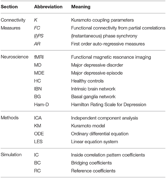
Table 1. Abbreviations.

The Kuramoto model of coupled oscillators (Okuda and Kuramoto, 1991) has been introduced to neuroscience as one potential generative model governing fluctuating oscillations in large-scale cortical circuits (Breakspear et al., 2010; Cocchi et al., 2016). The model poses that the differences in time course phases between any two oscillators are causal to phase readjustments at both ends (Okuda and Kuramoto, 1991).

While classical functional connectivity analyses look for first order statistical associations, the application of the Kuramoto model to fMRI data employs a more specific, yet simple, biophysiological model, i.e., it addresses the issue of a slow BOLD response to fast neuronal processes. As depicted in Figure 1A an event of fast neuronal firing in one region would cause an attraction of the phase of the fMRI signal in a second region receiving excitatory neuronal projections from the first one. Conversely, repetitive inhibitory impact from one region onto the other on a fast time scale would cause phase repulsion on the fMRI time scale. In this broader conceptualization, the Kuramoto coupling strengths can serve as empirical measures even without the assumption that the brain regions are perfect oscillators.

FIGURE 1

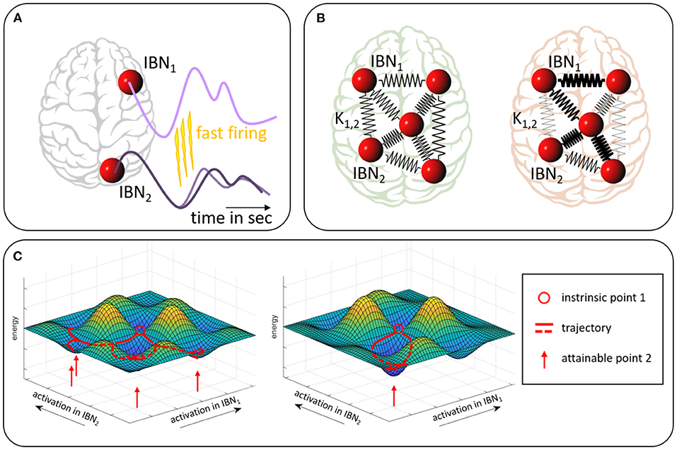
Figure 1. Sketch of the model assumption. (A) Excitatory neuronal firing from IBN₁ on a fast time scale leads to an earlier signal rise in IBN₂ which effectively means a phase readjustment in the slow BOLD time course of the targeted IBN. Conversely, inhibitory firing would lead to a phase adjustment in the form of phase repulsion. (B) Pair-wise Kuramoto phase couplings of IBNs, symbolized by spring constants (here undirected), determine network-wide dynamics and are altered in pathology (compare red vs. green). (C) Energy landscape on a very reduced subspace of only two IBNs. Different activation constellations of the two IBNs (x- and y-axis) are associated with different energy levels (z-axis). Intrinsic information flow between the IBNs favors selective co-activations and penalizes others. The red circle indicates an arbitrary intrinsic state (i.e., co-activation constellation between IBNs), red lines indicate trajectories from this state which are favored by the landscape, red arrows indicate a set of states likely to be attained under the prevailing structural and synaptic conditions. The landscape is based on the underlying neuronal and synaptic connectivity. Minor adjustments to an overall stable energy landscape (compare left and right) may impact on fast firing intensity and thereby on Kuramoto coupling parameters K_i,j. This might allow for or subdue more versatile co-activation patterns. Widely projecting transmitter systems bear the potential of widespread moderate adjustments to the energy landscape.

The overall energy landscape, which determines the likelihood of any pattern of simultaneously active brain regions (Okuda and Kuramoto, 1991; Shine, 2020), depends on the individual coupling strengths (see Figure 1B). Minor, but widespread modifications in the coupling strengths result in changes of this landscape and thereby in a notably different spectrum of co-activations. These ultimately have to be understood as different brain processes, i.e., alterations in thought and behavior. The idea is illustrated in a conceptual sketch in Figure 1C. In this view Kuramoto coupling between brain areas could for instance be changed by underlying changes in the transmitter system status which impacts on the amount of fast firing. The model, therefore, might offer a distinct complementary approach to other existing ones based on an appealing generative model.

Major depressive disorder (MD) is associated with experiences of depressed mood, with impaired cognition, energy loss, vegetative symptoms, and suicidal thoughts (American Psychiatric Association, 2013). This spectrum of diverse symptoms suggests a likely involvement of several distinct neural circuits in creating an aberrant brain state (Northoff, 2016). MD is not associated with a major focal brain lesion, but is frequently associated with alterations in synaptic, chemical rather than structural connectivity, in particular with monoamine dysfunction, which has been investigated in detail in animal and human models of depression (Cooper et al., 1991; Delgado et al., 1994; Hamon and Blier, 2013). Most antidepressants act on monoamine re-uptake mechanisms or monoamine post-synaptic receptors (Anand and Charney, 1997). Monoamine transmitter systems are mainly centrally controlled by brainstem nuclei, which exert wide spread influence via broad projections to nearly all cortico-limbic regions (Goldman-Rakic et al., 1989; Robbins and Arnsten, 2009; Jacob and Nienborg, 2018). Although they may be central to the generative mechanisms determining pathological alterations of the brain's energy landscape their direct impact on fMRI measures is difficult to establish. Therefore, a method investigating moderate but wide spread changes in the brain's functional architecture focussing on causal impact of brain regions onto each other might be of use.

In the present study we present a novel approach which consists of the direct estimation of Kuramoto coupling parameters (K) from empirical data (section 2.2). Statistical analysis is designed (section 2.4) to assess significance based not on individual coupling parameters, but on whole sets of couplings, which is in line with the underlying assumptions. The focus, therefore, shifts away from spatial localization toward modifications of the dynamics of the brain as a system. We use an exploratory data set to detect dependencies of K on clinical severity. These specific hypotheses are then tested in an entirely independent larger test data set, which underwent identical preprocessing. Specifically, within the initial exploratory analysis, we apply this method to intrinsic brain networks (IBNs) in a collective of patients with major depressive disorder (MD) and matched healthy controls, and compare it to three other measures (section 2.3): (i) functional connectivity via partial correlations (FC), (ii) phase synchrony (PS), and (iii) parameters of a first order auto-regressive model (AR). We then test if significant findings on K can be recovered in the independent test data set. We hypothesize that Ks show wide spread alterations with severity of pathology. By a set of simulations (section 4, Appendix A) we test the ability of our method to recover parametric dependencies and delineate scenarios in which parametric dependencies of Ks on external variables are accessible to the methodology.

2. Materials and Methods

2.1. Empirical Data of Resting State fMRI in Patients With Major Depressive Disorder and Healthy Controls

2.1.1. Participants

2.1.1.1. Exploratory Data Set

Data was acquired in 25 patients with recurrent MD and 25 age matched control subjects. One patient and one control had to be excluded due to image artifacts, resulting in 24 subjects per group. Mean age in the MD group was 48y [min/max: 23y/79y, 13 female], and 44y [min/max: 26y/68y, 14 female] in the control group. All patients received medication at the time of scanning. Supplementary Table 1 provides details on demographic and clinical characteristics. Participant data have been used in several previous studies (Manoliu et al., 2014; Meng et al., 2014; Ries et al., 2018, 2019). To render results of the IBN determination more robust 25 young healthy control (HC) participants (age 19–32, right handed) were included into the independent component analysis described below. All participants gave informed consent in accordance with the in-house ethics committee of the Klinikum rechts der Isar, TU Munich. Patients were recruited at the psychiatry department of the Klinikum rechts der Isar, TU Munich. Clinical assessment, including DSM IV (American Psychiatric Association, 2000) and Hamilton Rating Scale for Depression (Ham-D, Hamilton, 1960), was performed by two experienced psychiatrists [Structured Clinical Interview for DSM-IV (SCID) inter-rater reliability of 95%]. HCs were recruited by word-of-mouth advertising. MD was the primary diagnosis for all patients, with all of them meeting criteria for a current major depressive episode (MDE) with an average current episode length of 16 weeks (SD = 7), an average Ham-D score of 21.8 (SD = 7.1). The mean duration of MD was 16.72 years (SD = 10.20), the mean number of episodes 6 (SD = 3). Exclusion criteria for patients were psychotic symptoms, schizophrenia, schizo-affective disorder, bipolar disorder, and substance abuse. Exclusion criteria for all participants were pregnancy, neurological or severe internal systemic diseases, and general contraindications for MRI. All patients were medicated (for details see Meng et al., 2014) except for one patient who was free of any psychotropic medication during MRI assessment.

All participants underwent 10 min of rs-fMRI with the instruction to keep their eyes closed and not to fall asleep.

2.1.1.2. Test Data Set

All subjects were included in the study after signing an informed consent form approved by the Investigational Review Board (IRB) at Indiana University School of Medicine and at the Cleveland Clinic Foundation.

One hundred seven medication-free MD subjects and 51 HCs were recruited as part of a study of young adult MD subjects at high and low risk for bipolar disorder. Out of the 107 MD subjects 28 subjects were excluded due to excessive motion, falling asleep during scanning, incomplete or lacking data, and poor data quality. Thirty-five further subjects were excluded from the statistical analysis due to inconsistent imaging parameters, and mild symptoms of mania as assessed by a score of more than 1 on the Young Mania Rating Scale (YMRS). Out of the 51 HCs 10 subjects were excluded due to excessive motion, falling asleep during scanning, incomplete or lacking data, and poor data quality or family history of psychiatric illness. Four further subjects were excluded from statistical analysis due to inconsistent scanning parameters. Data of the extended patient data set without restrictions on YMRS and inconsistent imaging parameters were processed and included into the independent component analysis described below.

Finally, 44 patients (age: mean [min/max] 24y [18y/30y], 33 females) and 37 healthy controls (age: mean [min/max] 24y [18y/30y], 22 females) were included into the statistical analysis. See Supplementary Table 1 for a detailed presentation of demographic and clinical characteristics. A subgroup of the collective was part of a previous investigation (Wohlschläger et al., 2018). Both patients and HCs were paid $25 for screening and $75 for MRI scan. All subjects underwent a detailed structured diagnostic interview—Mini Neuropsychiatric Interview (MINI) that generated a DSM-IV diagnosis (Sheehan et al., 1997). Inclusion criteria for MD were: (1) between 15 and 30 years and able to give voluntary informed consent; (2) satisfy DSM-IV-TR criteria for MD using a structured interview; (3) never met criteria for mania or hypomania; (4) 17-item Ham-D >18 and < 25; (5) Young Mania Rating Scale (YMRS) (Young et al., 1978) score < 10; (6) satisfy safety criteria to undergo an MRI scan; (7) able to be managed as outpatients during the study, ascertained by the following—(i) Clinical Global Severity Scale < 5 i.e., moderately ill, (ii) no significant suicidal or homicidal ideation or grossly disabled.

All participants underwent 6:16 min of rs-fMRI with the instruction to keep their eyes open and to look at a fixation cross.

2.1.2. MRI Data Acquisition

2.1.2.1. Exploratory Data Set

All measurements were performed on a 3T MR scanner (Achieva, Philips, Netherland) using an 8-channel phased-array head coil. T1-weighted anatomical images were obtained from a magnetization-prepared rapid acquisition gradient echo (MPRAGE) sequence (FoV = 240 × 240 mm², 170 slices). FMRI data were obtained from a gradient echo planar imaging (EPI) sequence (TR/TE = 2, 000/35 ms, 32 slices, slice thickness = 4 mm, 300 volumes). For the additional data set of young subjects respective parameters were: T1 (FoV = 480 × 480 mm², 340 slices), fMRI (TR/TE = 2, 007/30 ms, 36 slices, slice thickness = 3 mm; 300 volumes).

2.1.2.2. Test Data Set

Measurements were acquired at Cleveland Clinic Main Campus using 3T Siemens Prisma MR Scanner. T1-weighted anatomical images were obtained from a MPRAGE sequence (FoV = 240 × 256 mm², 160 slices). FMRI data were obtained from an EPI sequence (TR/TE =2, 800/29 ms, 39 slices, slice thickness = 3.5 mm, 132 volumes). To limit the head motion scans at Cleveland Clinic were acquired with subjects fitted with a bite bar.

2.1.3. Preprocessing

During preprocessing particular care was taken to address physiological as well as movement artifacts. Effects of heart beat and breathing were quantified from the data using Physiologic Estimation by Temporal ICA (PESTICA) (Beall and Lowe, 2007), and a physiologic noise removal tool, RETROICOR (Glover et al., 2000). During this step instantaneous effects of heart beat and respiration are corrected for. Estimates of the cardiac and respiratory rates can be retrieved. There were no significant group differences in both measures. Because it has been shown that magnitude of cardiac and respiratory rate can have delayed effects within the BOLD signal (Birn et al., 2008; Chang et al., 2009) respective regressors were calculated and accounted for within the subsequent procedures (see below). Movement correction was optimized with slice-based realignment using slice-oriented motion correction (SLOMOCO) (Beall and Lowe, 2014). No significant group differences in volume-wise or slice-wise mean motion were detected (see Supplementary Table 1). Further preprocessing steps included coregistration to the T1 image, slice time correction, spatial normalization, and spatial smoothing with the full width at half maximum (FWHM) of the Gaussian filter 8 × 8 × 8 mm³ (SPM12, https://www.fil.ion.ucl.ac.uk/spm/).

2.1.4. IBN Time Course Preparation

Exploratory and test data sets of the preprocessed data were each entered into independent component analyses (ICA) and each separated into 75 spatially independent components (Calhoun et al., 2001) based on the Infomax-algorithm and implemented in the fMRI Toolbox (GIFT, http://www.icat.sourceforge.net) which was run 20 times through ICASSO to ensure stability of the estimated components. For both data sets group average components were back-projected on the single-subject data. Via multiple spatial regression 20 of the 75 independent components in the exploratory data set and 28 of the 75 independent components in the test data set were identified as neuronally meaningful IBNs with correlation coefficients above 0.15 to the spatial templates of the IBNs as described in Allen et al. (2011). The IBNs are presented in the Supplementary Figures 1, 2. Time courses from these IBNs for each subject were corrected for effects of white matter signal, and signal from the cerebrospinal fluid, and additionally for effects of the respiratory (Birn et al., 2008), and the cardiac (Chang et al., 2009) response functions, by regression. The latter two functions compensate for delayed effects of variations in respiratory and breathing rates on the BOLD signal. In order to select a frequency band affected by dynamical changes in the patient group, metastability was calculated for a range of frequency bins (Ries et al., 2019) as described in the Supplementary Material (section 1.3) (Figure 3). Frequency bin 3 displayed significant reduction in metastability in the patients. Based on this finding, time courses were bandpass filtered to a narrow frequency band of 0.05–0.075 Hz in preparation for a subsequent Hilbert transformation (Córdova-Palomera et al., 2017) using a Butterworth filter of order 7. The FC and AR measures are not based on phase analysis, therefore, the frequency range does not have to be that strongly reduced. Here the less stringent, commonly used frequency band of 0.01–0.1 Hz (Zang et al., 2007) was chosen as band pass filter.

2.2. Calculation of Kuramoto Coupling Coefficients

This section describes the methodological concepts which we will use to analyze the coupling behavior in our data sets. Table 2 gives an overview of the most important notation used in the following sections.

TABLE 2

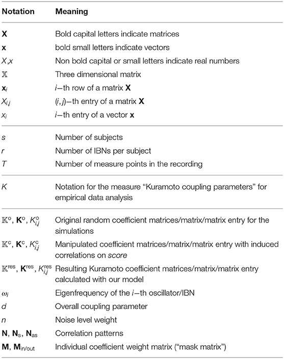
Table 2. Notation.

2.2.1. Kuramoto Model

First, we consider the Kuramoto model (KM) (Kuramoto, 1975; Acebrón et al., 2005). This is a system of ordinary differential equations (ODEs) describing the temporal change of the phases φ₁, …, φ_r of r oscillators, which are coupled by the sine of their phase differences:

$\begin{array}{l}{\dot{\phi }}_i(t)=\frac{\partial {\phi }_i(t)}{\partial t}={\omega }_i+\frac{C}{r}{\displaystyle \sum _{j=1}^r}{K}_{i,j}sin({\phi }_j(t)-{\phi }_i(t))=f(t,{\phi }_i(t))\\ i=1,\dots ,r.& (1)\end{array}$

Here, φ_i(t) is the phase angle of the i–th oscillator at time point t and ω_i is the eigenfrequency of the i-th oscillator. The only parameters in this model are the coupling coefficients K_i,j describing the connection between oscillator i and j. In this model couplings between each and every oscillator are considered, which matches our assumption of wide-spread effects and simultaneous involvement of all IBNs. The coupling strength C can be set to 1 since it is an equal scaling for the K_i,j parameters. Note, that the model can attain different forms. The choice of this form is discussed in the Supplementary Material (section 2.1).

Each subject in our data set has r time courses x(t) representing the activity in r IBNs. The use of this model for our time series data x(t) first requires the extraction of the instantaneous phases φ(t) for each time course.

2.2.2. Hilbert Transform

The Hilbert transform (Hahn, 1996) denoted by H{x(t)} returns a version of the original time series shifted by $\frac{\pi }{2}$. Considering the analytical signal x_a(t)=x(t)+i·H{x(t)}, we can then represent the time series in an amplitude-phase representation.

$\begin{array}{ll}x(t)=a(t)·cos(\phi (t))& (2)\end{array}$

with the instantaneous amplitude a(t)=|x_a(t)| and the instantaneous phase φ(t)=∠x_a(t).

2.2.3. Numerical Solution Method

The usual way of utilizing an ODE model such as the KM, is to set the model parameters (in this case the K_i,j) suitable for the domain application and subsequently calculate a solution that fulfills the model equations (i.e., the functions φ₁, …, φ_r) with a numerical solver. This has been done previously in Neuroscience (Stramaglia et al., 2017)—also for the Kuramoto model (Schmidt et al., 2015). There exist many numerical approximation methods. One of the most basic approaches is Euler's method (Epperson, 2013). The approximation of the solution is calculated step-wise according to the following rule

$\begin{array}{ll}{\phi }_i(s+1)={\phi }_i(s)+f(s,{\phi }_i(s)).& (3)\end{array}$

with the iteration steps s and s + 1 and a step size h chosen as 1. Discussion about this choice and also the choice of the Euler method as a numerical solution method can be found in the Supplementary Material (section 2.2).

In this work, we are already given phase courses from the recordings (i.e., the functions φ₁, …, φ_r). The time courses in our experiments are filtered to a very narrow frequency band. Therefore, we can model the eigen-frequencies ω_i as the mean frequency $\stackrel{-}{\omega }$ of the respective frequency band. Another option would be to estimate each eigen-frequency from the largest peak in the frequency profile of each time course via fast Fourier transform (FFT). Our codes provide both options. Unless mentioned otherwise, all our experiments were conducted using a fixed mean eigen-frequency. Given all phase and eigen-frequency values, we are able to choose a reverse engineering approach. We assume that the KM can describe synchronization or coupling respectively of our given data and utilize formula (3) to calculate the KM parameters K_i,j which optimally fit our data.

2.2.4. Goal

Our goal is the estimation of the coupling coefficients K_i,j of model (1) considering the given phase courses (φ₁(t), …, φ_r(t), t=1, …T) and eigen-frequencies (ω_i) of the IBN time series. The coefficients may be interpreted as the coupling strengths between the time series and, therefore, between the IBNs of a subject. We proceed as follows.

2.2.5. Linear Equation System

By transforming the time series x_i(t) of each IBN of a participant using the Hilbert transformation, we get an amplitude-phase representation of each time series

$\begin{array}{ll}{x}_i(t)=a_i(t)·cos({\phi }_i(t))t=0,\dots ,T-1.& (4)\end{array}$

This way we obtain the actual time course of the phases φ_i(t) of the time series x_i(t), i=1, …, r. So instead of simulating the synchronization of initial phase values of a subject's time series, we assume that synchronization of the phases is explainable by the above Kuramoto model (1). Considering the phase values φ_i(t), t=0, …, T − 1 of a single time course of a single subject and plugging in those phase values into Equation (3) leads to linear equations of the form

$\begin{array}{l}{\phi }_i(s+1)={\phi }_i(s)+{\omega }_i+\frac{1}{r}{\displaystyle \sum _{j=1}^r}{K}_{i,j}sin({\phi }_j(s)-{\phi }_i(s)),\\ s=0,\dots ,T-2.& (5)\end{array}$

In our exploratory data set, we have T = 300 measure points in the recording and each of the s = 24 subjects per group has recordings for r = 20 IBNs. Thus, we obtain 299 (# time steps) equations for 20 (# IBNs) unknown variables K_i,j, j=1, …, 20 for each IBN of each subject. This results in total in 400 coefficients K_i,j, i, j=1, …, 20 for one subject. Note again, that time steps are labeled as s=0, 1, 2, …, 299 corresponding to iterations while the values correspond to time points t=0, 2, 4, …, 598 in seconds. The equations can be rearranged to the form of a linear equation system (LES)

$\begin{array}{ll}{\text{S}}_i·{\text{k}}_i={\text{b}}_i,& (6)\end{array}$

with ${\text{S}}_i\in {ℝ}^{299\times 20}$, ${\text{k}}_i\in {ℝ}^{20}$, and ${\text{b}}_i\in {ℝ}^{299}$. The system matrix S_i will, however, have one zero column, which corresponds to the coefficient K_i,i. We have to eliminate this column in order to obtain a system matrix with full rank. Accordingly, we reduce the number of unknowns by not solving for K_i,i, but determining it instead. As it represents the coupling between an IBN to itself, we simple set the value to 1 (any constant would suffice). Thus, we will determine 380 coefficients per subject. Details about the entries of S_i and b_i as well as the derivation of the entries can be found in the Supplementary Material (section 2.3).

2.2.6. Solving the LES

Since the LES (6) is over-determined, i.e., the number of equations is larger than the number of variables, we can not simply invert the non-squared system matrix S_i. We solve the over-determined LES optimal with respect to the ℓ₂ norm by building the normal equations (Gauß, 1809; Abdulle and Wanner, 2002).

$\begin{array}{ll}{\displaystyle \underset{{Ŝ}_i}{{\displaystyle \underbrace{{\text{S}}_i^{\text{T}}{\text{S}}_i}}}}·{\widehat{\text{k}}}_i={\displaystyle \underset{{\text{b}}_i}{{\displaystyle \underbrace{{\text{S}}_i^{\text{T}}·{\text{b}}_i}}}}.& (7)\end{array}$

The symmetric matrix ${\widehat{\text{S}}}_i\in {ℝ}^{19\times 19}$ is regular and can, therefore, be inverted to obtain a unique solution ${\widehat{\text{k}}}_i\in {ℝ}^{19}$, where it holds

$\begin{array}{ll}{\Vert {\text{S}}_i·{\widehat{\text{k}}}_i-{\text{b}}_i\Vert }_{{\ell }_2}^2={\displaystyle \underset{\text{x}\in {ℝ}^{19}}{min}}{\Vert {\text{S}}_i·\text{x}-{\text{b}}_i\Vert }_{{\ell }_2}^2& (8)\end{array}$

Derivations of the normal equations to yield the optimal solution in the sense of Equation (8) are given in the Supplementary Material (section 2.4). In order to solve the equations simultaneously for all IBNs of one subject, we build a block diagonal equation matrix, and append the inhomogeneity terms resulting in

$\begin{array}{ll}\text{S}=\left(\begin{array}{cccc}{\text{S}}_1& 0& \cdots & 0\\ 0& {\text{S}}_2& \cdots & 0\\ ⋮& ⋮& \ddots & ⋮\\ 0& 0& \cdots & {\text{S}}_{20}\\ \end{array}\right)& (9)\end{array}$

$\begin{array}{ll}\text{b}=\left(\begin{array}{c}{\text{b}}_1\\ {\text{b}}_2\\ ⋮\\ {\text{b}}_{20}\end{array}\right)& (10)\end{array}$

We calculate the solution $\widehat{\text{k}}\in {ℝ}^{380}$ of the LES

$\begin{array}{ll}{\text{S}}^{\text{T}}·\text{S}·\widehat{\text{k}}={\text{S}}^{\text{T}}·\text{b}& (11)\end{array}$

by a simple matrix inversion

$\begin{array}{ll}\widehat{\text{k}}={({\text{S}}^{\text{T}}·\text{S})}^{-1}·{\text{S}}^{\text{T}}·\text{b}& (12)\end{array}$

Finally, we set the resulting Kuramoto coupling coefficients for one subject ${\text{k}}^{\mathrm{\text{res}}}:=\widehat{\text{k}}$. We perform these steps for each subject which provides us with 380 coefficients $K_{i,j}^{\mathrm{\text{res}}}$, i, j=1, …, 20, i ≠ j per individual. The vector k^res can be reshaped to a Kuramoto coupling matrix K^res of size 20 × 20 by putting the coefficient estimating the coupling between IBN i to IBN j in the (i, j)−th entry and filling up the diagonal with ones. This can nicely be visualized by a heat map (see Supplementary Figure 4 for an example visualization). Gathering all Kuramoto coupling coefficient for all subjects in a group results in a three dimensional matrix object of size s × r × r, which we term K^res. This object contains the calculated Kuramoto coupling coefficient, which are given the marker name K in Introduction (section 1), Results (section 3.1) and Discussion (section 5) in the context of the empirical data sets.

All calculations were implemented in Matlab R2018a¹. Scripts are available via the following link: https://doi.org/10.6084/m9.figshare.13352399.

2.3. Calculation of Reference Coupling Measures

2.3.1. Partial Correlations (FC)

Time course data were filtered to a frequency band of 0.01–0.1 Hz (Zang et al., 2007). Partial correlations between each and any of the IBNs were calculated from the time courses of all IBNs using Matlab.

2.3.2. Phase Synchrony (PS)

Time course data were filtered to a frequency band of 0.05–0.075 Hz (as in the calculation of K) in preparation for the subsequently conducted Hilbert transformation (Córdova-Palomera et al., 2017). PS were calculated pairwise from the phase time courses between each and any of the IBNs according to

$\begin{array}{ll}P{S}_{i,j}=\text{med}(IP{S}_{i,j}(t))=\text{med}(cos({\phi }_j(t)-{\phi }_i(t)))& (13)\end{array}$

Here, med(·) is the median function across time applied to the instantaneous phase synchrony IPS(t) (Zarghami et al., 2020) and φ_i(t) is the phase angle of the i–th oscillator at time point t given in rad.

2.3.3. Coefficients of a First Order Auto-Regressive Model (AR)

Time course data were filtered to a frequency band of 0.01–0.1 Hz (Zang et al., 2007). Calculation of the auto-regressive coefficients, including auto-regression within one and the same time course, were performed using the scripts available from Liégeois et al. (2019) according to their Equation (1):

$\begin{array}{ll}x(t)=AR\times x(t-1)+ϵ(t)& (14)\end{array}$

2.4. Statistical Analysis

2.4.1. Set-Level Statistics

We were particularly interested in wide spread changes of Ks and the control measures across the whole brain. We therefore tested whether the number of individual correlations depending on a regressor (Ham-D) were likely to occur by chance. To this, we compared the sizes of sets containing couplings with statistically significant dependencies on the regressor against the distribution of set sizes derived from random permutations of K-values.

In detail, we assessed the significance of sets of K_i,js showing moderate associations to a parametric regressor per group via the number of these association. We calculated Spearman correlations per individual coupling to a given regressor, and counted the number of significant correlation at a threshold of P_u < 0.05, uncorrected for multiple comparisons. Subsequently, all couplings were permuted within each subject of the group and we repeated the correlation procedure yielding a number of chance correlations and, therefore, chance set sizes at the threshold of P_u < 0.05. By repeating this procedure we produced a distribution of the number of chance set sizes, to which we compared the actual set size (see Figure 2). We generated a P-value from the percentage of chance set sizes larger than the actual set size. The script accounts for the fact, that matrices can be symmetric (FC, PS) or non-symmetric (K, AR). A number of 500 permutations yielded stable results for the P-values.

FIGURE 2

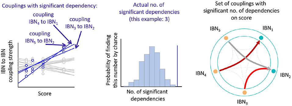
Figure 2. Analysis pipeline on empirical data. (Left) From correlations of all individual coupling parameters to a parametric score across subjects, moderately significant correlations (blue) vs. non-significant correlations (gray) are detected. (Middle) The number of these correlating couplings (“set size”) is compared to the distribution of the set sizes derived from permutations of the couplings. (Right) Sets of couplings reaching significance are displayed.

We performed similar tests on the set-level for finding sets of significant couplings versus zero and sets of significant couplings showing group differences, by replacing the correlation procedure with Wilcoxon signed rank and Wilcoxon rank sum test, respectively.

Data deviating more than two standard deviations from the mean were regarded as outliers. All procedures were implemented in Matlab including parts of the script sig_permtest.m (http://commdetect.weebly.com/).

Corrections for multiple comparisons was necessary, because we performed correlations on two regressors (Ham-D, Age) in three versions (bi-directional, positive, negative) in the patient group, amounting to a Bonferroni factor of 6. In the control group we only analyzed the age regressor in the three versions, amounting to a Bonferroni factor of 3. In all other tests of couplings versus zero or between groups we corrected the threshold for significance by a Bonferroni factor of 3 for the three directions of the test always performed. P-values reported for the test data set are not corrected for multiple comparisons.

In the exploratory data set, dependencies of coupling sets with age were found for PS in patients as well as healthy controls [MD: bi-directional (i): P_u=0.004, positive (ii): P_u=0.022, negative (iii): P_u=0.008; HC: bi-directional (i): P_u=0.036, positive (ii): P_u=0.046, negative (iii): P_u=0.092, uncorrected for multiple comparisons]. No such sets were found for K and AR. Therefore, all set-level statistics for FC and PS were corrected for age by regressing out age from each individual coupling. There was no significant dependence on sex for any coupling measure.

We investigated correlations of K with mean head motion and cardiac rate. In the patient group of the exploratory data set we detected a correlation of head motion with sets of Ks. This is discussed detail in Supplementary Material (section 4.1). There were no other significant correlations of K with movement or cardiac rate.

2.4.2. Phase Randomized Surrogates

Significant dependence of the coupling measures K and PS on regressors was additionally assessed by using phase randomized surrogates to eliminate any estimation bias. Time course phases were randomized while preserving their power spectra by the following steps (Ponce-Alvarez et al., 2015): (i) each time course underwent Fourier transformation, (ii) the phase values were replaced by values from a random uniform distribution between −π and π, and (iii) in order to return to the time domain an inverse Fourier transform was applied. K and PS calculation was applied to the phase randomized data sets. Significance of set-level correlation was tested against 500 phase randomizations.

3. Results

3.1. Results on Empirical fMRI Data in Patients With Major Depression and Healthy Controls

3.1.1. Sets of Ks Show Particular Dependence on Disease Severity

We wanted to see if there were sets of specific Ks exhibiting group differences or parametric dependencies in the exploratory data set. We used a permutation approach to estimate the probability of the number of couplings showing moderate dependence on either group or a parametric regressor occurring by chance (see Figure 2). This approach allows for detecting parametric dependencies with opposite signs in different couplings. The tests were, therefore, performed separately (i) irrespective of the direction of associations between couplings and parametric regressor or group, (ii) for positive associations, or (iii) negative associations.

With regards to group differences, none could be detected from the Ks. FC provided a set of couplings being at trend (P_c=0.063) in the contrast of type (ii), i.e., they displayed higher values in the patient group than in controls (see Supplementary Figure 8, section 4.2). No other significant or trending sets were found.

Contrasting to the lack of overall group difference, Ks yielded sets of couplings displaying significant parametric dependence on the regressor of interest in the patient group.

Sets of Ks were significantly depending on the Ham-D score in the patient group (see Figures 3A,B and Table 3, showing the uncorrected P-values). The dependence was mainly driven by a positive correlation of type (ii) (P_c=0.012), meaning that Ks increased with higher disease severity, but a set including both ways of dependence, i.e., of type (i) was also significant (P_c=0.006). The set with negative dependence on Ham-D of type (iii) was not significant (P_c=0.096). We checked for set-level significance of the dependence on the Ham-D score when the eigenfrequencies in equation (1) are calculated from the data. This method yielded very similar results (i) P_c=0.012, (ii) P_c=0.036, (iii) P_c=0.11.

FIGURE 3

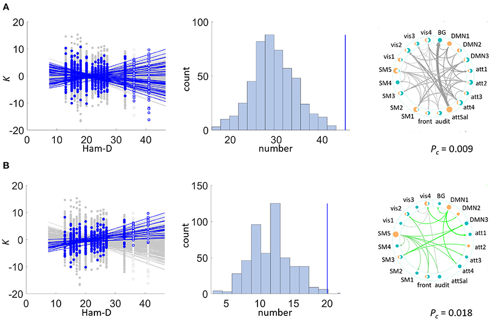
Figure 3. Set-level results. Sets of couplings of statistically significant size were detected in the exploratory data set within the patient group: K significantly depended on Ham-D in (A) the bi-directional test, mainly driven by (B) positive correlations. Left side plots depict the individual significant correlations of couplings on the regressor in blue and in gray otherwise. Note that indicated regressions in this figure were fitted to data excluding outliers (non filled markers). Middle plots depict the chance distribution on set sizes, with the actual data indicated by the blue vertical line. The right plot displays those connections constituting the significant set. Color varies with direction of correlation: bi-directional (grey), positive (green), line width scales with correlation coefficient ρ. Dots marking the IBNs are two-fold for outbound (orange) and inbound (teal) couplings, scaling in size with overall coupling strength toward all other IBNs. (A) Patient group: K vs. Ham-D. (B) Patient group: K vs. Ham-D (positive dependence).

TABLE 3

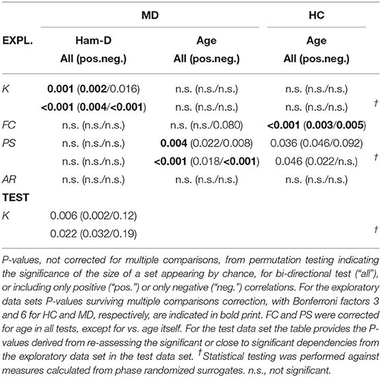
Table 3. Set level statistics.

All other analyses of FC, PS, and AR in patients and controls yielded no significant results in the dependence on Ham-D.

A significant negative correlation was found between the coupling K from the salience network onto the basal ganglia network (P_c=0.002) to Ham-D after rigorous Bonferroni correction for 380 multiple comparisons. This coupling was the only one showing a significant dependence on a score under investigation.

The re-assessment of set dependence on Ham-D in the test data set shows that the association of K to this external regressor can be recovered in the test data set.

4. Validation

The K couplings did not significantly differ from zero. Nevertheless, on a set level, dependencies to clinical severity scores could be detected in two independent empirical data sets. As an additional validation of the capabilities of our novel method, we conducted experiments with synthetically generated data. More specifically, we simulated phase courses, where we induce a dependence in the data generating coupling parameters on an independent score. Our hypothesis is, that our model should be able to detect these dependencies in the generated data. The purpose of these experiments is not to prove our method superior in comparison to other methods, but they should serve as a proof of concept, that induced dependencies can be recovered by our method.

4.1. The Simulation Model

We generate a synthetic data set for s subjects with r IBNs and T measure points each. We utilize the Kuramoto model to simulate the data, but we alter model (1) in various aspects to fit our purpose of generating phase courses. The simulated phase courses for one subject are the solution functions of the following Kuramoto model:

$\begin{array}{l}{\dot{\phi }}_i(t)=\frac{\partial {\phi }_i(t)}{\partial t}\\ ={\omega }_i+\frac{d}{r}{\displaystyle \sum _{j=1}^r}{K}_{i,j}·M_{i,j}·sin({\phi }_j(t)-{\phi }_i(t))+n·{\epsilon }_i(t)\\ i=1,\dots ,r.& (15)\end{array}$

As shown several parameters are included in the model now. First, we include eigen-frequencies ω_i for the oscillators. These are the driving forces hindering synchronization. The coupling coefficients K_i,j are the second forces determining synchronization behavior between each two oscillators i and j, i.e., K ∈ ℝ^r×r. The parameter d is a positive weight for the coupling coefficients, which acts equally on all coefficients and can be seen as an overall coupling strength. The additional weight M_i,j acts individually on each single coefficient, i.e., M ∈ ℝ^r×r. Furthermore, we include noise ε_i(t) in our model which is also weighted with an intensity level n.

To obtain simulated phase courses, we have to solve the system of ODEs. As the numerical solver of the ODE system, we choose not to work with the same as when calculating the coefficients (i.e., Euler's method). This prevents to simply get out what we put in. The solver used for the simulations is the classical Runge-Kutta algorithm (Schwarz and Köckler, 2011) also called RK-4. Providing initial values φ_i(0), i=1, …, r, the Runge Kutta method iteratively yields the phase courses. A detailed formulation of the RK-4 method is given in the Supplementary Material (section 3.1).

4.2. Simulation Procedure

For best possible comparability, we generate 20 time courses with 300 time points for 24 subjects. Therefore, we have to provide our data generating pipeline with the parameters as explained above. This includes matrices Ω ∈ ℝ^20×24 and ${\Phi }_0\in {ℝ}^{20\times 24}$ containing the 20 eigenfrequencies and initial phase values for each subject—which are both randomly initialized—, the weight matrix M ∈ ℝ^20×20, and the weights d ∈ ℝ⁺ and n ∈ ℝ⁺ for the coefficients and noise. We randomly initialize coupling coefficient matrices K ∈ ℝ^20×20 and an independent score value s ∈ ℝ (representing the Ham-D) for each subject. Across subjects, the coefficients will not be significantly correlated with this independent score, but we can manipulate each subjects coefficient matrix, such that a certain portion of the coefficients shows very high positive or negative correlation (see Figure 4A). By inserting dependencies on s for specific coefficients, this results in a correlation pattern, as can be seen in Figure 4B, where coefficients between regions from 1 to 13 show distinct correlations compared to others. The resulting manipulated coefficient matrices for all subjects K^c ∈ ℝ^24×20×20 are then also provided for the data generating procedure. An example of a generated phase course can be seen in Supplementary Figure 5.

FIGURE 4

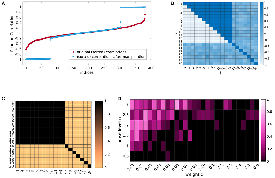
Figure 4. One exemplary result of the simulation procedure. By inserting dependencies on the data generating coupling coefficients (A) we can generate a certain correlation pattern (B). Emphasizing the influence of the significant couplings in the data generating process (C) allows to retrieve the dependencies with our method (D), when the noise to data ratio is in a certain range. (A) Correlations in ascending order for the random initial coefficients and after explicit insertion of parametric dependence. (B) Correlation pattern. (C) Weight matrix M. (D) Median P-values over the six runs for all (n, d) combinations. (P < 0.05 black).

For the 24 × 20 × 300 generated phase course data a Kuramoto coupling coefficient matrix is calculated for each subject with our Kuramoto coupling estimation model, which results in 24 matrices of size 20 × 20 (K^res). To account for the randomness in the initialization of Ω and Φ₀, we repeat the simulation pipeline for six different random phase and eigenvalue initializations and perform evaluations in account of these six runs, i.e., medians of P-values. We equidistantly set d and n within a limited value ranges and make calculations with all combinations of theses two parameters while keeping the other parameters fixed. The simulation process is quite run time intensive, therefore, we choose the number of runs to stay within a moderate run time but at the same time account to a certain degree for the randomness of the initialization. For the cluster permutation test on the resulting K^res, bi-directional correlations were considered with a number of 100 permutations.

4.3. Exemplary Result on Simulated Data

One result can be seen in Figure 4D. Each cell of the heatmap shows the median P-value of the cluster permutation test over the six runs for one combination of (n, d). The correlation pattern of the data generating coupling coefficients corresponds to Figures 4A,B, respectively. The weights in M are chosen as shown in Figure 4C, i.e., couplings are only considered in the data generation, if they show a significant correlation. As we can observe, the induced dependence on the independent score s can indeed be recovered, when the relation of noise to coupling is in a certain range.

In Appendix A, the full simulation design, parameter choices, pipeline, and results are explained in detail. Additional results are also given in the Supplementary Material.

5. Discussion

In the present study we showed that Kuramoto coupling parameters estimated from empirical data relate to a clinical scores indicating disease severity in patients with major depressive disorder. The findings acquired from the K-values differ qualitatively from findings with other methods for quantification of functional connectivity and, therefore, rather provide complementary information. While the variability within single K-values is minor, significantly larger sets of Ks relate to external scores. The findings are in line with the initial hypothesis which puts wide-spread coupling changes into context with chemical connectivity alterations at the synapses. The data provide an initial indication that parametric changes of the K-values can be discussed in context of pathological alterations of brain function in major depressive disorder (MD). By analyzing artificial data with a ground truth of parametric dependence in the couplings, we prove the ability of our analysis pipeline to recover this dependence within a reasonable parameter space of the model.

A number of recent studies highlight the explanatory power of following the trajectories of fMRI co-activation patterns from time point to time point via analysis of inter-regional connectivity measures (Gu et al., 2015; Braun et al., 2018; Liégeois et al., 2019). Gu et al. (2015) analyze how activity spread along a known structural connectome in a step-wise re-iterated way favors easy to reach states of co-activation patterns over hard to reach states. While this analysis excludes variability due to the impact of chemical transmission in activity flow, it demonstrates that co-activation states observed from fMRI can, in principle, be tracked back to the magnitude of activity flow among the whole set of brain areas from one iteration step to the next. Relating to the latter concept, Liégeois et al. (2019) show in a recent study that parameters estimated for the first order auto-regressive model from fMRI data possess a much higher capacity of explaining variance in behavioral data than a static model. For this, they used a large data set of resting state fMRI data and behavioral scores from the Human Connectome Project. Similarly in dementia, analysis of dynamic fluctuations yields more specific results than analysis of static functional connectivity (Moguilner et al., 2021). Following an alternative approach, parameters of the Ising model can be estimated from empirical data (Nguyen et al., 2017) in an application which is particularly apt for processes on the neuronal level based on binary processes of firing vs. no firing or brain states under anesthesia which involve cortical up- and down-states.

Within the present study we modified the step-wise strategy for analyzing trajectories by replacing actual activity percolation between brain regions over a time scale of seconds by a different model of spring-like attraction/repulsion between time courses of different brain regions by estimating the respective (directed) spring constants as Kuramoto coupling parameters. By this, we attempt to capture effects of fast neuronal firing on slow fMRI signal. The Kuramoto model has been used in many fields of research to investigate synchronization behavior as it is the most popular and most studied model for this phenomenon. The model can take on many different forms by adding or leaving out parameters. We decided to choose Euler's method for the following reasons: for once, it is the simplest method. Furthermore, we only consider a very short time span (T=300) alleviating stability issues, but foremost, we do not use the model for solution generation/simulation but for coefficient estimation. Therefore, the method is appropriate. For future work, however, other methods like the trapezoid method, implicit Euler's method or Runge-Kutta methods could be considered as well. When solving the linear equation system, the solution does not exist a-priori, since the number of equations will in general not be equal to the number of unknown variables. Ill-posedness in the sense that we have less equations than unknown variables will hardly occur, since this would mean that we have less measure points from the recordings than we have IBNs (In our case this meant, that we have <20 measure points, which further meant that our recording was less than about 40 s long). For the over-determined case, however, we need a strategy to find a unique solution that is optimal in a certain sense. The common approach is to solve such problems by finding the best solution in a least-squared error sense. The problem could be proposed in a more general manner, such that different norms than the ℓ₂-norm are possible. However, interpretability is more difficult in other spaces and distances than Euclidean spaces. Therefore, we solve our problem with the normal equations optimizing the ℓ₂-norm, although other approaches could also be considered in the future.

We show a correlation of the Ham-D score, assessing clinical disease severity, to K, which can very clearly be confirmed in the test data set. The nature of the correlation in exploratory as well as test data set is bipartite with a positive and a negative contribution. Positive correlation indicates that the amplitudes in a set of K values increase with increasing disease severity and vice versa. All IBNs included into the analysis contribute to the dependence on Ham-D (except for one in the exploratory data set) indicating a broad change within the inter-regional communication in clinically severe states. In the exploratory data set the directed coupling from the salience network onto the basal ganglia network shows a strong negative correlation to Ham-D. A tendency of a reduced input from the salience network into the basal ganglia matches well with hypotheses of compromised reward processing and anhedonia which is discussed in combination with the dopamine dysregulation hypothesis (Szczypiński and Gola, 2018; Whitton et al., 2020). The correlation of this particular coupling to Ham-D though is not reproduced in the test data set. Our results indicated that clinical severity of MD is associated to a mild change of cross-regional IBN interactions across the whole cortex and sub-cortex.

All our analyses aimed at wide-spread changes. We were able to retrieve global patterns of dependence. The sensitivity of the approach to localized focal changes would need to be addressed with a different appropriate data set.

Using a simulation experiment we provide a proof of principle that our method is able to recover a ground truth, in which a large number of K_i,js depend on an artificial external regressor. Notably, this parametric dependence is not associated to a systematic deviation of the K_i,js from zero. The simulations indicated that increased overall Kuramoto coupling facilitates the re-discovery of the coupling from the data. Conversely, an increasing noise level decreases the ability of our method to recover the ground truth (Supplementary Figure 3). A stronger directional bias in the couplings as well as a strong contrast in coupling dependence on the external regressor between an intrinsically coupled cluster versus the outside of the cluster, also benefit the detection of the parametric dependence. Notably, we only investigated one type of ground truth, although the artificial data simulation leaves a lot of options for design choices. The size of the generated data set was chosen to allow for comparability to the empirical exploratory data set. Also the choices for the eigenfrequencies and the magnitude of the coupling coefficients for the simulation was guided by the empirical data. The magnitude of the coefficients has subordinate impact, as this can—to a certain degree—later be scaled with the appropriate weight d.

The most interesting design choices concern the correlation pattern shape N. The possibilities here are highly diverse. First, the shape itself can be varied, i.e., which IBNs are involved and in which constellation. Additionally, the number of IBNs within the network, the intensity, pattern, and trend (“gradual progression” vs. “plateau” as for our experiments) of the correlations might be altered. Also the mask matrices used in our synthetic data experiments are only a choice of many more possible variations.

The power of our analysis pipeline for recovering the ground truth of actually parametrically manipulated couplings was limited in the considered simulation settings. Most positives were found in the “boundary” group of couplings, which crossed from one IBN, affected by parametrically dependent coupling to other regions, to another IBN, not affected by any parametrically dependent coupling to other regions. For the analysis of empirical data sets this implies that the reliability of recovering the exact couplings is low, which are actually parametrically dependent on the regressor under concern. More reliable information can be retrieved from the IBNs involved in the set themselves rather than the couplings. We would like to emphasize, that the proposed simulation pipeline and the presented results should be seen as a proof of concept, that it is possible to retrieve parametric dependencies, rather than a validation procedure, since it is impossible to have access to the ground truth of a real world data set. It is important to note, that we did find the induced dependencies in certain scenarios despite the large amount of possible parameter combinations, which supports that we did not find this by chance.

Our approach allows for an estimate of Kuramoto coupling parameters from empirical data and therefore contrasts with other studies which apply generative models in order to simulate and study arising activity dynamics, which are subsequently put in relation to empirical data. This kind of approaches has, e.g., been followed employing the Kuramoto model (Breakspear et al., 2010; Sadilek and Thurner, 2015; Schmidt et al., 2015), the Ising model (Stramaglia et al., 2017), and other spin glass models (Hudetz et al., 2014).

6. Conclusion

In summary, we present a novel method for analyzing functional connectivity from fMRI resting state data. Our initial analysis on empirical data indicates that the method provides novel results, which are complementary to other methods established in the field. The focus of the presented analysis pipeline lies on assessing wide spread connectivity changes relating to the brain state and might be useful in the analysis of the relation to slow changing chemical connectivity. The results proved to be robust to a re-test in an entirely independent data set. We further support the validity of our empirical findings by using simulated data, containing a ground truth, in that we show the ability of the method to retrieve this ground truth. Future studies are needed to extend and validate our findings.

Data Availability Statement

The original contributions presented in the study are publicly available. This data can be found here: https://doi.org/10.6084/m9.figshare.13352399.

Ethics Statement

The studies involving human participants were reviewed and approved by the in-house Ethics Committee of the Klinikum rechts der Isar, TU Munich for the exploratory data set and by the Investigational Review Board (IRB) at Indiana University School of Medicine and at the Cleveland Clinic Foundation for the test data set. The patients/participants provided their written informed consent to participate in this study.

Author Contributions

LB: methodology, software, data curation, writing, and visualization. FH, CJ, and MH: validation, investigation, and data curation. PG: supervision. AA: resources and supervision. CP: writing—review and editing and supervision. AW: conceptualization, methodology, software, formal analysis, resources, data curation, writing, and visualization. All authors contributed to the article and approved the submitted version.

Conflict of Interest

The authors declare that the research was conducted in the absence of any commercial or financial relationships that could be construed as a potential conflict of interest.

Publisher's Note

All claims expressed in this article are solely those of the authors and do not necessarily represent those of their affiliated organizations, or those of the publisher, the editors and the reviewers. Any product that may be evaluated in this article, or claim that may be made by its manufacturer, is not guaranteed or endorsed by the publisher.

Acknowledgments

Amit Anand was supported by grant number R01MH093420. We thank Dr. Mario Archila Melendez for his helpful suggestions.

Supplementary Material

The Supplementary Material for this article can be found online at: https://www.frontiersin.org/articles/10.3389/fncom.2022.729556/full#supplementary-material

Footnote

1. ^https://www.mathworks.com/.

References

Abdulle, A., and Wanner, G. (2002). 200 years of least squares method. Elemen. Math. 57, 45–60. doi: 10.1007/PL00000559

CrossRef Full Text | Google Scholar

Acebrón, J. A., Bonilla, L. L., Pérez Vicente, C. J., Ritort, F., and Spigler, R. (2005). The Kuramoto model: a simple paradigm for synchronization phenomena. Rev. Mod. Phys. 77, 137–185. doi: 10.1103/RevModPhys.77.137

PubMed Abstract | CrossRef Full Text | Google Scholar

Allen, E. A., Erhardt, E. B., Damaraju, E., Gruner, W., Segall, J. M., Silva, R. F., et al. (2011). A baseline for the multivariate comparison of resting-state networks. Front. Syst. Neurosci. 5, 2. doi: 10.3389/fnsys.2011.00002

PubMed Abstract | CrossRef Full Text | Google Scholar

American Psychiatric Association (2000). Diagnostic and Statistical Manual of Mental Disorders. Washington, DC: Am Psychiatric Association.

Google Scholar

American Psychiatric Association (2013). Diagnostic and Statistical Manual of Mental Disorders. Washington, DC: Am Psychiatric Association. doi: 10.1176/appi.books.9780890425596

PubMed Abstract | CrossRef Full Text | Google Scholar

Anand, A., and Charney, D. (1997). Depression: Neurobiological, Psychopathological and Therapeutic Advances. London: John Wiley & Sons Ltd.

Beall, E. B., and Lowe, M. J. (2007). Isolating physiologic noise sources with independently determined spatial measures. NeuroImage 37, 1286–1300. doi: 10.1016/j.neuroimage.2007.07.004

PubMed Abstract | CrossRef Full Text | Google Scholar

Beall, E. B., and Lowe, M. J. (2014). SimPACE: Generating simulated motion corrupted BOLD data with synthetic-navigated acquisition for the development and evaluation of SLOMOCO: a new, highly effective slicewise motion correction. NeuroImage 101, 21–34. doi: 10.1016/j.neuroimage.2014.06.038

PubMed Abstract | CrossRef Full Text | Google Scholar

Birn, R. M., Smith, M. A., Jones, T. B., and Bandettini, P. A. (2008). The respiration response function: the temporal dynamics of fMRI signal fluctuations related to changes in respiration. NeuroImage 40, 644–654. doi: 10.1016/j.neuroimage.2007.11.059

PubMed Abstract | CrossRef Full Text | Google Scholar

Braun, U., Schaefer, A., Betzel, R. F., Tost, H., Meyer-Lindenberg, A., and Bassett, D. S. (2018). From maps to multi-dimensional network mechanisms of mental disorders. Neuron 97, 14–31. doi: 10.1016/j.neuron.2017.11.007

PubMed Abstract | CrossRef Full Text | Google Scholar

Breakspear, M. (2017). Dynamic models of large-scale brain activity. Nat. Neurosci. 20, 340–352. doi: 10.1038/nn.4497

PubMed Abstract | CrossRef Full Text | Google Scholar

Breakspear, M., Heitmann, S., and Daffertshofer, A. (2010). Generative models of cortical oscillations: neurobiological implications of the Kuramoto model. Front. Hum. Neurosci. 4, 190. doi: 10.3389/fnhum.2010.00190

PubMed Abstract | CrossRef Full Text | Google Scholar

Cabral, J., Vidaurre, D., Marques, P., Magalh aes, R., Silva Moreira, P., Miguel Soares, J., et al. (2017). Cognitive performance in healthy older adults relates to spontaneous switching between states of functional connectivity during rest. Sci. Rep. 7, 1–13. doi: 10.1038/s41598-017-05425-7

PubMed Abstract | CrossRef Full Text | Google Scholar

Calhoun, V. D., Pearlson, G. D., and Pekar, J. J. (2001). Spatial and temporal independent component analysis of functional MRI data containing a pair of task-related waveforms. Hum. Brain Mapp. 13, 43–53. doi: 10.1002/hbm.1024

PubMed Abstract | CrossRef Full Text | Google Scholar

Chang, C., Cunningham, J. P., and Glover, G. H. (2009). Influence of heart rate on the BOLD signal: the cardiac response function. NeuroImage 44, 857–869. doi: 10.1016/j.neuroimage.2008.09.029

PubMed Abstract | CrossRef Full Text | Google Scholar

Cocchi, L., Sale, M. V., Gollo, L. L., Bell, P. T., Nguyen, V. T., Zalesky, A., et al. (2016). A hierarchy of timescales explains distinct effects of local inhibition of primary visual cortex and frontal eye fields. eLife 5, e73456. doi: 10.7554/eLife.15252.024

PubMed Abstract | CrossRef Full Text | Google Scholar

Cooper, J., Bloom, F., and Roth, R. (1991). The Biochemical Basis of Neuropharmacology. New York, NY: Oxford University Press.

Google Scholar

Córdova-Palomera, A., Kaufmann, T., Persson, K., Alnæs, D., Doan, N. T., Moberget, T., et al. (2017). Disrupted global metastability and static and dynamic brain connectivity across individuals in the Alzheimer's disease continuum. Sci. Rep. 7, 40268. doi: 10.1038/srep40268

PubMed Abstract | CrossRef Full Text

Deco, G., Jirsa, V. K., Robinson, P. A., Breakspear, M., and Friston, K. (2008). The dynamic brain: from spiking neurons to neural masses and cortical fields. PLoS Comput. Biol. 4:e1000092. doi: 10.1371/journal.pcbi.1000092

PubMed Abstract | CrossRef Full Text | Google Scholar

Deco, G., and Kringelbach, M. L. (2016). Metastability and coherence: extending the communication through coherence hypothesis using a whole-brain computational perspective. Trends Neurosci. 39, 125–135. doi: 10.1016/j.tins.2016.01.001

PubMed Abstract | CrossRef Full Text | Google Scholar

Delgado, P. L., Price, L. H., Miller, H. L., Salomon, R. M., Aghajanian, G. K., Heninger, G. R., et al. (1994). Serotonin and the neurobiology of depression: effects of tryptophan depletion in drug-free depressed patients. Arch. Gen. Psychiatry 51, 865–874. doi: 10.1001/archpsyc.1994.03950110025005

PubMed Abstract | CrossRef Full Text | Google Scholar

Epperson, J. F. (2013). An Introduction to Numerical Methods and Analysis. Hoboken, NJ: John Wiley and Sons.

Google Scholar

Friston, K. J. (2011). Functional and effective connectivity: a review. Brain Connect. 1, 13–36. doi: 10.1089/brain.2011.0008

PubMed Abstract | CrossRef Full Text | Google Scholar

Gauß, C. F. (1809). Theoria motus corporum coelestium. Rev. Mod. Phys. 7, 1–288.

Google Scholar

Glerean, E., Salmi, J., Lahnakoski, J. M., Jääskeläinen, I. P., and Sams, M. (2012). Functional magnetic resonance imaging phase synchronization as a measure of dynamic functional connectivity. Brain Connect. 2, 91–101. doi: 10.1089/brain.2011.0068

PubMed Abstract | CrossRef Full Text | Google Scholar

Glover, G. H., Li, T., and Ress, D. (2000). Image-based method for retrospective correction of physiological motion effects in fMRI: RETROICOR. Magn. Reson. Med. 44, 162–167. doi: 10.1002/1522-2594(200007)44:1<162::AID-MRM23>3.0.CO;2-E

PubMed Abstract | CrossRef Full Text | Google Scholar

Goldman-Rakic, P. S., Leranth, C., Williams, S. M., Mons, N., and Geffard, M. (1989). Dopamine synaptic complex with pyramidal neurons in primate cerebral cortex. Proc. Natl. Acad. Sci. U.S.A. 86, 9015–9019. doi: 10.1073/pnas.86.22.9015

PubMed Abstract | CrossRef Full Text | Google Scholar

Gu, S., Pasqualetti, F., Cieslak, M., Telesford, Q. K., Yu, A. B., Kahn, A. E., et al. (2015). Controllability of structural brain networks. Nat. Commun. 6, 1–10. doi: 10.1038/ncomms9414

PubMed Abstract | CrossRef Full Text | Google Scholar

Hahn, S. L. (1996). “Hilbert transforms in signal processing,” in Artech House Signal Processing Library (Boston, MA: Artech House).

Hamilton, M. (1960). A rating scale for depression. J. Neurol. Neurosurg. Psychiatry 23, 56–62. doi: 10.1136/jnnp.23.1.56

PubMed Abstract | CrossRef Full Text | Google Scholar

Hamon, M., and Blier, P. (2013). Monoamine neurocircuitry in depression and strategies for new treatments. Prog. Neuro-Psychopharmacol. Biol. Psychiatry 45, 54–63. doi: 10.1016/j.pnpbp.2013.04.009

PubMed Abstract | CrossRef Full Text | Google Scholar

Hudetz, A. G., Humphries, C. J., and Binder, J. R. (2014). Spin-glass model predicts metastable brain states that diminish in anesthesia. Front. Syst. Neurosci. 8, 234. doi: 10.3389/fnsys.2014.00234

PubMed Abstract | CrossRef Full Text | Google Scholar

Jacob, S. N., and Nienborg, H. (2018). Monoaminergic neuromodulation of sensory processing. Front. Neural Circuits 12, 51. doi: 10.3389/fncir.2018.00051

PubMed Abstract | CrossRef Full Text | Google Scholar

Kuramoto, Y. (1975). “Self-entrainment of a population of coupled non-linear oscillators,” in International Symposium on Mathematical Problems in Theoretical Physics, ed H. Araki (Berlin; Heidelberg: Springer), 420–422. doi: 10.1007/BFb0013365

CrossRef Full Text | Google Scholar

Liégeois, R., Laumann, T. O., Snyder, A. Z., Zhou, J., and Yeo, B. T. (2017). Interpreting temporal fluctuations in resting-state functional connectivity MRI. NeuroImage 163, 437–455. doi: 10.1016/j.neuroimage.2017.09.012

PubMed Abstract | CrossRef Full Text | Google Scholar

Liégeois, R., Li, J., Kong, R., Orban, C., Van De Ville, D., Ge, T., et al. (2019). Resting brain dynamics at different timescales capture distinct aspects of human behavior. Nat. Commun. 10, 2317. doi: 10.1038/s41467-019-10317-7

PubMed Abstract | CrossRef Full Text | Google Scholar

Manoliu, A., Meng, C., Brandl, F., Doll, A., Tahmasian, M., Scherr, M., et al. (2014). Insular dysfunction within the salience network is associated with severity of symptoms and aberrant inter-network connectivity in major depressive disorder. Front. Hum. Neurosci. 7, 930. doi: 10.3389/fnhum.2013.00930

PubMed Abstract | CrossRef Full Text | Google Scholar

Meng, C., Brandl, F., Tahmasian, M., Shao, J., Manoliu, A., Scherr, M., et al. (2014). Aberrant topology of striatum's connectivity is associated with the number of episodes in depression. Brain 137(Pt 2), 598–609. doi: 10.1093/brain/awt290

PubMed Abstract | CrossRef Full Text | Google Scholar

Moguilner, S., García, A. M., Perl, Y. S., Tagliazucchi, E., Piguet, O., Kumfor, F., et al. (2021). Dynamic brain fluctuations outperform connectivity measures and mirror pathophysiological profiles across dementia subtypes: a multicenter study. NeuroImage 225, 117522. doi: 10.1016/j.neuroimage.2020.117522

PubMed Abstract | CrossRef Full Text | Google Scholar

Nguyen, H. C., Zecchina, R., and Berg, J. (2017). Inverse statistical problems: from the inverse ising problem to data science. Adv. Phys. 66, 197–261. doi: 10.1080/00018732.2017.1341604

CrossRef Full Text | Google Scholar

Northoff, G. (2016). Spatiotemporal psychopathology I: no rest for the brain's resting state activity in depression? spatiotemporal psychopathology of depressive symptoms. J. Affect. Disord. 190, 854–866. doi: 10.1016/j.jad.2015.05.007

PubMed Abstract | CrossRef Full Text | Google Scholar

Okuda, K., and Kuramoto, Y. (1991). Mutual entrainment between populations of coupled oscillators. Prog. Theor. Phys. 86, 1159–1176. doi: 10.1143/ptp/86.6.1159

CrossRef Full Text | Google Scholar

Ponce-Alvarez, A., Deco, G., Hagmann, P., Romani, G. L., Mantini, D., and Corbetta, M. (2015). Resting-state temporal synchronization networks emerge from connectivity topology and heterogeneity. PLoS Comput. Biol. 11, e1004100. doi: 10.1371/journal.pcbi.1004100

PubMed Abstract | CrossRef Full Text | Google Scholar

Ries, A., Chang, C., Glim, S., Meng, C., Sorg, C., and Wohlschläger, A. (2018). Grading of frequency spectral centroid across resting-state networks. Front. Hum. Neurosci. 12, 436. doi: 10.3389/fnhum.2018.00436

PubMed Abstract | CrossRef Full Text | Google Scholar

Ries, A., Hollander, M., Glim, S., Meng, C., Sorg, C., and Wohlschläger, A. (2019). Frequency-dependent spatial distribution of functional hubs in the human brain and alterations in major depressive disorder. Front. Hum. Neurosci. 13, 146. doi: 10.3389/fnhum.2019.00146

PubMed Abstract | CrossRef Full Text | Google Scholar

Robbins, T. W., and Arnsten, A. F. (2009). The neuropsychopharmacology of fronto-executive function: monoaminergic modulation. Annu. Rev. Neurosci. 32, 267–287. doi: 10.1146/annurev.neuro.051508.135535

PubMed Abstract | CrossRef Full Text | Google Scholar

Sadilek, M., and Thurner, S. (2015). Physiologically motivated multiplex Kuramoto model describes phase diagram of cortical activity. Sci. Rep. 5, 1–8. doi: 10.1038/srep10015

PubMed Abstract | CrossRef Full Text | Google Scholar

Schmidt, R., LaFleur, K., de Reus, M., van den Berg, L. H., and van den Heuvel, M. P. (2015). Kuramoto model simulation of neural hubs and dynamic synchrony in the human cerebral connectome. BMC Neurosci. 16, 54. doi: 10.1186/s12868-015-0193-z

PubMed Abstract | CrossRef Full Text | Google Scholar

Schwarz, H. R., and Köckler, N. (2011). Numerische Mathematik's Vol. 6. Washington, DC: Vieweg+Teubner Verlag. doi: 10.1007/978-3-8348-8166-3

CrossRef Full Text

Sheehan, D. V., Lecrubier, Y., Sheehan, K. H., Janavs, J., Weiller, E., Keskiner, A., et al. (1997). The validity of the Mini International Neuropsychiatric Interview (MINI) according to the SCID-P and its reliability. Eur. Psychiatry 12, 232–241. doi: 10.1016/S0924-9338(97)83297-X

CrossRef Full Text | Google Scholar

Shine, J. M. (2020). The thalamus integrates the macrosystems of the brain to facilitate complex, adaptive brain network dynamics. Prog. Neurobiol. 199, 101951. doi: 10.1016/j.pneurobio.2020.101951

PubMed Abstract | CrossRef Full Text | Google Scholar

Shine, J. M., Breakspear, M., Bell, P. T., Martens, K. E., Shine, R., Koyejo, O., et al. (2019). Human cognition involves the dynamic integration of neural activity and neuromodulatory systems. Nat. Neurosci. 22, 289–296. doi: 10.1038/s41593-018-0312-0

PubMed Abstract | CrossRef Full Text | Google Scholar

Sporns, O., Chialvo, D. R., Kaiser, M., and Hilgetag, C. C. (2004). Organization, development and function of complex brain networks. Trends Cogn. Sci. 8, 418–425. doi: 10.1016/j.tics.2004.07.008

PubMed Abstract | CrossRef Full Text | Google Scholar

Sporns, O., Tononi, G., and Kötter, R. (2005). The human connectome: a structural description of the human brain. PLoS Comput. Biol. 1:e42. doi: 10.1371/journal.pcbi.0010042

PubMed Abstract | CrossRef Full Text | Google Scholar

Stramaglia, S., Pellicoro, M., Angelini, L., Amico, E., Aerts, H., Cortés, J. M., et al. (2017). Ising model with conserved magnetization on the human connectome: implications on the relation structure-function in wakefulness and anesthesia. Chaos 27, 047407. doi: 10.1063/1.4978999

PubMed Abstract | CrossRef Full Text | Google Scholar

Szczypiński, J. J., and Gola, M. (2018). Dopamine dysregulation hypothesis: the common basis for motivational anhedonia in major depressive disorder and schizophrenia? Rev. Neurosci. 29, 727–744. doi: 10.1515/revneuro-2017-0091

PubMed Abstract | CrossRef Full Text | Google Scholar

Whitton, A. E., Reinen, J. M., Slifstein, M., Ang, Y. S., McGrath, P. J., Iosifescu, D. V., et al. (2020). Baseline reward processing and ventrostriatal dopamine function are associated with pramipexole response in depression. Brain 143, 701–710. doi: 10.1093/brain/awaa002

PubMed Abstract | CrossRef Full Text | Google Scholar

Wohlschläger, A., Karne, H., Jordan, D., Lowe, M., Jones, S., and Anand, A. (2018). Spectral dynamics of resting state fMRI within the ventral tegmental area and dorsal raphe nuclei in medication-free major depressive disorder in young adults. Front. Psychiatry 9, 163. doi: 10.3389/fpsyt.2018.00163

PubMed Abstract | CrossRef Full Text | Google Scholar

Young, R. C., Biggs, J. T., Ziegler, V. E., and Meyer, D. A. (1978). A rating scale for mania: reliability, validity and sensitivity. Br. J. Psychiatry 133, 429–435. doi: 10.1192/bjp.133.5.429

PubMed Abstract | CrossRef Full Text | Google Scholar

Zang, Y. F., Yong, H., Chao-Zhe, Z., Qing-Jiu, C., Man-Qiu, S., Meng, L., et al. (2007). Altered baseline brain activity in children with ADHD revealed by resting-state functional MRI. Brain Dev. 29, 83–91. doi: 10.1016/j.braindev.2006.07.002

PubMed Abstract | CrossRef Full Text

Zarghami, T. S., Hossein-Zadeh, G. A., and Bahrami, F. (2020). Deep temporal organization of fMRI phase synchrony modes promotes large-scale disconnection in schizophrenia. Front. Neurosci. 14, s214. doi: 10.3389/fnins.2020.00214

PubMed Abstract | CrossRef Full Text | Google Scholar