
94% of researchers rate our articles as excellent or good
Learn more about the work of our research integrity team to safeguard the quality of each article we publish.
Find out more
ORIGINAL RESEARCH article
Front. Comput. Neurosci., 12 September 2011
volume 5 - 2011 | https://doi.org/10.3389/fncom.2011.00037
This article is part of the Research TopicStructure, dynamics and function of brains: exploring relations and constraintsView all 16 articles
 Mark A. Bourjaily1,2
 Paul Miller1,2,3*
The pattern of connections among cortical excitatory cells with overlapping arbors is non-random. In particular, correlations among connections produce clustering – cells in cliques connect to each other with high probability, but with lower probability to cells in other spatially intertwined cliques. In this study, we model initially randomly connected sparse recurrent networks of spiking neurons with random, overlapping inputs, to investigate what functional and structural synaptic plasticity mechanisms sculpt network connections into the patterns measured in vitro. Our Hebbian implementation of structural plasticity causes a removal of connections between uncorrelated excitatory cells, followed by their random replacement. To model a biconditional discrimination task, we stimulate the network via pairs (A + B, C + D, A + D, and C + B) of four inputs (A, B, C, and D). We find networks that produce neurons most responsive to specific paired inputs – a building block of computation and essential role for cortex – contain the excessive clustering of excitatory synaptic connections observed in cortical slices. The same networks produce the best performance in a behavioral readout of the networks’ ability to complete the task. A plasticity mechanism operating on inhibitory connections, long-term potentiation of inhibition, when combined with structural plasticity, indirectly enhances clustering of excitatory cells via excitatory connections. A rate-dependent (triplet) form of spike-timing-dependent plasticity (STDP) between excitatory cells is less effective and basic STDP is detrimental. Clustering also arises in networks stimulated with single stimuli and in networks undergoing raised levels of spontaneous activity when structural plasticity is combined with functional plasticity. In conclusion, spatially intertwined clusters or cliques of connected excitatory cells can arise via a Hebbian form of structural plasticity operating in initially randomly connected networks.
Connections between neurons are not randomly distributed, but contain correlations indicative of clustering (Song et al., 2005; Lefort et al., 2009; Perin et al., 2011). In particular, an in vitro study of connections among cells in a small region of visual cortex in rats demonstrated that bidirectional connections between pairs of neurons are much greater than expected by chance, given the measured probability of individual connections (Song et al., 2005). This result did not simply arise from differing distances between cells (nearby cells have greater connection probability) because all of the cells measured had overlapping dendritic and axonal arbors. Moreover, when the authors analyzed triplets of cells, they found an excess of fully connected three-cell connection patterns or “motifs” compared to chance, even after accounting for the excess of bidirectional connections (Song et al., 2005). A more recent study (Perin et al., 2011) extended these results by simultaneously recording from groups of up to 12 cells in rat somatosensory cortex, finding spatially interlocking but distinctly connected clusters of dozens of cells. The authors suggest these latter findings place constraints on any experience-dependent structural reorganization of synaptic connections.
The architecture of connections between neurons is not static, but can vary on a timescale of hours (Minerbi et al., 2009) or days (Trachtenberg et al., 2002; Holtmaat et al., 2005), because of ongoing formation and loss of dendritic spines and axonal contacts onto those spines (Yuste and Bonhoeffer, 2004). While the determinants of spine retention versus spine loss have not been characterized as well as the determinants of changes in synaptic strength, recent evidence suggests the requirements are similar (Toni et al., 1999; Alvarez and Sabatini, 2007; Becker et al., 2008; Wilbrecht et al., 2010), and synaptic strength correlates with size of dendritic spines, while smaller spines – thus weaker synapses – are most likely to disappear (Holtmaat et al., 2006; Becker et al., 2008). Moreover, the correlations observed in the connectivity between cells matches the correlations observed in the strengths of synapses between cells (Song et al., 2005; Perin et al., 2011).
Others have shown that Hebbian-like functional plasticity mechanisms can produce the observed cluster-like correlations in synaptic strengths that are typical of small-world networks (Siri et al., 2007) or disconnected cliques (Cateau et al., 2008). For example, in a network trained with a voltage-based spike timing dependent plasticity (STDP; Clopath et al., 2010), if a connection directed from presynaptic cell i to post-synaptic cell j is strong, then the reverse connection, directed from j to i is likely to be stronger than an average connection. If one assumes that weak connections disappear, then the expected effect of a structural implementation of Hebbian plasticity is an excess of bidirectional connections between cells, compared to that expected by chance. Other modeling work (Koulakov et al., 2009) has focused on how the skewed unimodal distribution of synaptic strengths, best modeled as a log-normal distribution, can be reconciled with a similarly skewed distribution of neural firing rates. Their solution – that certain cells with higher firing rates also had stronger presynaptic connections, apparent as a striated, plaid-like structure in the connectivity matrix – could arise from Hebbian-like plasticity (Koulakov et al., 2009).
In this paper, we use numerical simulation to study how networks of spiking neurons, initially containing sparse and random recurrent connections, can be trained to produce the observed non-random structural correlations (Song et al., 2005; Perin et al., 2011). By studying a diverse set of networks – with varying input correlations and probability of connection (Figure 1A) – and plasticity mechanisms, we reproduce the experimentally observed correlations when the firing of cells is significantly heterogeneous on the timescale of correlations required to produce synaptic changes and a form of Hebbian-like structural plasticity is present.
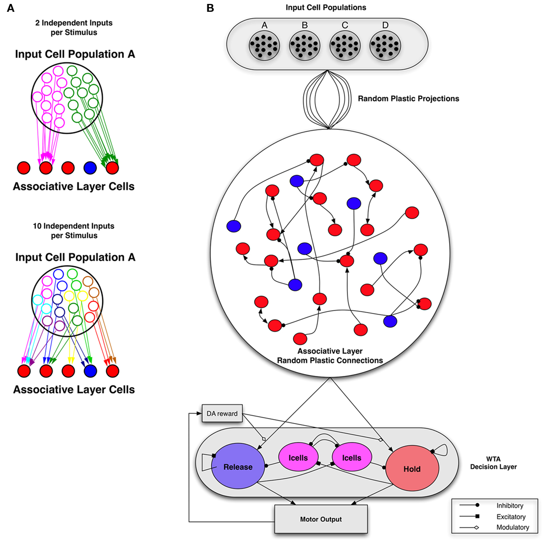
Figure 1. Network architecture. (A) Example of input configurations from a single stimulus-responsive input population. Each input population is represented by 20 cells, which output independent Poisson spike trains but correlated connections. The total number of independent sets of connections ranges from 2 to 20. Left: with two independent inputs per stimulus population, and low input connection probability (1/5 is shown) associative layer cells receive selective input. Right: with 10 independent inputs per stimulus population, and low input connection probability (1/5 is shown) associative layer cells receive more uniform, less correlated inputs. Poisson input groups randomly project to a sparse-random recurrent network of excitatory (red) and inhibitory (cells). Input projection probability ranges from 1/20 (sparse) to 1/2 (dense), with input connections selected independently between each set of independent input cells per input population. (B) Complete network structure (Bourjaily and Miller, 2011). Excitatory-to-excitatory connections (arrows) and inhibitory-to-excitatory connections (balls) are probabilistic and plastic. All-to-all inhibitory-to-inhibitory synapses are also present but not plastic. In the relevant simulations, STDP or triplet-STDP occurs at excitatory-to-excitatory and input-to-excitatory synapses, while LTPi occurs at inhibitory-to-excitatory synapses. Inhibition is feed forward only (i.e., the network does not include recurrent excitatory-to-inhibitory synapses). Excitatory cells from the Associative layer project all-to-all, with initially equal synaptic strength to excitatory cells in both the Hold and Release pools of the decision-making network. The decision-making network consists of two excitatory pools with strong intra-pool recurrent connections, which compete via cross-inhibition between pools (Wang, 2002). Strong intra-pool recurrent excitation ensures bistability for each pool, while the cross-inhibition generates winner-take-all (WTA) dynamics such that only one population can be active following the stimulus, resulting in one decision. Whether the motor output (based on the decision of hold versus release) is correct for the corresponding cue, determines the presence of Dopamine (DA) at the input synapses, according to the rules of the task in Figure 2.
The particular training protocol we used, biconditional discrimination (Figure 2A) is one that requires the network to produce an Exclusive-Or (XOR) logical response to pairs of activated stimuli (Dusek and Eichenbaum, 1998; Lober and Lachnit, 2002; Takeda et al., 2005; Sanderson et al., 2006; Harris et al., 2008, 2009). Production of XOR responses is non-trivial, since a correct set of responses cannot be achieved by making a choice according to a linear combination of the inputs (i.e., the task is not linearly separable; Hasselmo and Cekic, 1996; Senn and Fusi, 2005). Others have produced solutions of XOR tasks with neuronal networks via a variety of forms of reinforcement learning (Seung, 2003; Xie and Seung, 2004; Florian, 2007) or non-linear neural response (Hasselmo and Cekic, 1996; Christodoulou and Cleanthous, 2011). We find that our network achieves XOR-logic by enhancing initial selectivity of cells responsive to particular pairs of stimuli (Bourjaily and Miller, 2011; Christodoulou and Cleanthous, 2011). Generating selectivity to specific combinations of stimuli is a well-known function of sensory areas (Desimone et al., 1984; Ito et al., 1995; Baker et al., 2002). When coupled with a method for producing invariance, such stimulus-combination selectivity provides a framework for general feature and item detection (Serre et al., 2007). Thus, the task and ensuing XOR response simulated in our model networks is likely to be representative of many of the computations carried out by circuits of neurons throughout the brain.
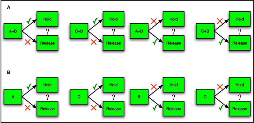
Figure 2. Task logic. (A) In an example of biconditional discrimination (Sanderson et al., 2006), two of four possible stimuli (A, B, C, and D) are presented simultaneously to a subject. If either both A and B are present or neither is present, the subject should make one response (such as release a lever). If either A or B but not both are present, the subject should make an alternative response (such as hold the lever until the end of the trial). Neurons must generate responses to specific stimulus-pairs (e.g., A + B) to perform this task successfully. A response to a single stimulus (e.g., A) is not sufficient to drive the correct response in one pairing without activating the incorrect response for the opposite pairing of that stimulus. (B) In the simplified task of single stimulus-response matching, network input is more specific, with just one input activated at a time.
We show that other stimulation protocols, with either more specific input and completely non-specific input (spontaneous background activity), can also lead to the structural correlations observed in vitro (Song et al., 2005; Perin et al., 2011), so long as the activity of cells is sufficiently diverse. We note that such heterogeneity across cells is necessary for producing solutions to the XOR-like behavioral task (Rigotti et al., 2010; Bourjaily and Miller, 2011).
The overall network structure and training protocols described below follow those from a previously published study (Bourjaily and Miller, 2011). Table 1 provides a summary of the model’s structure and parameters, in a form suggested for neuronal network models (Nordlie et al., 2009). In this paper we add structural plasticity to the networks studied previously and analyze the resulting changes in network structure in a manner similar to that used by Song et al. (2005) for the connections within cortical slice data.
Pairs of stimuli activated together (either A + B, C + D, A + D, C + B) produced inputs as Poisson spike trains. In order to investigate the robustness of each learning rule, we examined their effects on sets of 25 different networks with each set of networks explored under four or more distinct plasticity protocols.
We produced networks with different degrees of input correlations, as shown in Figure 1A, by altering the number of independent inputs per stimulus, as 2, 4, 6, 10, or 20 (6 in the default network) to excitatory and inhibitory cells in the associative layer (Figure 1B). Each input comprised a train of independent Poisson spikes with a mean firing rate defined by:  For example, in a network with 20 inputs any stimulus produced 20 independent Poisson spike trains at 24 Hz, with each input projecting to independent sets of cells within the associative layer. Whereas, with two inputs per stimulus, the two trains of 240 Hz Poisson spikes (a firing rate much higher than produced by an individual cell) can be considered as 20 independent Poisson spike trains of 24 Hz grouped into two sets of 10 – while the receiving cells between sets are uncorrelated, the receiving cells within such a set of 10 would be identical. Thus, as the number of inputs per stimulus decreases, the correlations in connectivity from afferent cells increases. In this paper we do not address structural plasticity of the input connections, which we expect to determine the actual level of input correlations.
We examined how the sparseness and correlations of input groups affected both the initial selectivity of a network and how the network responded to each of the synaptic plasticity rules. Input sparseness is defined via the probability of any input group projecting to any given cell. As input connection probability increases, sparseness decreases. We used the following five values for input connection probability: 1/2, 1/3, 1/5, 1/10, and 1/20 (1/5 in the default network).
Five levels of input sparseness, combined with 5 different degrees of input correlations led to 25 variant networks in each regime.
Our initial network possessed neither structure in its afferent connections nor in its internal recurrent connections. Random connectivity produced cell-to-cell variability since no two cells receive identical inputs. Such heterogeneity of the inputs across cells led to a network of neurons with diverse stimulus responses.
In a subset of examples (Figures 10 and 11A,C) we trained the network, with a single stimulus at a time (e.g., “A” alone) rather than with paired inputs (e.g., “A + B”; see Figure 2B). Total time of inputs was unchanged, but neural responses were sparser, producing greater selectivity (fewer cells active at any one time and any cell is active to fewer inputs).
We use leaky integrate-and-fire (LIF) neurons (Tuckwell, 1988) defined by the leak conductance, gL, synaptic conductances gAMPA, gNMDA, gGABA, and a refractory conductance, gref, resting potential (i.e., leak potential) VL and threshold potential, Vth. The threshold potential is dynamic: it increases to a maximal value of 150 mV immediately after a spike and decreases exponentially (with time constant 2 ms) to a cell-dependent base value (given below) between spikes. The membrane potential, V, evolves according to the equation:

reversal potentials for excitatory and inhibitory currents respectively. Rather than a hard reset, following a spike, we mimic delayed rectifier potassium currents with reversal potential, Vref = −70 mV, via a refractory conductance, gref, which increases immediately following a spike by δgref = 150 μS and decays to zero exponentially with a cell-dependent time constant, τref.
We model noise as independent excitatory and inhibitory synaptic conductance variables, drawn from a uniform distribution [0 gnoise] with gnoise = 1.2 mS/s1/2 in the associative layer cells in default networks and gnoise = 4 mS/s1/2 in the decision layer cells. In networks without stimuli, we increase the noise level (gnoise = 2.5 mS/s1/2) to produce sufficient levels of spontaneous activity for synaptic potentiation between some cells.
LIF neurons had a mean leak reversal potential of VL = −67.5 ± 1.25 mV, membrane time constant of τm = 10 ± 0.75 ms and leak conductance of gL = 36 ± 0.5 μS (see Table 2). Excitatory neurons had a firing threshold of Vth = −48 ± 1 mV, with time constant τth = 2.25 ± 0.125 ms a reset voltage of Vreset = −58 ± 1 mV, and a refractory time constant of τref = 2.25 ± 0.125 ms. Inhibitory neurons had a firing threshold of Vth = −48 ± 1 mV, a reset voltage of Vref = −58 ± 1 mV, and a refractory time constant of τref = 1.25 ± 0.125 ms. Heterogeneity of these parameters was drawn from uniform distributions with the given ranges.
Excitatory LIF neurons had a leak reversal potential of VL = −70 mV, membrane time constant of τm = 20 ms, and leak conductance of gL = 35 μS (see Table 2). Excitatory neurons had a firing threshold of Vth = −48 mV, a reset voltage of Vreset = −55 mV, and a refractory time constant of τref = 2 ms. Inhibitory LIF neurons had a leak reversal potential of VL = −70 mV, membrane time constant of τm = 10 ms, and leak conductance of gL = 30 μS. Inhibitory neurons had a firing threshold of Vth = −50 mV, a reset voltage of Vreset = −55 mV, and a refractory time constant of τref = 1 ms.
Synaptic currents were modeled by instantaneous steps after a spike followed by an exponential decay described by the equation (Dayan and Abbott, 2001) ds(t)/dt = −s/τs + Σk δ(t − tk). Recurrent excitatory currents with reversal potentials, VE = 0 mV, were modeled as mediated by AMPA receptors (τAMPA = 2 ms) and NMDA receptors (τNMDA = 100 ms). Inhibitory currents with reversal potential, VI = −70 mV, were modeled as mediated by GABAA receptors (τGABA = 10 ms). Conductance of NMDA receptors was modified by the voltage term FNMDA(V) (Jahr and Stevens, 1990):  with the external magnesium concentration,
  To assess whether this established voltage-dependence of NMDA receptors played any role in our network, we also ran simulations with the function set as a static value of FNMDA(V = −0.055).
Excitatory-to-excitatory connections are sparse with 10% connection probability. Initially connections are random and uncorrelated. Inhibition is feedforward only, so there are no excitatory-to-inhibitory connections. Inhibitory-to-Inhibitory connections are all-to-all. Finally, Inhibitory-to-excitatory synapses connect randomly with a probability of 25%. Initial excitatory-to-excitatory synaptic strength is taken from a uniform distribution, with a mean value of W0 = 0.05 and range of ±50% about the mean. These simulations were carried out in a network with 320 excitatory and 80 inhibitory neurons in our default implementation and all networks with increased size maintained the 4:1 excitatory:inhibitory ratio (Abeles, 1991). Connections to the decision layer are initially all-to-all from excitatory neurons with a uniform strength of DW0 = 0.075.
The decision-making network based on prior models (Wang, 2002) is composed of two excitatory pools (each containing 200 cells) and two inhibitory pools (each containing 50 cells. Excitatory-to-excitatory synaptic strength is W0 = 0.25. Connections within each pool are all-to-all. Cross-inhibition is direct from each inhibitory pool to the opposing excitatory pool, which generates winner-take-all activity so that only one pool is stable in the up state (active). Network bistability is generated by strong inhibition and self-excitation.
The decision-making network receives a linear ramping input that initiates at the start of the cue and continues until the end of the cue where it reaches its maximal value of gurgency = 5 μS at the end of the cue. This input is adapted from the “urgency-gating” model (Cisek et al., 2009), in order to ensure that a decision is made each trial.
For all connections undergoing functional plasticity, changes in synaptic strength are limited to a maximum of 50% per trial (the maximum potentiation seen in typical experimental protocols) while across all trials, synaptic strength is bounded between 0 and 10 times W0, the initial mean synaptic strength.
Long-term potentiation of inhibition (LTPi) is modeled after (Maffei et al., 2006): LTPi occurs when an inhibitory cell fires, but the post-synaptic excitatory cell is depolarized and silent. If the excitatory cell is coactive (i.e., spiking), then there is no change in the synapse strength. We refer to this as a veto effect in our model of LTPi. Any excitatory spike within a window of ±20 ms for an inhibitory spike will result in a veto. For each inhibitory spike (non-vetoed) the synapse is potentiated by idW = 0.001. LTPi was reported experimentally as a mechanism for increasing (but not decreasing) the strength of inhibitory synapses in cortex (Maffei et al., 2006). To compensate for the inability of LTPi to depress synapses, we use multiplicative post-synaptic scaling (Turrigiano et al., 1998b) for homeostasis at the inhibitory-to-excitatory synapses. We explicitly model the post-synaptic depolarization required by LTPi by defining a voltage threshold that the post-synaptic excitatory cell must be above in order for potentiation to occur. We used a value of −65 mV, which is 5 mV above the leak reversal. Finally, we include a hard upper bound of inhibitory synaptic strength, such that those cells most strongly inhibited (so being less depolarized as well as not spiking) in practice receive no further potentiation of their inhibitory synapses.
We implement basic STDP according to standard methods (Song et al., 2000) assuming asymmetric exponential windows for potentiation when a presynaptic spike at time tpre precedes a post-synaptic spike at time tpost, and for depression if the order is reversed. Thus the change in connection strength, ΔW, follows:

and

All pairs of presynaptic with post-synaptic spikes are included (i.e., all-to-all). Basic STDP produces changes in synaptic weight whose sign depends only on the relative order of spikes, thus only on the relative order and direction of changes in rate, not on the absolute value of the rate. The LTD amplitude A− was 0.80, and the LTP amplitude A+ was 1.20. The LTD time constant, τ−, was 25 ms; the LTP time constant, τ+, was 16 ms.
Triplet-STDP was modeled after the rule published by Pfister and Gerstner (2006). Their model includes triplet terms, so that recent post-synaptic spikes boost the amount of potentiation during a “pre-before-post” pairing, while recent presynaptic spikes boost the amount of depression during a “post-before-pre” pairing.
Specifically if tpost − tpre > 0,

while if tpost − tpre < 0,

We use the parameters cited from the full model “all-to-all” cortical parameter sets in the paper (Pfister and Gerstner, 2006). The amplitude terms are doublet LTP  doublet LTD
  triplet LTP
  and triplet LTD
  The time constants we used are τ+ = 16.68, τ− = 33.7, τy = 125, and τx = 101 ms. These parameters generated an LTD-to-LTP threshold for the post-synaptic cell of 20 Hz, above which uncorrelated Poisson spike trains produce potentiation and below which they produce depression.
Synapse stability is maintained by a homeostatic form of multiplicative post-synaptic scaling (Turrigiano et al., 1998b; Turrigiano and Nelson, 2000; Renart et al., 2003) with synaptic strengths updated on a trial-by-trial basis as  where the mean rate of the post-synaptic cell, j, is
  and its goal rate is
  We use the parameter ε = 0.001 for all synapses. Goal rates for all types of cell and synapse were taken from a uniform distribution, with mean 8 Hz and range ±50%. Others have shown the value of homeostatic rules for stabilizing networks with otherwise unstable STDP (Kempter et al., 2001). Our implementation (Renart et al., 2003; Bourjaily and Miller, 2011) results in the strengthening of synapses even in the absence of any post-synaptic spikes, as seen in cortical slices (Turrigiano et al., 1998a), so in this sense it is related to homeostatic rules that normalize (Lazar et al., 2009) or otherwise constrain total synaptic input onto a cell (Fiete et al., 2010), rather than those which shift the parameters for STDP (Bienenstock et al., 1982; Clopath et al., 2010) or produce homeostasis via the inherent structure of the STDP window (Kempter et al., 2001).
Synapses to the decision-making layer from the associative layer are modulated according to a dopamine-based reward-prediction error signal (Soltani and Wang, 2006, 2010; Soltani et al., 2006), which in essence produces Hebbian learning when unanticipated reward arrives, and anti-Hebbian if delivery of reward does not meet expectations (Schultz, 1998, 2010; Reynolds et al., 2001; Reynolds and Wickens, 2002; Jay, 2003; Shen et al., 2008; Fremaux et al., 2010).
Excitatory synapses onto decision-making cells that belong to the “winning” population, as defined by a mean firing rate above rwin = 25 Hz following the end of stimulus presentation, are modified by an amount proportional to the square of the mean presynaptic firing rate multiplied by the reward-expectation error.
The reward-expectation is calculated from a geometrically weighted sum of the 5 prior rewards to that stimulus-pair, such that each trial contributes +1 when rewarded, −1 if not rewarded, with a weight that decreases by a factor of 0.5 for successive trials in the past. The reasoning is that once the behavior predictably produces reward, the reward-expectation error becomes zero and no dopamine signal arises upon reward delivery. For the network, once the response produces reward reliably, the reward-expectation reaches one, so delivery of reward produces no further plasticity in synapses to the decision-making layer. Results in studies without this factor (by setting reward-expectation to zero on all trials) were similar (Bourjaily and Miller, 2011).
Our rule for structural plasticity assumes that synapses disappear if there is little Hebbian-like causal correlation between presynaptic and post-synaptic spikes, which could be detected by a calcium signal (Helias et al., 2008). The synapses are replaced at random to maintain the total number of connections at a constant value. We consider three types of random replacement:
(1) Select at random a new presynaptic cell, keeping the same post-synaptic cell.
(2) Keep the same presynaptic cell, but select at random a new post-synaptic cell.
(3) A 50% choice of process (1) or process (2).
The criterion for selection of synapses to be removed is based on three parameters:
(1) The width of a temporal window for coincidence of spiking – if a post-synaptic cell spikes within such a temporal window following a presynaptic spike, the synapse between the two cells is more likely to be retained.
(2) The frequency of such coincidences necessary to prevent removal of the synapses.
(3) The number of trials without sufficient numbers of coincident spikes to result in removal of the synapse.
The main effect of changing these parameters is to alter the number of synapses that get removed across trials, rather than changing from removal of one set of synapses to another set. Thus, the magnitudes of correlations are affected by parameter changes, but not the overall sign and directions of correlations.
The specific implementation of structural plasticity under our default parameter set is to update a parameter, Sij, for each synapse between presynaptic cell i and post-synaptic cell j following each trial, and remove the synapse if Sij falls below a threshold, τ = −8. Any new synapse and all synapses at the beginning of the simulation are initialized with Sij = 0. Within a trial, for each pair of presynaptic and post-synaptic spikes at times ti and tj respectively, with tj > ti, we increase Sij according to: Sij |→ Sij+exp[−(tj − ti)/τStruc], where τStruc = 25 ms. The necessary rate of coincident spiking to prevent loss of a synapse is given by the value R = 1, which is subtracted from Sij after each trial: Sij |→ Sij − R. Thus a new synapse can be removed after 8 trials (because − T/R = 8) if its presynaptic and post-synaptic neurons produce no causally coincident spikes in these trials. The more coincident spikes in the past history of the synapse, the more trials it can survive without coincident spiking, thus strong synapses are more stable. In our simulations, since the total numbers of inputs are the same for every block of four trials, the history-dependence is not an important factor (we set an upper bound on Sij of  but either increasing or decreasing this by a factor of two, or even removing the bound has no significant effect – see Table A1 in Appendix).
As a control, we produced a network of 320 excitatory cells, randomly assigning each cell to one of four assemblies. We then assigned synaptic connections randomly, but with connection probability within an assembly, PS = 0.2 or 0.35, higher than the mean connection probability, 〈P〉 = 0.1 and therefore higher than the mean connection probability between assemblies, PX = (4〈P〉 − PS)/3. Connection strengths were selected randomly from a Gaussian distribution with mean of 2, SD 0.5 for within-assembly connections, and with a mean of 1, SD 0.25 for between-assembly connections (negative values were reselected). We did not simulate the activity of such a network, but assessed how the correlations among connections produced in such a simple manner match the observed data.
Simulations were run for either 400 trials or 2000 trials as stated – in most networks a steady state was achieved (Carnell, 2009) by 1000 trials – using the Euler-Maruyama method of numerical integration with a time step, dt = 0.02 ms. All simulations were run across at least four random instantiations of network structure, cell and synapse heterogeneity, and background noise. Simulations were written in C++ on Intel Xeon machines. Matlab R2010a was used for data analysis and visualization.
Stimulus-pair selectivity,  defines for each excitatory neuron, i, its selectivity for one stimulus-pair over the other three stimulus-pairs.
  is the maximum firing rate of neuron i, minus its mean response across all stimuli, normalized by its mean response:
  The network’s stimulus-pair selectivity value, 〈SPS〉 is the mean of
  taken across all excitatory cells. The measure ranges from 0 to 3 and was found to correlate better with performance on the paired-stimulus task than a similar metric without weight normalization (Bourjaily and Miller, 2011). Cells are only included if their mean rate is greater than 1 Hz to at least one stimulus-pair.
We calculated three different indices to represent the amount of clustering in the network. The bidirectional ratio, σbi, is the ratio of number of pairs of cells with bidirectional connections divided by the number expected by chance: σbi = Nbi/〈Nbi〉 where 〈Nbi〉 = pactNconns/2 ∼ p2Ncells(Ncells − 1)/2 with p the given connection probability (p = 0.1 in our default networks) and pact is the actual connection probability (the approximate instantiation of p), pact = Nconns/[Ncells(Ncells − 1)]. Ncells is the total number of excitatory cells (Ncells = 320 in our default networks) and Nconns is the total number of connections in that instantiation of the network (Nconns is typically slightly different from its expected number, 〈Nconns〉 = pNcells(Ncells − 1), because initial connections are chosen probabilistically). The triplet ratio is the number of fully connected triplets of cells (motifs numbered 10–16 in Figure 4A) divided by the expected number: σtri = Ntri/〈Ntri〉 where  in which plink is the probability of any connection (whether unidirectional or bidirectional) between two cells: plink = 1 − (1 − pact)2. The clustering coefficient of a network is defined as the number of triplets that are fully connected (all pairs in the triplet share a link) divided by the number of triplets that are at least partially connected (all cells are connected to at least one other in the triplet). In terms of our motifs in Figure 4A, the clustering coefficient is the sum of numbers of motifs numbered 10–16 divided by the sum of motifs numbered 4–16. For a network with connection probability, p = 0.1, so plink = 0.19 and the clustering coefficient for a random network is
We compare the number of each triplet motif (labeled 1–16, Figure 4A) with the expected number calculated using the numbers of pairs of cells found to be unconnected (with probability pno) or unidirectionally connected (with probability puni, thus puni/2 for a given direction) or bidirectionally connected (with probability pbi) and assuming these probabilities are uncorrelated across pairs as a random control. Hence the expected number〈Ni〉 of any triplet motif labeled i is given by:  where n0(t), n1(t), and n2(t) are respectively the number of pairs in the triplet motif with 0, 1, or 2 connections, such that n0(t) + n1(t) + n2(t) = 3 ∀ i and Ci is a combinatorial factor which takes into account the number of ways a triplet of cells can form the same motif, as given in Table 3.
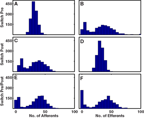
Figure 3. Histograms of numbers of outgoing and incoming intra-network connections per cell for different structural plasticity mechanisms. (A,B) Switching presynaptic cell. (C,D) Switching post-synaptic cell. (E,F) Select with 50% probability either presynaptic cell or post-synaptic cell to be switched. In all cases, network with 6 input groups per stimulus, 1/20 input connection probability and undergoing combined triplet-STDP with LTPi.
For the majority of comparisons of plasticity mechanisms, for each of the 25 separate input configurations to an associative layer network (Figures 1A,B), we produced four instantiations of the associative layer network itself and performed paired t-tests across individual input configurations, reporting a significant difference in an individual configuration if p < 0.002 (5% significance with Bonferroni correction) as well as a paired t-test for a global effect across all 100 networks. For certain controls (stated as one-network comparison) we tested just one version of the associative layer network with 25 different input configurations and performed a paired t-test versus the same 25 examples of the control networks and a two-sample t-test between the four control versions of the network and the version with altered parameters for each individual configuration.
When analyzing triplet motifs, we also calculate a Z-score (Zi) from the numbers of each motif, i, expected for a random network as Zi = (Ni − 〈Ni〉)/Σi where Ni is the number of a given motif in the network, and 〈Ni〉 = piN(N − 1)(N − 2)/6 is the expected number for a random network, where pi is the probability of any given triplet containing that motif (as described by the calculation in the previous section). We approximate Σi by assuming a Binomial distribution, such that 
Our formulations of structural plasticity are Hebbian, requiring a presynaptic spike to precede a post-synaptic spike sufficiently often to prevent synapse removal. Since we assume that cells have no mechanism to detect correlations in their activity until a connection forms, new connections are selected at random, via three different methods. In the first method, once a synapse is removed, we provide the post-synaptic cell with a new, randomly chosen afferent connection. This method is analogous to keeping the number of dendritic spines constant but allowing spine mobility to produce new connections. Thus, the number of incoming, afferent connections per cell remains constant while the number of outgoing, efferent connections can vary greatly across the network (Figures 3A,B). The second method is a mirror of the first, as we provide the presynaptic cell with a new, randomly chosen, post-synaptic partner. This is analogous to maintaining the number of axonal boutons per cell, but allowing them to move and connect to new cells. Thus the number of efferent connections does not change, but a broad distribution of numbers of afferent connections arises (Figures 3C,D). In the third method, neither number of afferents nor efferents is fixed (Figures 3E,F) as with equal probability we either randomly select a new presynaptic cell or randomly select a new post-synaptic cell. Indeed, the latter method produces a highly significant correlation (Σ = 0.97, p < 10−100) between the number of afferent and efferent partners of each cell. Such a correlation arises, as fewer inputs lead to fewer spikes by a cell, and fewer spikes by the cell mean fewer coincidences of spikes with those of post-synaptic partners – and such coincidences are necessary to retain a synapse. All of these methods assume processes arising from one cell move to form a new partner. The other logical possibility of choosing a totally new random pair of cells, is less biological, and produces results qualitatively matching our third method (data not shown). We note that following structural plasticity, some cells may lack efferents or afferents or both, depending on implementation. Such a result is not unreasonable when considering the relatively small number of excitatory cells (320) and the paucity of activated stimuli that are simulated.
All three implementations of structural plasticity produced similar changes in the numbers of bidirectional connections, but produced differences in the patterns of connections (motifs numbered 1–16 in Figure 4A) among triplets of cells (Figure 4). The most obvious difference between switching presynaptic versus switching post-synaptic cells in the structural plasticity rule appeared in the motifs numbered 4 and 5 of Figure 4A. If the presynaptic cell was switched, so that some cells had more efferent projections than others then motif 4 arose more often (Figures 4B,E) whereas if the post-synaptic cell was switched all cells had the same number of efferent projects but some received more connections and motif 5 was more common (Figures 4C,F). In vitro data (Song et al., 2005) demonstrate an excess of motif 4. Our third implementation (Figures 4D,G) produced an excess of motif 4, but also an excess of motif 11 – and all other connected triplets, motifs 10 and higher – in agreement with in vitro data (and unlike the first two methods). Thus, for optimal agreement with in vitro data (Song et al., 2005) we use the third implementation as our default method for the rest of this work.
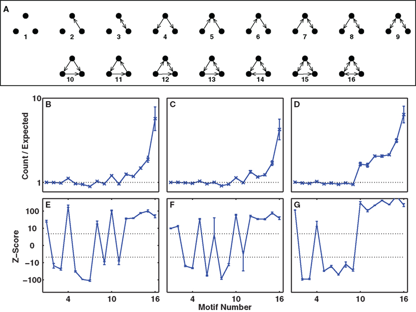
Figure 4. Overrepresentation of specific three-cell motifs. (A) List of motifs representing the possible connectivity patterns of three cells (Song et al., 2005). Motifs numbered 10 or higher are connected triplets that contribute to the clustering coefficient and triplet ratio. (B–D) Ratio of numbers of motifs produced to numbers expected by chance, given the unidirectional and bidirectional connection probabilities. (E–G) Z-scores for the numbers of motifs plotted on a non-linear (cube-root) scale. Dashed-lines represent p = 0.001, Z = ±3.3. (B,E) Switching presynaptic cell produces excess of motif 4, deficit of motif 5. (C,F) Switching post-synaptic cell produces deficit of motif 4, excess of motif 5. (D,G) Select with 50% probability either presynaptic cell or post-synaptic cell to be switched produces excess of motif 4, deficit of motif 5. Results are for our default network (6 independent inputs per stimulus, with input connection probability 1/20, trained for 2000 trials with LTPi and triplet-STDP).
Initially, internal connections were random (with 10% probability), so numbers of bidirectional connections or connected triplets of cells were at chance level. In all simulations we included structural plasticity, but varied the types and combinations of functional plasticity, including cases with structural plasticity alone if we omitted functional plasticity. Following 2000 trials of training our default network in biconditional discrimination (Figure 2A) while undergoing both LTPi and triplet-STDP (Pfister and Gerstner, 2006) with homeostasis, the ratio of number of pairs with bidirectional connections to the expected number by chance increased to 5.4 ± 0.1 (four independent simulations). The numbers of fully connected triplets (motifs 10 or higher, Figure 4A) similarly increased, by a factor, 5.9 ± 0.2 relative to chance. If, while retaining structural plasticity and triplet-STDP, we did not include LTPi, so that inhibition to excitatory cells remained unchanged from their initial value, then the ratios were smaller, namely 4.2 ± 0.2 for connected doublets and 5.2 ± 0.2 for fully connected triplets. Moreover, the ratios for networks with LTPi but no triplet-STDP were 3.5 ± 0.2 for doublets and 3.9 ± 0.3 for triplets, showing that inhibitory plasticity allowed structural plasticity to sculpt excitatory connections to a similar extent as a Hebbian form of excitatory plasticity. In fact, with neither triplet-STDP nor LTPi, changes produced by structural plasticity alone led to ratios of 1.77 ± 0.03 for connected doublets and 1.96 ± 0.04 for connected triplets. These results are summarized in Table 4.
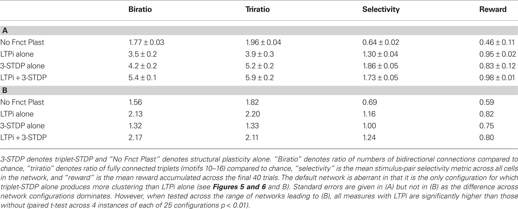
Table 4. Structural indices, selectivity and performance of the default network (A) and the mean of 25 configurations (B).
To assess the generality of our result, for each combination of plasticity mechanisms, we produced 25 types of network, differing in their input structure via 5 values of connection probability per input (1/20 to 1/2) and 5 values for the number of different random sets of input connections activated per stimulus (2–20; see Network Inputs). Figure 5 demonstrates that addition of LTPi during training with structural plasticity (C compared to A; D compared to B) increased the number of pairs of neurons with bidirectional connections. Moreover, in this type of protocol with paired stimuli, we found that triplet-STDP often reduced the number of such pairs (B compared to A; D compared to C). Indeed, our default network (chosen because it produced the most clustering) was the only one where triplet-STDP alone produced more bidirectional connections than LTPi alone. Across input configurations each of the two protocols with LTPi produced more bidirectional connections than each of the two protocols without LTPi (paired t-test, 4 instantiations per configuration, p < 0.01 versus structural plasticity alone, p < 10−4 versus triplet-STDP; see Figure 5).
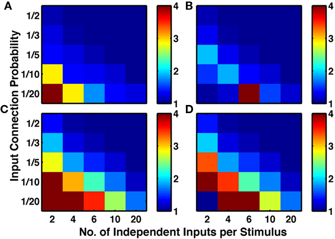
Figure 5. Inhibitory plasticity boosts numbers of bidirectional connections between excitatory cells. Sets of five by five networks with different degrees of sparseness of inputs (y-axis where low input probability reflects high sparseness of inputs) and different degrees of input correlations (x-axis where more input groups per stimulus reflects lower correlations). (A) Network with structural plasticity alone. (B) Network with triplet-STDP and structural plasticity. (C) Network with LTPi and structural plasticity. (D) Network with triplet-STDP, LTPi, and structural plasticity. In both cases (A–C) and (B–D), the addition of inhibitory plasticity increases the numbers of networks with excess bidirectional connections (color bar, red = 4 times chance, blue = chance). Networks trained for 2000 trials of the biconditional discrimination task.
These results, showing an increase in ratio by LTPi and often a decrease in ratio by triplet-STDP, were reproduced when analyzing the excess of fully connected triplets (Figure 6), indicative of a high clustering coefficient.
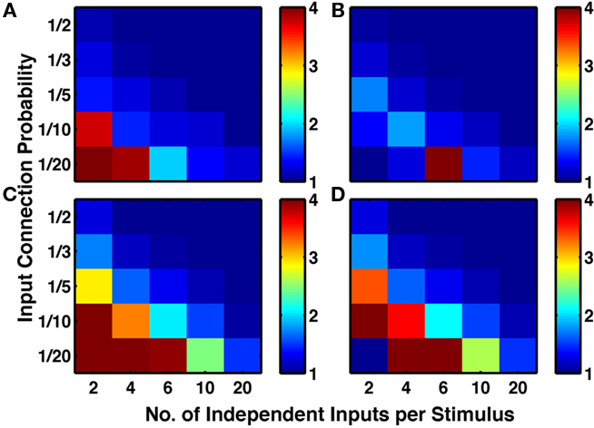
Figure 6. Inhibitory plasticity boosts numbers of connected triplets of excitatory cells. Sets of five by five networks with different degrees of sparseness of inputs (y-axis where low input probability reflects high sparseness of inputs) and different degrees of input correlations (x-axis where more input groups per stimulus reflects lower correlations). (A) Network with structural plasticity alone. (B) Network with triplet-STDP and structural plasticity. (C) Network with LTPi and structural plasticity. (D) Network with triplet-STDP, LTPi, and structural plasticity. In both cases (A) versus (C) and (B) versus (D), the addition of inhibitory plasticity increases the numbers of networks with excess connected triplets (color bar, red = 4 times chance, blue = chance). Networks trained for 2000 trials of the biconditional discrimination task.
In a prior publication (Bourjaily and Miller, 2011) we showed the necessity of high stimulus-pair selectivity among cells in the associative network (Figure 1B) to produce reliably correct behavior as determined by the trained output of a biologically inspired decision-making network (Wang, 2002). Moreover, in many of these networks, LTPi was necessary to produce the requisite high stimulus-pair selectivity. LTPi enhanced cross-inhibition, as inhibitory cells selective to a stimulus would strengthen their inhibitory connections preferentially to excitatory cells with low activity. Such an enhancement of cross-inhibition led to an increase in stimulus selectivity, as excitatory cells would receive less inhibition for their preferred response. Increased stimulus selectivity of cells would increase correlations in firing rate between cells, as the activity of cells became grouped by their preferred stimulus. Structural plasticity would then increase the connection probabilities between coactive cells (Figure 8). Thus, in our protocol, LTPi led to more clustered connections among cells, because such clustering of connections arises when subsets of cells are active strongly together for a small subset of stimuli – a feature of cell assemblies. Such behavior was indicated by a high stimulus-pair selectivity index for the network, and correlated with reliable decision-making and high accumulation of reward in the task, even without structural plasticity. If the production of cell assemblies by structural plasticity relies on the same correlations in activity that produce stimulus selectivity and reliable performance in our task, then one expects to see correlations between measures of clustering and measures of network performance.
Indeed, Figure 7 (blue crosses) demonstrates, across 100 different networks (4 random instantiations of each of 25 types) the high correlation between either paired-stimulus selectivity (Figures 7A,B) or accumulated reward (Figures 7C,D) and either the excess of bidirectional connections (Figures 7A,C) or fully connected triplets of cells (Figures 7B,D) in networks trained with LTPi and triplet-STDP combined with homeostasis and structural plasticity. Similar results hold for networks trained with LTPi alone (Figure 7, red circles) or triplet-STDP alone (green plus signs) when combined with homeostasis and structural plasticity.
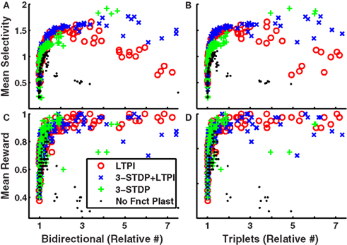
Figure 7. Excess of bidirectional connections and connected triplet motifs is highly correlated with biconditional discrimination task performance across networks. (A–D) Each data point represents results for a single network. 4 instantiations of each of 25 configurations with each plasticity mechanism: LTPi alone, red circles; LTPi with triplet-STDP, blue crosses; triplet-STDP alone, green plus signs; no functional plasticity, black dots. All networks incorporate homeostasis and structural plasticity. Networks with high stimulus selectivity (averaged over cell responses) produce (A) excess bidirectional connections and (B) excess connected triplets. The average reward per trial, is highly correlated with numbers of (C) bidirectional connections and (D) connected triplets (see Table 5). Networks trained for 2000 trials of the biconditional discrimination task.
Figures 7A,B suggest a threshold value of stimulus-pair selectivity (approximately 1.2), above which the neural firing is sufficiently structured to produce the high clustering of connections. Since reward accumulation also relies on selective responses, we find all of these features are significantly correlated with each other as shown in Table 5. However, networks with structural plasticity alone (no functional plasticity; Figure 7, black dots) showed the opposite correlation. Upon further examination, we find that in networks without triplet-STDP (i.e., those with structural plasticity combined with LTPi alone or no functional plasticity) performance and stimulus-pair selectivity are strongly positively correlated with clustering for low levels of clustering (ratios below 1.5). However, under these plasticity conditions, the highest degree of clustering is produced within the sparsest networks, with few independent inputs per stimulus, which have poor stimulus-pair selectivity and low reward accumulation. These networks contain isolated, strongly interconnected cell groups that are responsive to single stimuli, but are not stimulus-pair-selective. Thus, in networks with sparse activity, such that cells respond to single stimuli alone, the stimulus-dependent correlations in firing rate can lead to high clustering, without the concomitant high stimulus-pair selectivity necessary for good task performance.
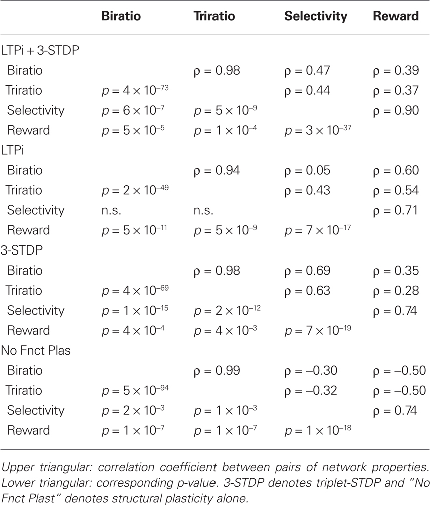
Table 5. Correlations among properties of trained networks with the four combinations of functional plasticity.
Networks trained with basic STDP and structural plasticity (data not shown) never exceeded chance performance in the task and produced minimal stimulus-pair selectivity (never exceeding 0.5 and typically below 0.1). However, some of these networks did produce an excess of bidirectional connections and high clustering compared to chance. Such clustering of connections arose between a subset of highly active, non-selective cells, while other cells became silent.
Figure 8 confirms (in our default network) that clustering is via increased connectivity between coactive cells. We labeled cells by their preferred stimulus-pair and separated the triplet motifs according to the three labels of the connected cells. We found that trios of cells with identical labels, meaning the cells were coactive to the same stimulus-pairs, dominated triplet motifs.
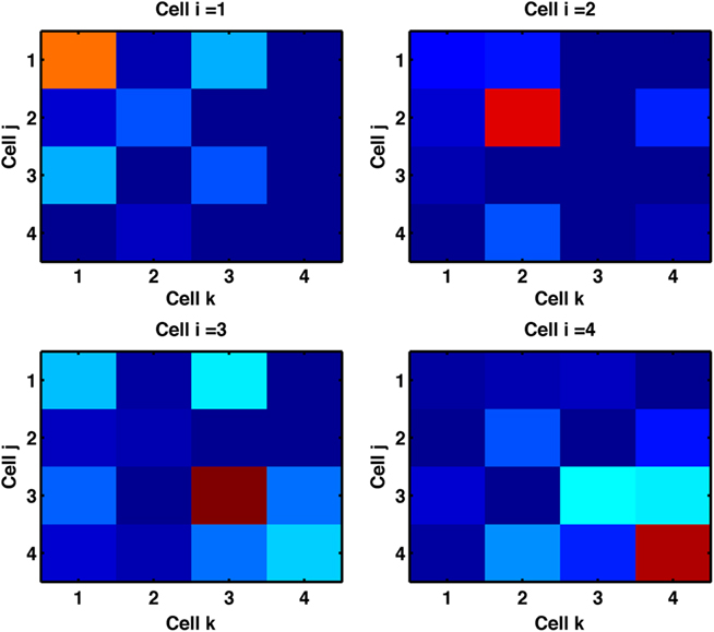
Figure 8. Cells with similar response properties cluster together. We label each cell by the stimulus-pair to which it is most responsive. For each of the three cells (indexed i, j, k) in fully, bidirectionally connected triplets (all examples of motif 16) we record the combinations of three most responsive stimuli. Color denotes the counts of these combinations across the network. The single highlighted squares on the diagonal indicate triplets of cells most responsive to the same stimuli are found fully connected. For example, the top-left panel shows that a cell most responsive to stimulus-pair A + B is predominantly found in triplets with both other cells most responsive to stimulus-pair A + B. Results are from the default network (input probability of 1/20 and 6 cell groups per input) trained with triplet-STDP and LTPi for 2000 trials of the biconditional discrimination task.
We assessed changes in synaptic strength of excitatory-to-excitatory connections, in our default network trained with a combination of triplet-STDP and LTPi with structural plasticity. Figure 9A indicates the non-Gaussian (though unimodal) distribution of connection strengths, with a long tail to higher strengths, as is observed experimentally (Song et al., 2005; Lefort et al., 2009). Nonetheless, the hard bound on synaptic strength of 0.5 (10 times initial strength) was rarely reached, even after 2000 trials by any synapses in these simulations.
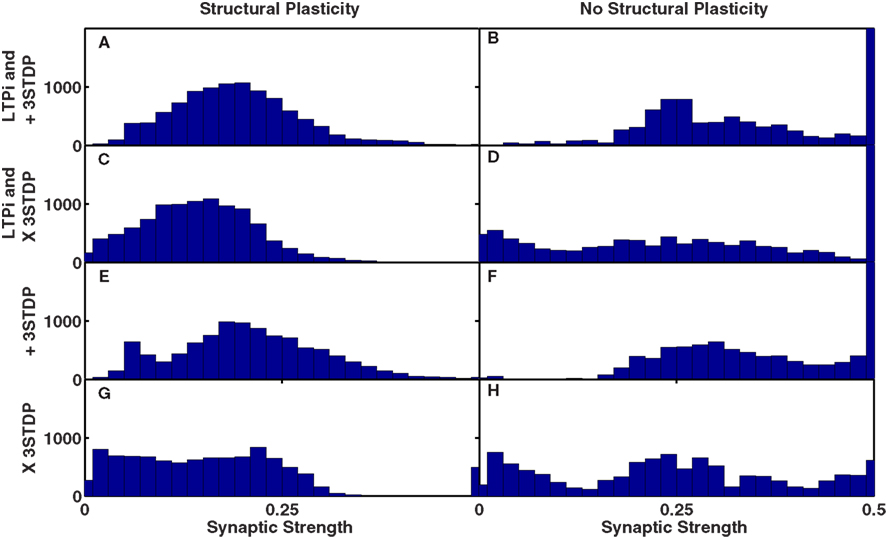
Figure 9. Unimodal distributions of synaptic strength produced by structural plasticity with homeostatic multiplicative synaptic scaling. In all networks, initial synaptic strength has a mean of W0 = 0.05 and maximum synaptic strength is Wmax = 0.5. (A–D) Functional plasticity is LTPi and triplet-STDP. (E–H) Functional plasticity is triplet-STDP alone. (A,C,E,G) (Left) Networks with structural plasticity included. (B,D,F,H) (Right) Networks without structural plasticity. (A,B,E,F) Triplet-STDP is the default additive rule (+3-STDP). (C,D,G,H) Triplet-STDP includes the multiplicative term (X STDP) that produces unimodality when analyzed for a single cell. Results are from the default network (input probability of 1/20 and 6 cell groups per input) trained for 2000 trials of the biconditional discrimination task. Note the initial distribution, and distribution of strengths of all replacement connections is uniform between 0.025 and 0.075.
Spike-timing-dependent plasticity rules that are additive (van Rossum et al., 2000) typically produce a bimodal distribution of synaptic strengths. Multiplicative STDP reproduces the experimentally observed unimodal distribution of synaptic weights of inputs to a single cell (van Rossum et al., 2000); thus we also trained networks with such a rule, whereby any increase in synaptic strength was multiplied by a factor: (Wmax − W)/Wmax − W0 where W, W0, and Wmax are respectively the current, the mean initial and the maximum values of synaptic strengths. In our simulations with structural plasticity, the distribution of weights (for all synapses in the network) was unimodal, even with additive triplet-STDP (Figures 9A,C). Moreover, when we removed structural plasticity, even with multiplicative triplet-STDP, we observed a bimodal distribution of synaptic strengths, with a large number of synapses reaching the maximum value (Figures 9D,H).
Analysis of our results indicates that the distribution of synaptic strengths was dominated by cell-to-cell variability (Koulakov et al., 2009) resulting in a striated, plaid-like structure of the connectivity matrix (see Figure A5 in Appendix). Without structural plasticity, the most active cells had the most strengthened input synapses, with the values readily reaching the upper bound, even though homeostasis by multiplicative synaptic scaling acted to oppose the trend. In the presence of structural plasticity, these cells gained more input synapses, so they could achieve the same firing rates (where homeostasis would compensate ongoing Hebbian synaptic strengthening) with a lower mean synaptic strength. Thus, the combination of structural plasticity with homeostasis via multiplicative scaling allowed the steady state synaptic strength of the most active neurons to be lower, preventing a pile up of synaptic strengths at the upper bound and the ensuing bimodality of the distribution.
In vitro data shows that bidirectional synapses are stronger than unidirectional ones (Song et al., 2005), a feature reproduced in a network model with a different protocol from ours (Clopath et al., 2010). In our default network (6 independent inputs with connection probability 1/20) the mean strength of bidirectional connections was significantly greater than that of unidirectional connections (p < 10−100, two-sample t-test) with a ratio of 1.2. A similar increase in strength of bidirectional connections was observed in other networks with a high degree of clustering if trained with triplet-STDP (with or without LTPi; see Figures A6B,D in Appendix). However in some networks we found stronger unidirectional connections. Such a reduction in the relative strength of bidirectional synapses is a consequence of homeostasis, and indeed was the norm in networks trained with LTPi alone, where homeostasis was the only mechanism to alter excitatory synaptic strength (Figure A6C in Appendix).
All networks with a significant excess of bidirectional connections produced a positive correlation in the strengths of reciprocal synapses when trained with additive triplet-STDP (Figure A5 in Appendix). Such a result may be expected from the rate-dependence of triplet-STDP and agrees with work using a voltage-dependent STDP mechanism (Clopath et al., 2010) and cortical slice data (Song et al., 2005). The rate-dependence of triplet-STDP causes a strengthening of connections in both directions between two cells if they are highly active at the same time. By contrast, basic STDP (unless dendritic delays are prominent; Lubenov and Siapas, 2008; Morrison et al., 2008) can only produce negative correlations between reciprocal connections, since any spike pair that increases the strength in one direction would reduce the strength in the reciprocal direction. Moreover, basic STDP alone can lead to a loss of connected loops (Kozloski and Cecchi, 2010) that are a necessary component of high clustering in networks.
By simplifying the protocol to be a single stimulus at a time (Figure 2B), we increased the stimulus specificity and the sparseness of neural firing. In these examples, the network is functioning only to relay in a noisy manner the information already present in the input groups, so is unlikely to be an ideal model of cortical activity. Nevertheless the simplified protocol highlights that once we had a network with different subsets of cells active at different times, our implementation of structural plasticity enhanced the amount of bidirectional connectivity (Figure 10). Indeed, since selective responses to single stimuli appeared in the majority of initial (i.e., untrained), randomly connected networks, structural plasticity alone was sufficient to produce the observed excess (Figure 10A).
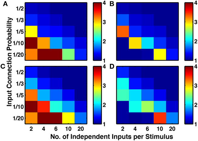
Figure 10. Stronger stimulus specificity produces networks with high numbers of bidirectional connections. If single stimuli are activated, rather than paired stimuli, more selective responses arise, with less need for functional plasticity. Sets of five by five networks with different degrees of sparseness of inputs (y-axis where low input probability reflects high sparseness of inputs) and different degrees of input correlations (x-axis where more input groups per stimulus reflects lower correlations). (A) Network with no functional plasticity, just structural plasticity. (B) Network with triplet-STDP and structural plasticity. (C) Network with LTPi and structural plasticity. (D) Network with triplet-STDP, LTPi, and structural plasticity. While in both cases (A–C) and (B–D) addition of inhibitory plasticity increases the numbers of networks with excess bidirectional connections, for many networks, structural plasticity alone is sufficient to produce excess bidirectional connections (color bar, red = 4 times chance, blue = chance). Networks trained with 400 trials of the single stimulus-response matching task.
Figures 11A,C indicated that the simplified protocol in our default network (2 input groups per stimulus with connection probability 1/5) readily reproduced the excess of connected triplets (motifs 10 or higher). All of the motifs for partially connected triplets of cells (motifs 2–9) were significantly less common than chance, in contrast to slice data (Song et al., 2005; Perin et al., 2011). It is likely that with the single stimulus protocol, cell responses are more correlated than in vivo so that partially connected triplets are more likely to become fully connected in this paradigm than in vivo.
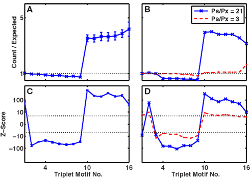
Figure 11. Triplets of connected cells appear with high stimulus specificity and in a cell-assembly network. (A,B) Ratio of numbers of three-cell connectivity motifs produced to numbers expected by chance, given the unidirectional and bidirectional connection probabilities. (C,D) Z-scores for the numbers of motifs plotted on a non-linear scale. Dashed-lines represent p = 0.001, Z = ±3.3. (A,C) Network with no functional, only structural plasticity, but highly selective responses via activation of single stimuli (after 400 trials). (B,D) Network designed as a set of four cell assemblies, with higher probability of connection, PS, within an assembly versus PX between assemblies. In both cases mean connection probability, 〈P〉 = 0.1, thus PX = (4〈P〉 − PS)/3. Solid blue line, with crosses, PS = 0.35; dashed red line with bullets, PS = 0.2.
Finally, we assessed how much of the slice data could be reproduced by a simple network of four cell assemblies (see Control Network of Cell Assemblies). With a mean connectivity probability maintained at 0.1 across all cells, when the within-assembly connection probability was increased to 0.2 (3 times greater than that between assemblies) we found an excess of bidirectional connections (p = 3 × 10−37, ratio to number expected was 1.4) and that bidirectional connections were on average stronger than unidirectional connections (p < 10−100, ratio was 1.37). Even though connections within a cell assembly were not correlated, because some bidirectional connections arose between assemblies – and in these cases both connections would be weak – the network produced a small but highly significant correlation in the strengths of the two synapses between pairs of cells with a bidirectional connection (ρ = 0.23, p = 2 × 10⁻⁹). The distribution of synaptic strengths was the sum of two overlapping Gaussians (one with mean 1, the other with mean 2, with SD of 0.25 and 0.5 respectively). Since the Gaussian with higher synaptic strength contained fewer total connections (only 1/4 of all cell pairs were within the same cell assembly, so only 1/2 of connections were strong and within a cell assembly) the overall shape of synaptic strength distribution had the same skew as the slice data (Song et al., 2005; Lefort et al., 2009). We found qualitatively similar, but quantitatively more pronounced results when we increased the within-assembly connection probability to 0.35 (becoming 21 times greater than that between assemblies).
Figures 11B,D indicates the patterns of connectivity among triplets of cells in these manufactured multiple-assembly networks. Although doubling the within-assembly connection probability to 0.2 (and reducing the between-assembly probability to 0.2/3) produced relatively small absolute changes in the numbers of triplet motifs compared to chance (red-dashed Figure 11B) nearly all patterns were still present at significantly greater than or significantly less than chance (outside the dotted lines denoting p = 0.001 in Figure 11D). In particular, the number of triplets with zero (motif 1), one (motif 2), or three (motifs 10–16) linked cells was greater than chance, whereas the number of triplets with only two of the three links present (motifs 4–9) was lower than chance. Increasing the within-assembly connection probability further to 0.35 (and reducing the between-assembly connection probability to 0.35/21) led to changes in the numbers of triplets more quantitatively similar to the experimental data (solid blue with crosses, Figures 11B,D). Thus, the only significant aspect of the slice data missing from the cell-assembly structure was the observed excess of motif 4 and dearth of motif 8 (Song et al., 2005).
In our default network, spontaneous activity was low, but when we raised the level of background noise within the associative layer, the rate of spiking activity can be sufficient to produce significant levels of functional and non-random structural plasticity in the absence of directed external input. Moreover, even in the absence of any functional plasticity or homeostasis, some networks with structural plasticity alone produced high degrees of clustering (Figure 12) based on the cell-to-cell variability in firing rate of a heterogeneous network. Indeed, when we rendered the cell parameters homogeneous, then structural plasticity produced no clustering, even when coupled with forms of functional plasticity (Figure 12). Thus, structural plasticity produced highly clustered groups of cells whenever large differences in concurrent levels of activity were present across cells. Such concurrent differences in firing rates arose within spontaneous activity when cells possessed sufficient heterogeneity. In such cases, coactive cells became highly connected with each other, as coincident spikes would maintain their synapses, whereas less active cells lost their connections, due to their dearth of coincident spikes with other cells.
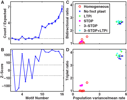
Figure 12. Clustering arises in random heterogeneous networks with raised spontaneous activity. (A,B) Excess of triplet motifs produced by structural plasticity in a default network with no functional plasticity and default, heterogeneous cells. (A) Ratio of counts for each motif (Figure 4A) to expected count. (B) Z-score (see Materials and Methods). (C) Ratio of bidirectional connections to expected number as a function of the variance of firing rates across cells of normalized by the population’s mean firing rate (Σ = 0.83, p = 1 × 10⁻⁴). (D) Ratio of numbers of triply connected motifs (numbered 10–16, Figure 4A) to expected number as a function of the variance of firing rates across cells of normalized by the population’s mean firing rate (Σ = 0.77, p = 8 × 10⁻⁴). (C,D) Networks labeled homogeneous had identical cells, but random connectivity, with variable base firing rates and plasticity mechanisms. Otherwise cells were heterogeneous (see Materials and Methods) with the indicated plasticity mechanisms. Results are based on all 320 excitatory, associative layer cells in a default network with no inputs, but with increased AMPA and GABA conductance noise (gnoise = 2.5 mS/s1/2) and in some examples, also reduced leak (to gL = 25 μS) to raise spontaneous activity. Networks were trained for 400 trials.
Our method for producing structural plasticity contains a number of unconstrained free parameters, whose values determined when connections are replaced. The main consequence of altering these parameters was to change the numbers of synapses replaced per trial (i.e., the rate of network restructuring) rather than which synapses become replaced (i.e., the form of restructuring). Thus, upon doubling or halving individual parameters for structural plasticity, the only significant global consequence (by paired t-test across 25 networks) was a reduction of clustering when the rate factor, R, was halved and the network was tested after 400 trials. When the number of trials for the altered-parameter network was increased to 2000, the global reduction disappeared (see Table A1; Figures A1–A4 in Appendix).
Our default network, with 10% connectivity between excitatory cells in the associative layer, results in an average of only 32 intra-layer connections per cell (albeit with more than 10,000 such connections in total), which may be too few to allow correlational effects in synaptic plasticity to fully manifest themselves. We tested this by reproducing simulations with larger associative layers under our default conditions, both with 1500 cells in the associative layer (1200 excitatory, 300 inhibitory, thus an average of 120 excitatory intra-layer connections per excitatory cell and over 140,000 total) and in 15 configurations (those with 2, 4, and 6 input groups per stimulus and all 5 degrees of input connectivity) with 4000 cells in the associative layer (3200 excitatory, 800 inhibitory, thus an average of 320 excitatory intra-layer connections per excitatory cell, and over one million in total). The networks with 1500 Associative Layer cells showed no globally significant differences (two-sample t-tests across 4 instances of each of the 25 input configurations and paired t-test across the means of each of the 25 input configurations) though 11 networks significantly increased selectivity while only 4 significantly decreased selectivity (changes in the range −0.2 to +0.35, p < 0.002, two-sample t-test). Changes in selectivity were significantly correlated (p = 1 × 10⁻⁵, Σ = 0.71) with the level of selectivity, i.e., versions of networks with low selectivity became lower, while those with high selectivity became higher with increasing network size.
In the largest (4000-cell) networks, we observed small trends for increased clustering (bidirectional and triplet), reward and selectivity compared to 400-cell networks (changes of +0.08, +0.06, +0.01, and +0.07 respectively, all n.s. by paired t-test, one instantiation of each of 15 input configurations – those with 2, 4, or 6 input groups per stimulus) for learning with triplet-STDP combined with LTPi. For triplet-STDP alone, increasing network size had similar effects (the respective changes were +0.03, +0.04, +0.24, and −0.02 all n.s. except for the increase in selectivity, p = 0.001). The increase in stimulus-pair selectivity for larger associative layers is likely to precede an increase in clustering (we simulated 400 trials) given the results of Figures A1–A4 in Appendix. The opposite trend for reward obtained in networks without LTPi arose from a decrease in the amount of reward in some simulations following a peak near 100% between 100 and 200 trials. Measures of clustering (both bidirectional and triplet), selectivity and reward obtained remained significantly greater (by +0.27, +0.18, +0.07, and +0.09, respectively, all p < 0.005, by paired t-test, 15 input configurations,) in the largest networks when LTPi was added to triplet-STDP. Thus our principal result that inhibitory plasticity enhances network performance and clustering of excitatory cells does not depend on network size.
We also addressed the effects of either increasing or decreasing the connection probability within the associative layer. We found that decreasing the excitatory-to-excitatory connection probability to 5% produced more selective responses, which led to a significant increase in clustering (p < 0.001, paired t-test across input configurations, relative changes +0.02, +0.22, and +0.20 for selectivity, bidirectional and triplet measures respectively, and reward increased by a mean of 0.01, n.s.), whereas increasing the probability to 20% had the opposite effect, decreasing bidirectional connectivity, connected triplets, reward, and selectivity (respectively by the mean amounts 0.14, 0.15, 0.05, and 0.07 with p = 0.0009, p = 0.005, p = 4 × 10⁻⁶ and p = 1 × 10⁻⁷ by paired t-test across input configurations). Similarly, when we made inhibitory connections probabilistic (25% connection probability) rather than all-to-all, as in the default network, then selectivity and clustering increased significantly (by 0.02 and 0.04 for selectivity and bidirectional connections respectively, p = 0.005 and p = 0.001 from paired t-tests across input configurations, with slight <0.01 increases in reward and triplet connectivity, n.s.).
Our default model did not incorporate conduction delays: thus a presynaptic spike immediately impacted the conductance at the soma of the post-synaptic cell. In this section we add a delay between presynaptic spike time and time of post-synaptic conductance change. Also, our default rules for basic STDP and triplet-STDP switched between potentiation and depression at zero time lag between the pre- and post-synaptic spikes. However, if conduction delays are primarily axonal, thus presynaptic, then the rule for STDP would switch sign at a positive lag, such that too small an interval between a presynaptic spike followed by a post-synaptic spike would lead to depression rather than potentiation (because the presynaptic spike has not reached the synapse by the necessary time). This type of shift in the STDP window has been shown to have stabilizing properties (Babadi and Abbott, 2010). Alternatively, if the conduction delay is primarily dendritic, it is reasonable to consider a shift in temporal lag of the STDP rule such that the post-synaptic cell can spike slightly before the presynaptic cell but result in potentiation rather than depression, which can lead to instability as synapses increasingly potentiate (Lubenov and Siapas, 2008). The reason being that by the time any backpropagating action potential reaches a synapse to be modified, the EPSP arising from the presynaptic cell has already arrived, so the temporal relationship at the synapse appears as pre-before-post. Thus when using the default formalism for both STDP and structural plasticity rules, instead of the lag, δt, being defined as  it is defined as lag at the synapse, such that
  where ddend and daxon are dendritic and axonal delays respectively (Morrison et al., 2008). We consider three cases, each with conduction delays of 5 ms: (1) temporal lags for STDP and structural plasticity rules are unchanged, corresponding to equal axonal and dendritic delays; (2) the total conduction delay is axonal; and (3) the total conduction delay is dendritic.
In all three cases, the addition of LTPi to triplet-STDP, produced significantly greater clustering (p < 0.005), selectivity (p < 10−10) and performance (p < 0.05; paired t-test across 25 input configurations of 4 instantiations of the associative network) when structural plasticity was present, just as seen in networks without propagation delays (see Table 6). The most consistent finding was an increase in clustering when delays were purely dendritic when networks with delays were compared with those without propagation delays (p < 0.001 for networks with triplet-STDP + LTPi, p < 0.05 for networks with 3-STDP). Surprisingly, the increase in clustering for networks with triplet-STDP + LTPi and dendritic delays was concurrent with a decrease in both selectivity and performance when compared to the same networks without delays. This was the only case where a change in selectivity did not correlate positively with a change in clustering.
We have shown in initially randomly connected networks that the non-random structural correlations observed in cortical slice data (Song et al., 2005; Perin et al., 2011) can arise given appropriate plasticity mechanisms, so long as neural firing rates – either spontaneous or stimulus-driven – are sufficiently diverse across cells on the timescale of plasticity mechanisms. Under these conditions, cells with similar functional responses become more highly connected together (Figure 9), as observed recently in mouse visual cortex (Ko et al., 2011).
Most of the features observed in the slice data – namely high clustering as evinced by an excess of bidirectional connections and an excess of fully connected triplets (Song et al., 2005; Perin et al., 2011) – arise whenever structural plasticity is Hebbian in form. In our control study of cell assemblies (Figure 11), cells were randomly assigned to one of four sub-groups then assumed to have correlated activity when within the same subgroup. We increased both the probability of connection (as would arise via a Hebbian form of structural plasticity between correlated cells) and the strength of connection (as would arise by Hebbian functional plasticity between correlated cells) between cells within the same subgroup. Most in vitro structural features arose in such a model cell-assembly network. However, when analyzing the patterns of connections among triplets of cells, all partially connected motifs (numbered 4 to 9) were significantly depleted, yet certain ones (e.g., motif 4) are observed significantly in excess in the cortical slice data.
The significantly non-random abundances of some motifs place constraints on the implementations of structural plasticity. In particular, an excess of motif 4 – where one cell projects to two other non-connected cells – arises when presynaptic partners are replaced upon removal of a synapse (Figure 4). The mechanism is akin to a shift in dendritic spines until they connect with presynaptic cells that often produce spikes preceding spikes in the post-synaptic cell. In particular, this process leads to increased numbers of connections from the most strongly responsive cells to any stimulus toward other cells active to the same stimulus. Thus, we find that cells at the “hub” of motifs (such as the upper cell in motif 4, Figure 4A) are the cells with strongest responses to specific stimuli, which evoke significant local activity (Figure A7 in Appendix). Ongoing experimental work combining measurements of neural activity with neural connectivity patterns (Lefort et al., 2009) will provide invaluable data to verify or constrain such predictions that link plasticity with function.
Intriguingly, when networks are trained to produce a computationally useful response such as XOR (Figure 2A), requiring cells selective to paired stimuli, the excesses in numbers of both bidirectional connections and fully connected triplets appear almost exclusively in those networks that produce reliably correct decisions, as measured by accumulated reward. The correlation between reward and clustering of connections arises because both require stimulus-pair specific neural responses – that is, neurons should respond strongly to a small subset of stimuli.
We have shown in prior work (Bourjaily and Miller, 2011) the benefit of LTPi in randomly connected networks for producing stimulus-pair specific neural responses, enabling appropriate behavioral responses (Figure 2A) – and thus high accumulation of reward – in an XOR-logic task, biconditional discrimination. We chose an XOR-logic task since it is a linearly non-separable computation that requires a “hidden layer” (i.e., the Association Layer). Moreover, the selective response to only a specific combination of multiple active inputs – as measured by stimulus-pair selectivity – is a useful feature of information processing, whereas response to a single input merely relays information, a poor description of cortical processing (deCharms and Zador, 2000). LTPi shapes the neural response to pairs of inputs by producing cross-inhibition, allowing distinct subsets of cells to respond to particular input pairs, while suppressing weaker responses to non-optimal stimulus-pairs. This increases both the sparseness and specificity of neural responses. A non-specific increase in inhibition, however, increases the sparseness of neural responses but also reduces overall firing rates, preventing strong responses to specific pairs of inputs (Bourjaily and Miller, 2011).
Others have shown that random recurrent networks can produce useful computational functions (Maass et al., 2002) with their power enhanced when multiple plasticity mechanisms combine synergistically (Lazar et al., 2009). However, a role for plasticity of inhibitory connections to excitatory cells has not been identified until recently (Bourjaily and Miller, 2011). Here we find such an inhibitory plasticity mechanism (LTPi) enhances correlations in activity among excitatory cells that lead to the experimentally observed clustering of excitatory-to-excitatory synaptic connections (Figures 5 and 6 and Table 4B). Moreover, these networks produced greater stimulus-pair selectivity and greater reward accumulation in a biconditional discrimination task with XOR-logic (Figure 7 and Table 4B).
We implemented a Hebbian-like mechanism for structural plasticity with no homeostatic component at the single-neuron level. Just as Hebbian forms of synaptic plasticity lead to competition in synaptic strengths – inputs to some cells become stronger than others –the Hebbian form of structural plasticity we implement also leads to competition for numbers of synapses, in particular because in our implementation the total number of synapses is conserved throughout training. Thus, without any structural homeostatic element, in our networks some cells’ axonal arbors proliferate and some cells’ dendritic arbors proliferate their contacts, while other cells lose contacts (Figure 3). In order to maintain useful function for all cells, a structural homeostatic element is most likely to be necessary at the single-neuron level (Kirov and Harris, 1999; Kirov et al., 2004; Butz et al., 2009a,b), so that the threshold for synaptic loss is increased (making loss harder) among cells with low activity and decreased (making loss easier) for cells with high activity. Whether structural homeostasis need only act postsynaptically to maintain sufficient inputs and neural activity (Butz and Teuchert-Noodt, 2006), or whether a presynaptic mechanism is also necessary to ensure sufficient axonal contacts, is a question for future investigation.
The authors declare that the research was conducted in the absence of any commercial or financial relationships that could be construed as a potential conflict of interest.
We are grateful for financial support from the Swartz Foundation and from NSF via an IGERT award to the Neuroscience Graduate Program of Brandeis University.
Alvarez, V. A., and Sabatini, B. L. (2007). Anatomical and physiological plasticity of dendritic spines. Annu. Rev. Neurosci. 30, 79–97.
Babadi, B., and Abbott, L. F. (2010). Intrinsic stability of temporally shifted spike-timing dependent plasticity. PLoS Comput. Biol. 6, e1000961. doi: 10.1371/journal.pcbi.1000961
Baker, C. I., Behrmann, M., and Olson, C. R. (2002). Impact of learning on representation of parts and wholes in monkey inferotemporal cortex. Nat. Neurosci. 5, 1210–1216.
Becker, N., Wierenga, C. J., Fonseca, R., Bonhoeffer, T., and Nagerl, U. V. (2008). LTD induction causes morphological changes of presynaptic boutons and reduces their contacts with spines. Neuron 60, 590–597.
Bienenstock, E. L., Cooper, L. N., and Munro, P. W. (1982). Theory for the development of neuron selectivity: orientation specificity and binocular interaction in visual cortex. J. Neurosci. 2, 32–48.
Bourjaily, M. A., and Miller, P. (2011). Synaptic plasticity and connectivity requirements to produce stimulus-pair specific responses in recurrent networks of spiking neurons. PLoS Comput. Biol. 7, e1001091. doi: 10.1371/journal.pcbi.1001091
Butz, M., and Teuchert-Noodt, G. (2006). A simulation model for compensatory plasticity in the prefrontal cortex inducing a cortico-cortical dysconnection in early brain development. J. Neural Transm. 113, 695–710.
Butz, M., van Ooyen, A., and Worgotter, F. (2009a). A model for cortical rewiring following deafferentation and focal stroke. Front. Comput. Neurosci. 3:10. doi: 10.3389/neuro.10.010.2009
Butz, M., Worgotter, F., and van Ooyen, A. (2009b). Activity-dependent structural plasticity. Brain Res. Rev. 60, 287–305.
Carnell, A. (2009). An analysis of the use of Hebbian and anti-Hebbian spike time dependent plasticity learning functions within the context of recurrent spiking neural networks. Neurocomputing 72, 685–692.
Cateau, H., Kitano, K., and Fukai, T. (2008). Interplay between a phase response curve and spike-timing-dependent plasticity leading to wireless clustering. Phys. Rev. E Stat. Nonlin. Soft Matter Phys. 77, 051909.
Christodoulou, C., and Cleanthous, A. (2011). Does high firing irregularity enhance learning? Neural Comput. 23, 656–663.
Cisek, P., Puskas, G. A., and El-Murr, S. (2009). Decisions in changing conditions: the urgency-gating model. J. Neurosci. 29, 11560–11571.
Clopath, C., Busing, L., Vasilaki, E., and Gerstner, W. (2010). Connectivity reflects coding: a model of voltage-based STDP with homeostasis. Nat. Neurosci. 13, 344–352.
deCharms, R. C., and Zador, A. (2000). Neural representation and the cortical code. Annu. Rev. Neurosci. 23, 613–647.
Desimone, R., Albright, T. D., Gross, C. G., and Bruce, C. (1984). Stimulus-selective properties of inferior temporal neurons in the macaque. J. Neurosci. 4, 2051–2062.
Dusek, J. A., and Eichenbaum, H. (1998). The hippocampus and transverse patterning guided by olfactory cues. Behav. Neurosci. 112, 762–771.
Fiete, I. R., Senn, W., Wang, C. Z., and Hahnloser, R. H. (2010). Spike-time-dependent plasticity and heterosynaptic competition organize networks to produce long scale-free sequences of neural activity. Neuron 65, 563–576.
Florian, R. V. (2007). Reinforcement learning through modulation of spike-timing-dependent synaptic plasticity. Neural Comput. 19, 1468–1502.
Fremaux, N., Sprekeler, H., and Gerstner, W. (2010). Functional requirements for reward-modulated spike-timing-dependent plasticity. J. Neurosci. 30, 13326–13337.
Harris, J. A., Gharaei, S., and Moore, C. A. (2009). Representations of single and compound stimuli in negative and positive patterning. Learn. Behav. 37, 230–245.
Harris, J. A., Livesey, E. J., Gharaei, S., and Westbrook, R. F. (2008). Negative patterning is easier than a biconditional discrimination. J. Exp. Psychol. Anim. Behav. Process. 34, 494–500.
Hasselmo, M. E., and Cekic, M. (1996). Suppression of synaptic transmission may allow combination of associative feedback and self-organizing feedforward connections in the neocortex. Behav. Brain Res. 79, 153–161.
Helias, M., Rotter, S., Gewaltig, M. O., and Diesmann, M. (2008). Structural plasticity controlled by calcium based correlation detection. Front. Comput. Neurosci. 2:7. doi: 10.3389/neuro.10.007.2008
Holtmaat, A. J. G. D., Trachtenberg, J. T., Shepherd, L. W. G. M., Zhang, X., Knott, G. W., and Svoboda, K. (2005). Transient and persistent dendritic spines in the neocortex in vivo. Neuron 45, 279–291.
Holtmaat, A. J. G. D., Wilbrecht, L., Knott, G. W., Welker, E., and Svoboda, K. (2006). Experience-dependent and cell-type-specific spine growth in the neocortex. Nature 441, 979–983.
Ito, M., Tamura, H., Fujita, I., and Tanaka, K. (1995). Size and position invariance of neuronal responses in monkey inferotemporal cortex. J. Neurophysiol. 73, 218–226.
Jahr, C. E., and Stevens, C. F. (1990). Voltage dependence of NMDA-activated macroscopic conductances predicted by single-channel kinetics. J. Neurosci. 10, 3178–3182.
Jay, T. M. (2003). Dopamine: a potential substrate for synaptic plasticity and memory mechanisms. Prog. Neurobiol. 69, 375–390.
Kempter, R., Gerstner, W., and van Hemmen, J. L. (2001). Intrinsic stabilization of output rates by spike-based Hebbian learning. Neural Comput. 13, 2709–2741.
Kirov, S. A., Goddard, C. A., and Harris, K. M. (2004). Age-dependence in the homeostatic upregulation of hippocampal dendritic spine number during blocked synaptic transmission. Neuropharmacology 47, 640–648.
Kirov, S. A., and Harris, K. M. (1999). Dendrites are more spiny on mature hippocampal neurons when synapses are inactivated. Nat. Neurosci. 2, 878–883.
Ko, H., Hofer, S. B., Pichler, B., Buchanan, K. A., Sjostrom, P. J., and Mrsic-Flogel, T. D. (2011). Functional specificity of local synaptic connections in neocortical networks. Nature 473, 87–91.
Koulakov, A. A., Hromadka, T., and Zador, A. M. (2009). Correlated connectivity and the distribution of firing rates in the neocortex. J. Neurosci. 29, 3685–3694.
Kozloski, J., and Cecchi, G. A. (2010). A theory of loop formation and elimination by spike timing-dependent plasticity. Front. Neural Circuits 4:7. doi: 10.3389/fncir.2010.00007
Lazar, A., Pipa, G., and Triesch, J. (2009). SORN: a self-organizing recurrent neural network. Front. Comput. Neurosci. 3:23. 10.3389/neuro.10.019.2009
Lefort, S., Tomm, C., Floyd Sarria, J. C., and Petersen, C. C. (2009). The excitatory neuronal network of the C2 barrel column in mouse primary somatosensory cortex. Neuron 61, 301–316.
Lober, K., and Lachnit, H. (2002). Configural learning in human Pavlovian conditioning: acquisition of a biconditional discrimination. Biol. Psychol. 59, 163–168.
Lubenov, E. V., and Siapas, A. G. (2008). Decoupling through synchrony in neuronal circuits with propagation delays. Neuron 58, 118–131.
Maass, W., Natschlager, T., and Markram, H. (2002). Real-time computing without stable states: a new framework for neural computation based on perturbations. Neural Comput. 14, 2531–2560.
Maffei, A., Nataraj, K., Nelson, S. B., and Turrigiano, G. G. (2006). Potentiation of cortical inhibition by visual deprivation. Nature 443, 81–84.
Minerbi, A., Kahana, R., Goldfeld, L., Kaufman, M., Marom, S., and Ziv, N. E. (2009). Long-term relationships between synaptic tenacity, synaptic remodeling, and network activity. PLoS Biol. 7, e1000136. doi: 10.1371/journal.pbio.1000136
Morrison, A., Diesmann, M., and Gerstner, W. (2008). Phenomenological models of synaptic plasticity based on spike timing. Biol. Cybern. 98, 459–478.
Nordlie, E., Gewaltig, M. O., and Plesser, H. E. (2009). Towards reproducible descriptions of neuronal network models. PLoS Comput. Biol. 5, e1000456. doi: 10.1371/journal.pcbi.1000456
Perin, R., Berger, T. K., and Markram, H. (2011). A synaptic organizing principle for cortical neuronal groups. Proc. Natl. Acad. Sci. U.S.A. 108, 5419–5424.
Pfister, J. P., and Gerstner, W. (2006). Triplets of spikes in a model of spike timing-dependent plasticity. J. Neurosci. 26, 9673–9682.
Renart, A., Song, P., and Wang, X. J. (2003). Robust spatial working memory through homeostatic synaptic scaling in heterogeneous cortical networks. Neuron 38, 473–485.
Reynolds, J. N., Hyland, B. I., and Wickens, J. R. (2001). A cellular mechanism of reward-related learning. Nature 413, 67–70.
Reynolds, J. N., and Wickens, J. R. (2002). Dopamine-dependent plasticity of corticostriatal synapses. Neural. Netw. 15, 507–521.
Rigotti, M., Rubin, D. B., Wang, X. J., and Fusi, S. (2010). Internal representation of task rules by recurrent dynamics: the importance of the diversity of neural responses. Front. Comput. Neurosci. 4:24. doi: 10.3389/fncom.2010.00024
Sanderson, D. J., Pearce, J. M., Kyd, R. J., and Aggleton, J. P. (2006). The importance of the rat hippocampus for learning the structure of visual arrays. Eur. J. Neurosci. 24, 1781–1788.
Schultz, W. (2010). Dopamine signals for reward value and risk: basic and recent data. Behav. Brain Funct. 6, 24.
Senn, W., and Fusi, S. (2005). Learning only when necessary: better memories of correlated patterns in networks with bounded synapses. Neural Comput. 17, 2106–2138.
Serre, T., Kreiman, G., Kouh, M., Cadieu, C., Knoblich, U., and Poggio, T. (2007). A quantitative theory of immediate visual recognition. Prog. Brain Res. 165, 33–56.
Seung, H. S. (2003). Learning in spiking neural networks by reinforcement of stochastic synaptic transmission. Neuron 40, 1063–1073.
Shen, W., Flajolet, M., Greengard, P., and Surmeier, D. J. (2008). Dichotomous dopaminergic control of striatal synaptic plasticity. Science 321, 848–851.
Siri, B., Quoy, M., Delord, B., Cessac, B., and Berry, H. (2007). Effects of Hebbian learning on the dynamics and structure of random networks with inhibitory and excitatory neurons. J. Physiol. Paris 101, 136–148.
Soltani, A., Lee, D., and Wang, X. J. (2006). Neural mechanism for stochastic behavior during a competitive game. Neural Netw. 19, 1075–1090.
Soltani, A., and Wang, X. J. (2006). A biophysically-based neural model of matching law behavior: melioration by stochastic synapses. J. Neurosci. 26, 3731–3744.
Soltani, A., and Wang, X. J. (2010). Synaptic computation underlying probabilistic inference. Nat. Neurosci. 13, 112–119.
Song, S., Miller, K. D., and Abbott, L. F. (2000). Competitive Hebbian learning through spike-timing-dependent synaptic plasticity. Nat. Neurosci. 3, 919–926.
Song, S., Sjostrom, P. J., Reigl, M., Nelson, S., and Chklovskii, D. B. (2005). Highly non-random features of synaptic connectivity in local cortical circuits. PLoS Biol. 3, e68. doi: 10.1371/journal.pbio.0030068
Takeda, M., Naya, Y., Fujimichi, R., Takeuchi, D., and Miyashita, Y. (2005). Active maintenance of associative mnemonic signal in monkey inferior temporal cortex. Neuron 48, 839–848.
Toni, N., Buchs, P. A., Nikonenko, I., Bron, C. R., and Muller, D. (1999). LTP promotes formation of multiple spine synapses between a single axon terminal and a dendrite. Nature 402, 421–425.
Trachtenberg, J. T., Chen, B. E., Knott, G. W., Feng, G., Sanes, J. R., Welker, E., and Svoboda, K. (2002). Long-term in vivo imaging of experience-dependent synaptic plasticity in adult cortex. Nature 420, 788–794.
Tuckwell, H. C. (1988). Introduction to Theoretical Neurobiology. Cambridge: Cambridge University Press.
Turrigiano, G. G., Leslie, K. R., Desai, N. S., Rutherford, L. C., and Nelson, S. B. (1998a). Activity-dependent scaling of quantal amplitude in neocortical neurons. Nature 391, 892–896.
Turrigiano, G. G., Leslie, K. R., Desai, N. S., Rutherford, L. C., and Nelson, S. B. (1998b). Activity-dependent scaling of quantal amplitude in neocortical neurons. Nature 391, 892–896.
Turrigiano, G. G., and Nelson, S. B. (2000). Hebb and homeostasis in neuronal plasticity. Curr. Opin. Neurobiol. 10, 358–364.
van Rossum, M. C., Bi, G. Q., and Turrigiano, G. G. (2000). Stable Hebbian learning from spike timing-dependent plasticity. J. Neurosci. 20, 8812–8821.
Wang, X. J. (2002). Probabilistic decision making by slow reverberation in cortical circuits. Neuron 36, 955–968.
Wilbrecht, L., Holtmaat, A., Wright, N., Fox, K., and Svoboda, K. (2010). Structural plasticity underlies experience-dependent functional plasticity of cortical circuits. J. Neurosci. 30, 4927–4932.
Xie, X., and Seung, H. S. (2004). Learning in neural networks by reinforcement of irregular spiking. Phys. Rev. E Stat. Nonlin. Soft Matter Phys. 69, 041909.
Yuste, R., and Bonhoeffer, T. (2004). Genesis of dendritic spines: insights from ultrastructural and imaging studies. Nat. Rev. Neurosci. 5, 24–34.
Initially our default results were calculated after 400 training trials, based on the network performance which rarely changed significantly after the first 100–200 trials (a number typically required when training rats or monkeys). However, it was not clear that our networks had reached a stable steady state by the end of the standard training period, so we performed a series of simulations up to 2000 trials. While the main results are summarized in the main text, we present some examples of the dynamics in Figures A1–A4. Each figure depicts the results for a single input sparseness and single input correlation (i.e., 1 of the 25 possible input configurations) tested across four instantiations of the full network. While reward obtained (Panel D in each figure) reached equilibrium in fewer than 400 trials, the network structure took more trials to reach a steady state, in some cases more than 1000 trials. Moreover, in some networks (e.g., Figure A4) the relative ordering of the effects of plasticity mechanisms could change between trial 400 and trial 2000. However, all of the significant systematic differences between parameters observed after 400 trials were also present after 2000 trials (see Main Text).
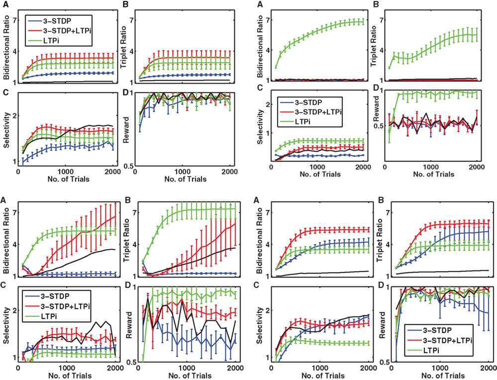
Figures A1–A4. Temporal evolution of network structure and performance. (A) Ratio of number of bidirectional connections to expected number. (B) Ratio of number of fully connected triplets to expected number. (C) Paired-stimulus selectivity averaged across network. (D) Mean reward obtained. All results depict the mean and standard error from four different network instantiations. Plasticity mechanisms are triplet-STDP (blue), combined triplet-STDP with LTPi (red) and LTPi alone (green). The black curve without error bars depicts one example of the worst performing network when parameters for structural plasticity were modified (setting R = 0.5) with triplet-STDP combined with LTPi. Figure A1: input probability = 1/5, 2 input groups. Figure A2: input probability = 1/20, 2 input groups. Figure A3: input probability = 1/20, 4 input groups. Figure A4: input probability = 1/20, 6 input groups.
The parameters used for structural plasticity were highly unconstrained, and chosen to ensure a very small fraction of synapses would be replaced per trial on average. To test how robust our results were to changes in these parameters, we simulated a single set of 25 input configurations with each parameter individually either halved or doubled in value. The results were remarkably robust to these changes as described in Table A1. The single parameter change that produced globally significant consequences, namely less clustering, after 400 trials was a reduction of the rate of structural plasticity by reducing R from 1 to 0.5. No results from simulations of this network for 2000 trials were globally significantly different from those with control parameters after 400 trials. Some example networks (which include the two most strongly altered by this parameter adjustment) are shown as the single black curve in Figures A1–A4. Analysis of the two worst cases (Figures A1 and A4) revealed that in these networks with R = 0.5, the number of synapses removed and replaced was more than 10-fold smaller than control. Thus our conclusion is that modification of parameters for structural plasticity can strongly alter the rate of structural plasticity (average number of synapses lost and replaced per trial) but does not alter the tendency of structural plasticity to enhance clustering.
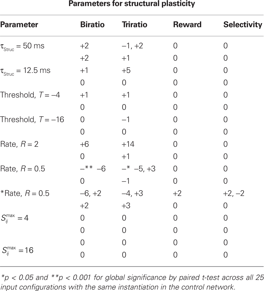
Table A1. Robustness of results to two-fold changes in structural plasticity parameters. For each parameter change from the control network, the upper row indicates number of network input configurations (out of 25) where the single instance of altered parameter differed from the 4 control instances at 5% significance (lower row at 0.2% significance) by 2-sample t-test, with ⩲ indicating improvement and – a worsening from control.
For each parameter change from the control network, the upper row indicates number of network input configurations (out of 25) where the single instance of altered-parameter differed from the four control instances at 5% significance (lower row at 0.2% significance) by two-sample t-test, with +indicating improvement and – a worsening from control. * Indicates p < 05 and **p < 001 for global significance by paired t-test across all 25 input configurations with the same instantiation in the control network.
Our standard network has different refractory properties for excitatory versus inhibitory cells; however, none of the results depended significantly (p > 0.05, paired t-test across four instantiations of each of 25 input configurations) on whether for inhibitory cells we set both of τref and τth to 1 ms or 2 ms (the latter matching excitatory cells).
Cells in our standard network included the NMDA conductance with a voltage-dependence that is observed in vitro (Jahr and Stevens, 1990). Removing the voltage-dependence had no significant effect on any of our results (p > 0.05, paired t-test across four instantiations of each of 25 input configurations).
The presence of structural plasticity in our networks can convert a bimodal distribution of synaptic strengths into a unimodal distribution (Figure 8). Such a result is in spite of the fact that the rule for triplet-STDP is additive, so should produce a bimodal distribution of synaptic strengths, whereas a multiplicative rule is known to produce a unimodal distribution (van Rossum et al., 2000). The distribution of synaptic strengths in our network is dominated by the cell-to-cell variation in mean synaptic strength, which produces a plaid-like striated structure to the matrix of connection strengths (Figure A5) as suggested by others (Koulakov et al., 2009).
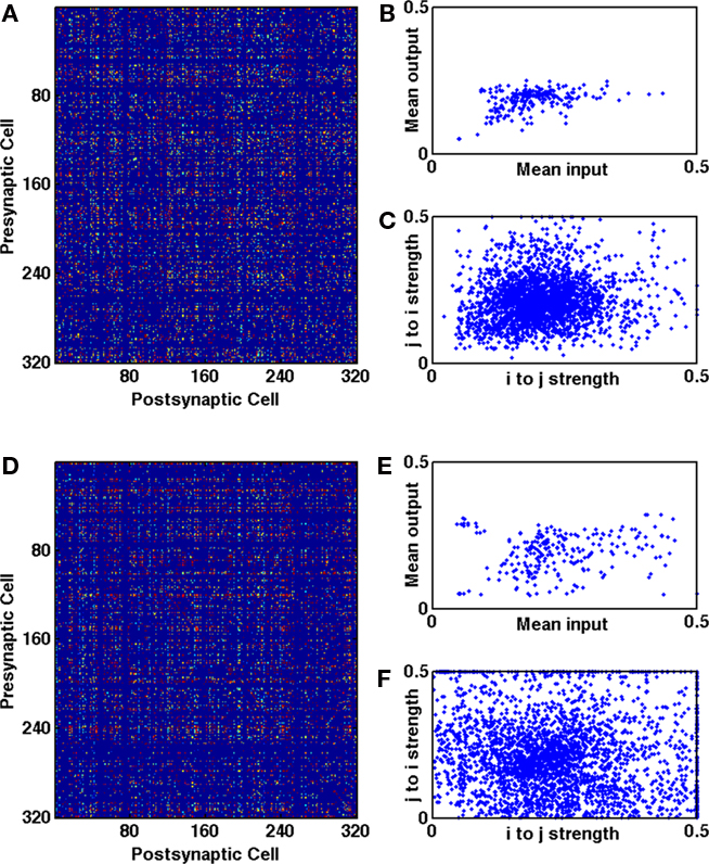
Figure A5. Synaptic strengths are not distributed randomly. (A,D) Matrix of connection strengths for an example network reveals plaid-like striations. (B,E) Mean of efferent synapses as a function of mean of afferent synapses for all cells in the network. (C,F) Strengths of reciprocal connections for all bidirectionally connected pairs of cells. (A–C) Additive plasticity produces positive correlations for global inputs and outputs across cells and across reciprocal connections [(B) Σ = 0.88, p < 10−100, (C) Σ = .11, p = 6 × 10⁻⁹]. (D–F) Multiplicative STDP produces a negative correlation between reciprocal connection strengths [(E) Σ = 0.57, p < 10−100, (F) Σ = −0.10, p = 2 × 10⁻⁸].
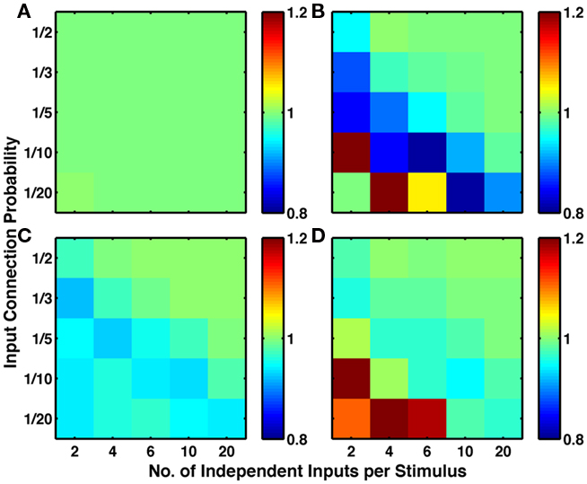
Figure A6. Bidirectional connections are stronger than unidirectional connections in networks with high degrees of clustering. Color indicates ratio of average strength of excitatory connections when the reciprocal connection is present to the strength of those with no reciprocal connection. All simulations include structural plasticity and homeostasis. (A) Simulations with no other functional plasticity show no effect (ratio remains at 1), while (C) simulations with LTPi alone show slightly weaker bidirectional connections caused by homeostasis on the excitatory synapses. By contrast, (B) simulations with triplet-STDP and (D) simulations with LTPi + triplet-STDP show that synapses partaking in a reciprocal connection are stronger than those forming a unidirectional connection in networks with a high degree of clustering (cf. Figures 5 and 6 of the main paper).
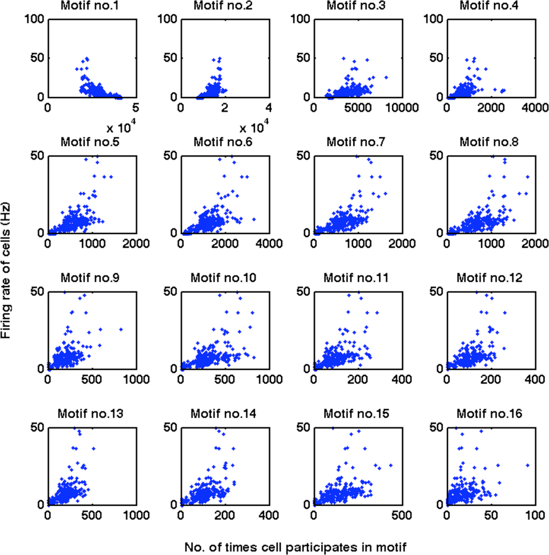
Figure A7. Cells with higher firing rates participate in more highly connected triplets. The local clustering coefficient of a cell is strongly correlated with its firing rate, as exhibited by the high correlation in the number of partially connected triplets (motifs 4–8) and fully connected triplets (motifs 10–16) with firing rate. Conversely, cells with low firing rate were more likely to be found in a fully disconnected triplet of cells (motif 1).
In networks with multiple functional plasticity mechanisms, the steady state synaptic strength is a dynamic equilibrium, whereby neither functional mechanism is at equilibrium alone, but the combined effects of different mechanisms cancel each other. When a Hebbian form of synaptic plasticity is combined with homeostasis by multiplicative synaptic scaling, the mean rate of initially highly active cells equilibrates at a level above the homeostatic goal rate, where the Hebbian increase in synaptic strengths is countered by a homeostatic decrease in synaptic strengths. When structural plasticity is present, these more active cells receive more inputs. Thus, the rate of the cell for equilibrium across plasticity mechanisms is reached at a lower synaptic strength per input – the total input to the cell that produces balance is reached with a lower individual synaptic strength, because more synapses are present. Thus the piling up of synaptic strengths at the upper bound, a cause of bimodality in the distribution, can be avoided.
Keywords: structural plasticity, connectivity, Hebbian learning, network, simulation, correlations, STDP, inhibitory plasticity
Citation: Bourjaily MA and Miller P (2011) Excitatory, inhibitory, and structural plasticity produce correlated connectivity in random networks trained to solve paired-stimulus tasks. Front. Comput. Neurosci. 5:37. doi: 10.3389/fncom.2011.00037
Received: 15 October 2010; Accepted: 02 August 2011;
Published online: 12 September 2011.
Edited by:
Stefano Cardanobile, University of Freiburg, GermanyReviewed by:
Matthieu Gilson, Bernstein Center Freiburg, GermanyCopyright: © 2011 Bourjaily and Miller. This is an open-access article subject to a non-exclusive license between the authors and Frontiers Media SA, which permits use, distribution and reproduction in other forums, provided the original authors and source are credited and other Frontiers conditions are complied with.
*Correspondence: Paul Miller, Volen National Center for Complex Systems, MS013 Brandeis University, 415 South Street, Waltham, MA 02454, USA. e-mail:cG1pbGxlckBicmFuZGVpcy5lZHU=
Disclaimer: All claims expressed in this article are solely those of the authors and do not necessarily represent those of their affiliated organizations, or those of the publisher, the editors and the reviewers. Any product that may be evaluated in this article or claim that may be made by its manufacturer is not guaranteed or endorsed by the publisher.
Research integrity at Frontiers

Learn more about the work of our research integrity team to safeguard the quality of each article we publish.