Experimental estimation of sample entropy in a semiconductor laser with optical feedback for random number generation

Estimating the entropy rate of physical random number generators with uncertainty is crucial for information security applications. We evaluate the sample entropy of chaotic temporal waveforms generated experimentally by a semiconductor laser with time-delayed optical feedback. We demonstrate random number generation with uncertainty using a quantitative measurement of the entropy rate.

1 Introduction

Physical random number generators have attracted increasing interest for engineering applications in information security and numerical simulations. Physical random number generators are based on physical random phenomena, and the sequences generated from physical random number generators are, in principle, unpredictable and irreproducible (Uchida, 2012). However, the speed of physical random number generators based on noise in electronic circuits is limited to tens of megabits per second (Mb/s). To enhance the generation speed, physical random number generators based on chaotic semiconductor lasers have been proposed (Uchida et al., 2008), where physical random numbers are generated at a rate of gigabits per second (Gb/s). Several post-processing methods have been applied to improve the randomness of the generated bit sequences, such as least significant bit (LSB) extraction and bit-order reversal (Akizawa et al., 2012). Using these post-processing methods, the speed of random number generation based on chaotic semiconductor lasers can be improved at a rate of up to terabits per second (Tb/s) (Sakuraba et al., 2015). Real-time random number generation uses a photonic integrated circuit and FPGA (Ugajin et al., 2017). Recently, physical random number generation at a rate of 250 Tb/s was reported using the spatiotemporal dynamics of a specially designed semiconductor laser with curved facets (Kim et al., 2021).

An important issue in high-speed random number generation is that its speed of random number generation may exceed the entropy rate (i.e., the uncertainty generation rate) of the physical entropy sources (Hart et al., 2017). High-speed random number generation can be achieved by introducing complex post-processing; however, the entropy rate cannot be enhanced by post-processing. The entropy rate of physical random number generators must be evaluated to ensure the uncertainty and unpredictability of the generated bit sequences (Hart et al., 2017).

Several measures of entropy rate have been reported in the literature. One of the most common entropy measures is the Kolmogorov-Sinai (KS) entropy in nonlinear dynamical systems (Eckmann and Ruelle, 1985). The KS entropy can be calculated from the sum of positive Lyapunov exponents. However, a numerical model is required to obtain a reliable estimation of multiple Lyapunov exponents (i.e., the Lyapunov spectrum), and linearized equations of the numerical model are used to calculate the KS entropy (Uchida, 2012). Therefore, it is difficult to estimate the KS entropy obtained from experimentally measured chaotic temporal waveforms using physical entropy sources.

The (ε,τ) entropy has been reported as a measure of entropy rate, which can be directly calculated from experimentally obtained temporal waveforms (Cohen and Procaccia, 1985; Gaspard and Wang, 1993; Kawaguchi et al., 2021). The (ε,τ) entropy requires the discretization and quantization of temporal waveforms using the quantization interval ε of the amplitude and the sampling interval τ of the time. This is useful for estimating the entropy of the experimental data because they are already discretized and quantized.

One of the issues of the (ε,τ) entropy is the fact that a large number of sampling data is required when ε and τ are small. In addition, the number of data points within the distance ε is diminished when the length of reference vectors d is increased for a finite number of sampled data. Therefore, revised versions of the (ε,τ) entropy have been proposed to reduce the computational cost, such as the sample entropy and the approximate entropy (Richman and Moorman, 2000; Yentes et al., 2013), where the algorithms of the entropy estimation process are simplified. Statistical tests of entropy estimation for physical random number generators were proposed by the National Institute of Standards and Technology (NIST) Special Publication (SP) 800–90B (Barker and Kelsey, 2016).

The estimation of entropy rate in chaotic laser dynamics has been investigated (Hagerstrom et al., 2015; Li et al., 2016). The estimation of the (ε,τ) entropy has been reported using chaotic temporal waveforms generated from a semiconductor laser with optical injection (Kawaguchi et al., 2021). In addition, the entropy rate of white chaos generated from optical heterodyne signals was evaluated using NIST SP 800-90B (Yoshiya et al., 2020). However, an entropy evaluation method for photonic dynamic systems is yet to be developed. In particular, simplified techniques, such as sample entropy, have not been applied to the chaotic dynamics in semiconductor lasers with time-delayed optical feedback. Therefore, it is crucial to develop a concrete method for obtaining a simple and reliable estimation of the entropy rate from experimental data.

In this study, we experimentally evaluate the entropy rate of chaotic temporal waveforms generated by a semiconductor laser with time-delayed optical feedback. We focus on the sample entropy and compare it with other entropy for reliable estimation. We generate random bit sequences from a chaotic semiconductor laser and evaluate the randomness of the bit sequences and the entropy rate of the physical source to guarantee the random number generation with uncertainty.

2 Entropy rate estimation

2.1 Methods for estimation of (ε,τ) entropy and sample entropy

In this section, we describe the calculation method of the (ε,τ) entropy and sample entropy. We prepare a chaotic temporal waveform of laser intensity generated by a semiconductor laser with optical feedback (Uchida, 2012). The temporal waveform is sampled at a sampling interval τ, as shown in Figure 1. The discrete time t is represented as iτ (i = 1,2, …, N, where Nτ is the total length of the temporal waveform). The amplitude of the temporal waveform is quantized at a quantization interval ε. Next, we randomly select a sampling point $x\left(i\tau \right)$ in the temporal waveform, which is called the reference data, and prepare a reference vector ${\mathit{x}}_{\mathit{i}}^{\mathit{d}}$ with vector length d. The reference vector ${\mathit{x}}_{\mathit{i}}^{\mathit{d}}$ is expressed as follows:

${\mathit{x}}_{\mathit{i}}^{\mathit{d}}=\left[x\left(i\tau \right),x\left(\left(i+1\right)\tau \right),\dots ,x\left(\left(i+d-1\right)\tau \right)\right](1)$

Figure 1

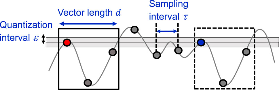
Figure 1. Schematic of the calculation of the (ε,τ) entropy and the sample entropy.

The distance between two vectors ${\mathit{x}}_{\mathit{i}}^{\mathit{d}}$ and ${\mathit{x}}_{\mathit{j}}^{\mathit{d}}$ ($i\ne j$) is defined by calculating the maximum value of the difference in each vector component as follows.

$dist[{\mathit{x}}_{\mathit{i}}^{\mathit{d}},{\mathit{x}}_{\mathit{j}}^{\mathit{d}}]=\mathit{max}\left[\begin{array}{c}\left|x\left(i\tau \right)-x\left(j\tau \right)\right|,\left|x\left(\left(i+1\right)\tau \right)-x\left(\left(j+1\right)\tau \right)\right|,\dots ,\\ \left|x\left(\left(i+d-1\right)\tau \right)-x\left(\left(j+d-1\right)\tau \right)\right|\end{array}\right](2)$

We calculate the probability $A_i^d$ of the existence of the neighboring vectors within the distance ε as follows.

$A_i^d=\frac{Number\left[{\mathit{x}}_{\mathit{i}}^{\mathit{d}};dist[{\mathit{x}}_{\mathit{i}}^{\mathit{d}},{\mathit{x}}_{\mathit{j}}^{\mathit{d}}]\le \epsilon \right]}{Number\left[{\mathit{x}}_{\mathit{i}}^{\mathit{d}}\right]},(3)$

where $Number\left[[{\mathit{x}}_{\mathit{i}}^{\mathit{d}};dist[{\mathit{x}}_{\mathit{i}}^{\mathit{d}},{\mathit{x}}_{\mathit{j}}^{\mathit{d}}]\le \epsilon \right]]$ represents the number of the neighboring vectors within the distance ε and $Number\left[[{\mathit{x}}_{\mathit{i}}^{\mathit{d}}\right]]$ indicates the total number of the vectors ${\mathit{x}}_{\mathit{i}}^{\mathit{d}}$. The value of $A_i^d$ is calculated for different sampling points i. The average of the base 2 (binary) logarithm of $A_i^d$ is calculated for the (ε,τ) entropy as follows.

$A^d=-\frac{1}{R}{\displaystyle \sum _{i=1}^R}{\log }_2{A}_i^d\left(\text{for\hspace{0.17em}}\left(\epsilon ,\tau \right)\text{\hspace{0.17em}entropy}\right),(4)$

where $R$ denotes the number of reference data points. By contrast, for the sample entropy, the average of $A_i^d$ is calculated first, and the logarithm of the average value is calculated as follows:

$A^d=-{\log }_2\left(\frac{1}{R}{\displaystyle \sum _{i=1}^R}{A}_i^d\right)\left(\text{for\hspace{0.17em}sample\hspace{0.17em}entropy}\right)(5)$

The entropy $E$ is obtained from the difference between $A^d$ and $A^{d+1}$ as follows.

$E=A^d-A^{d+1}\left[\text{bit}/\text{sample}\right](6)$

The entropy rate is obtained by dividing the entropy $E$ by τ as follows.

$h=\frac{E}{\tau }\left[\text{bit}/\text{second}\right](7)$

The entropy rate relies on both the quantization and sampling intervals (ε and τ) of chaotic temporal waveforms and the vector length d. It has been known that the (ε,τ) entropy converges to the KS entropy under the limit of $\epsilon \to 0$ and $\tau \to 0$ (Cohen and Procaccia, 1985; Gaspard and Wang, 1993).

For the (ε,τ) entropy, when $\epsilon$ is set to be too small, $A_i^d$ can be zero, and Eq. 4 diverges to negative infinity. To avoid this issue, the reference vector is considered as the neighboring vector, so that $Number\left[[{\mathit{x}}_{\mathit{i}}^{\mathit{d}};dist[{\mathit{x}}_{\mathit{i}}^{\mathit{d}},{\mathit{x}}_{\mathit{j}}^{\mathit{d}}]\le \epsilon \right]]$ is one or larger. By contrast, this modification is not required for sample entropy because the average of $A_i^d$ is first calculated, and the logarithm of the averaged probability is obtained. Therefore, the sample entropy is expected to be more reliable for a large d.

3 Experimental results

3.1 Experimental setup and chaotic temporal waveforms

Figure 2 shows the experimental setup for generating chaotic temporal waveforms in a semiconductor laser with time-delayed optical feedback. A distributed-feedback (DFB) semiconductor laser (NTT Electronics, KELD1C5GAAA) was used as a light source. The injection current of the semiconductor laser was set to 38.5 mA (3.5 times the lasing threshold). A fiber reflector was used to produce time-delayed optical feedback for the laser to generate chaotic laser outputs. The feedback delay time was set to 25.0 ns. The feedback power is set to 58 μW, which corresponds to the feedback ratio of 0.008 compared with the laser power. The chaotic temporal dynamics of the laser intensity can be obtained using time-delayed optical feedback. The chaotic temporal waveforms were converted into electric signals using a photoreceiver (Newport, 1554-B, 12 GHz bandwidth). The converted electric signals were measured using a digital oscilloscope (Tektronix, DPO73304D, 33 GHz bandwidth, maximum sampling rate of 100 GigaSample/s (GS/s), and 8-bit vertical resolution). The sampled data were stored on a digital oscilloscope and were used to estimate the entropy rate. The radio frequency (RF) spectra of the electric signals were observed using an RF spectrum analyzer (Agilent Technologies, N9010A-544, 44 GHz bandwidth).

Figure 2

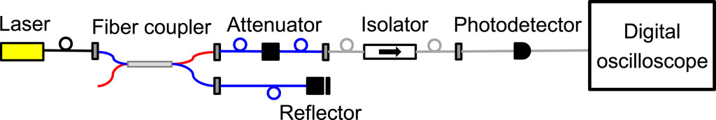
Figure 2. Experimental setup for generating chaotic temporal waveforms in a semiconductor laser with time-delayed optical feedback.

Figure 3 shows the experimental results for the chaotic temporal waveform of the laser intensity, the corresponding RF spectrum, and a histogram of the amplitude of the chaotic temporal waveform. Chaotic temporal waveforms are obtained and broad spectral components are observed in the RF spectrum. In addition, the histogram of the chaotic temporal waveforms appears to be asymmetric, as shown in Figure 3C. This asymmetry can be eliminated by subtracting the original chaotic signal from its time-delayed signal (Reidler et al., 2009) to improve the statistical characteristics of the generated random bits. However, our goal is to estimate the entropy rate of the original chaotic signal, and we use the chaotic data with the asymmetric histogram shown in Figure 3C. The chaotic temporal waveforms are acquired so that their standard deviation is set to σ = 32 in the 8-bit vertical resolution with a range of [-128, 127], where the histogram is ranged within ±4σ.

Figure 3

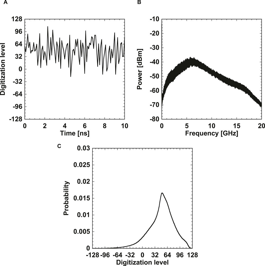
Figure 3. Experimental results of (A) the chaotic temporal waveform of the laser intensity, (B) the corresponding radio-frequency (RF) spectrum, and (C) the histogram of the amplitude of the chaotic temporal waveform.

3.2 Entropy rate estimation

We estimate the (ε,τ) entropy and sample entropy of the experimentally obtained chaotic temporal waveforms in Figure 3. The parameter values for the entropy estimation are set as follows: The sampling interval of τ = 100 ps (10 GHz in frequency), the quantization resolution of ε = 2^8-n for Most Significant Bits n (MSBs n) in the 8-bit vertical resolution with the range of [-128, 127], the number of sampling data of N = 10⁹, and the number of reference data of R = 10⁵. We use a notation of “MSBs n” for multiple bits generated from the 1st, 2nd, …, and nth MSB at one sampling point. The remaining bits from the (n+1)-th MSB, …, and 8th MSB are discarded from the original 8-bit data. The 8th MSB corresponds to the 1st least significant bit (LSB) of 8-bit data. For example, MSBs 3 corresponds to three bits, including the 1st, 2nd, and 3rd MSB of the 8-bit data. We also use a notation of “the nth MSB” for a single bit generated from only the nth MSB at one sampling point (see Section 4.2).

Figure 4 shows the comparison of the (ε,τ) entropy and the sample entropy for different MSBs n (i.e., different ε = 2^8-n) when the vector length d is increased. τ is fixed at 100 ps. In Figure 4A, the (ε,τ) entropy decreases for a large d and large MSBs n (a small ε). Plateaus are not observed when d or n increases. By contrast, in Figure 4B, the sample entropy shows large plateau regions for all MSBs. The entropy at the plateau can be considered as the estimated value of the sample entropy. Therefore, the sample entropy can be estimated even for large MSBs n, and it is more reliable than the (ε,τ) entropy.

Figure 4

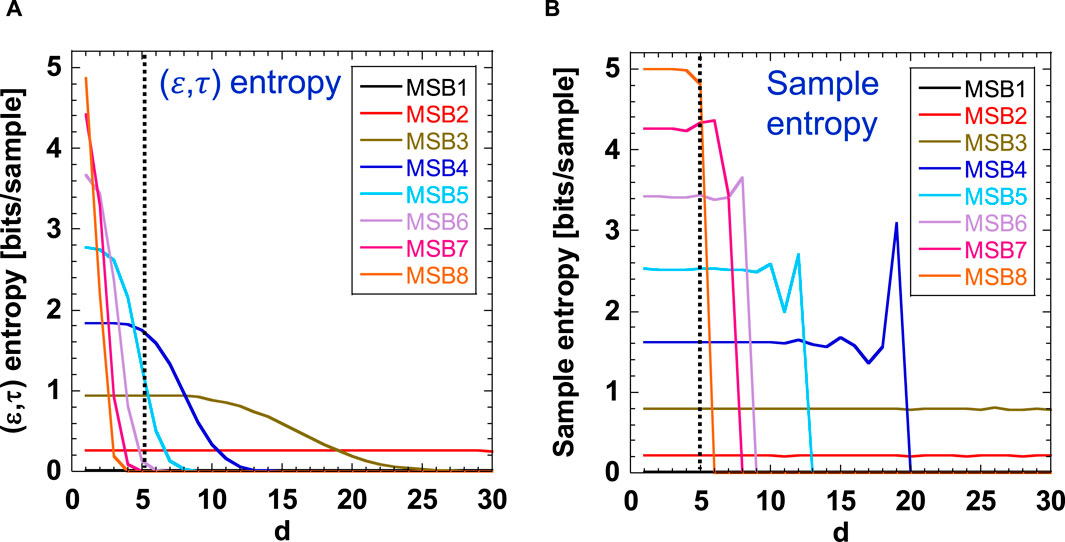
Figure 4. Comparison of (A) the (ε,τ) entropy and (B) the sample entropy for different MSBs n (different ε = 2^8-n) when the vector length d is increased. The black dotted line corresponds to d =5, whose crossing points are used to estimate the value of entropy for different MSBs n.

To investigate the difference between Figures 4A, B, we plot the probability of having the value of $A_i^d=0$ in $R$ reference data when d is increased for MSBs 4, as shown in Figure 5. In Figure 5A, the (ε,τ) entropy for MSBs 4 decreases as the probability of $A_i^d=0$ increases for a large d, and the (ε,τ) entropy becomes zero when the probability of $A_i^d=0$ reaches one. Therefore, it is difficult to correctly estimate the (ε,τ) entropy when the two neighboring vectors within the distance ε do not exist. By contrast, in Figure 5B, the sample entropy remains constant with an increase in d, even though the probability of $A_i^d=0$ increases and is close to one. This result originates from the average calculation of $A_i^d$ for $R$ reference data before creating a logarithm, as shown in Eq. 5. Therefore, the sample entropy is more robust when the number of neighboring vectors within the distance ε is reduced for a large number of d and MSBs n.

Figure 5

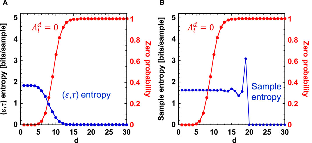
Figure 5. (A) (ε,τ) entropy and (B) the sample entropy for MSBs 4 when the vector length d is increased (the blue curve). The probability of having the value of $A_i^d=0$ in $R$ reference data are also plotted (the red curve).

From Figures 4, 5, we found that the sample entropy is less dependent on MSBs n than the (ε,τ) entropy. This result is explained by the comparison of Figures 5A, B, where the (ε,τ) entropy decreases as the probability of $A_i^d=0$ increases, while the sample entropy remains the same value. Therefore, sample entropy can provide an entropy measurement for larger MSBs n. We consider this characteristic to be a general feature of other data used for entropy measurements.

Next, we change the quantization interval ε and the corresponding MSBs n. Figure 6 shows the comparison of the (ε,τ) entropy and the sample entropy obtained from the values of the plateaus shown in Figures 4A, B, where the vector length is set to d = 5. In Figure 6, the (ε,τ) entropy can be estimated reliably up to MSBs 3, because of the lack of the plateaus in Figure 4A. By contrast, the sample entropy can be obtained up to MSBs 8 (i.e., all 8 bits), as shown in Figure 4B. Figure 6 shows the maximum sample entropy (5.0) for MSBs 8. In addition, a sample entropy of more than one bit can be obtained for MSBs 4 or more MSBs. This result indicates that random number generation with uncertainty (i.e., entropy generation) can be achieved using one bit generated from MSBs 4 or larger.

Figure 6

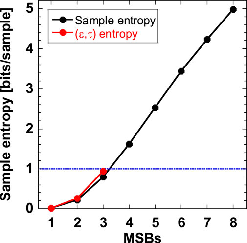
Figure 6. Comparison of the (ε,τ) entropy (the red curve) and the sample entropy (the black curve) obtained from the values of the plateaus shown in Figures 4A, B, where the vector length is set to d = 5. The blue dotted line indicates the sample entropy of 1.

We also change the sampling interval τ, corresponding to the inverse of the sampling frequency f_s (=1/τ). Figure 7 shows the sample entropy for different f_s values when n is changed. The quantization interval ε = 2^8-n is also changed. The vector length is set to d = 5. The sample entropy increases for large MSBs n. In addition, higher entropy is obtained when f_s is reduced. The sample entropy is saturated when f_s is reduced to 10 GS/s or smaller (τ = 100 ps or larger).

Figure 7

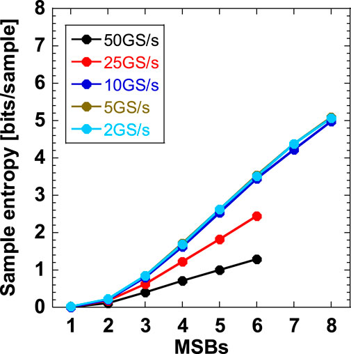
Figure 7. Sample entropy for different sampling frequency f_s (=1/τ) when MSBs n is changed. The quantization interval ε = 2^8-n is also changed. The vector length is set to d = 5.

From Figure 7, the entropy rate is calculated by multiplying the estimated sample entropy by the sampling frequency. We can obtain an entropy up to MSBs 6 for f_s = 25 and 50 GS/s, and MSBs 8 for 10 GS/s or less, because of the existence of plateaus, as shown in Figure 4B. In Figure 7, a sample entropy of 5.0 at f_s = 10 GS/s is obtained for MSBs 8, and the corresponding entropy rate is 50 GHz (=5.0 $\times$ 10 GS/s). In another case, a sample entropy of 1.0 at 50 GS/s is obtained for MSBs 5, and the entropy rate is 50 GHz (=1.0 $\times$ 50 GS/s) as well. The same entropy rate can be obtained for different combinations of the sampling rate and number of MSBs. Therefore, an entropy rate of 50 GHz is obtained for the chaotic temporal waveforms of the laser intensity generated in the experiment.

3.3 Validation of sample entropy

To confirm the validity of the sample entropy estimation, we use the de facto standard of statistical tests of entropy evaluation for physical random number generators, known as NIST SP 800-90B (Barker and Kelsey, 2016). We obtain signals with n-bit vertical resolutions (MSBs n) for the NIST SP 800-90B tests and evaluate the minimum entropy of the n-bit signals generated from the physical entropy sources. The statistical tests consist of ten different entropy evaluations. The minimum value of the entropy evaluations in the ten tests is selected as the final estimate. We select the MSBs n of the 8-bit data (n bits) and evaluate the entropy of MSBs n. The maximum entropy corresponds to n for the data of MSBs n. We use 1 Mega point data to evaluate the entropy using NIST SP 800-90B.

Figure 8 compares the sample entropy and minimum entropy values obtained from NIST SP 800-90B. The sampling frequency is set to f_s = 10 GS/s (τ = 100 ps). Both of the entropy values increase as the number of MSBs increases. In addition, the sample entropy is smaller than that obtained using NIST SP 800-90B for all the MSBs. This result indicates that the sample entropy is underestimated compared with the entropy of NIST SP 800-90B. The sample entropy is close to the entropy of NIST SP 800-90B for MSBs 5 and 6. The overall characteristics coincides between the sample entropy and entropy of NIST SP 800-90B.

Figure 8

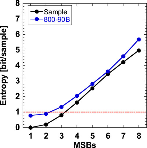
Figure 8. Comparison of the sample entropy (the black curve) and the minimum value of the entropy obtained from NIST SP 800-90B (the blue curve). The sampling frequency is set to f_s = 10 GS/s (τ = 100 ps).

4 Random number generation with uncertainty

4.1 Estimation of entropy of noise signals

In this section, we evaluate the entropy rate of chaotic temporal waveforms used for physical random number generation. First, we evaluate the entropy of the noise signals to distinguish the origin of the entropy from stochastic noise and deterministic chaos. Figure 9A shows the temporal waveform of the experimentally obtained noise signals. The noise signal is detected using the digital oscilloscope and the photoreceiver without optical injection from the semiconductor laser (see Figure 2). The vertical range of the amplitude is set to be the same as that for the chaotic signals, as shown in Figure 3A.

Figure 9

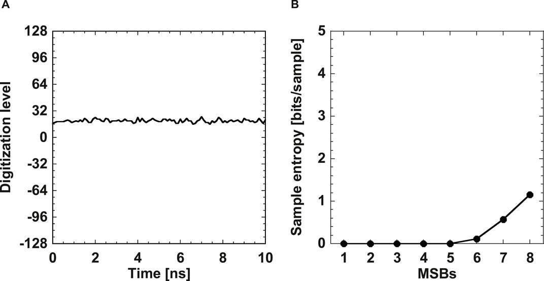
Figure 9. (A) Temporal waveform and (B) sample entropy of the noise signal obtained in experiment. The vector length is set to d = 5.

Figure 9B shows the sample entropy of the noise signals obtained in the experiment. The sample entropy is zero between MSBs 1 and 5, and the entropy for more than MSBs 5 has a positive value. Here, MSBs 5 consists of the 1st, 2nd, …, and 5th MSB, and the 6th, 7th, and 8th MSB, which are the most sensitive to noise, are not included in MSBs 5. This result indicates that entropy originating from stochastic noise exists in the data of MSBs 6 or larger. Therefore, we use data of MSBs 5 or less for physical random number generation to avoid the contribution of stochastic noise to entropy.

4.2 Statistical evaluation of random number generation

We generate physical random bit sequences using minimum post-processing based on a bitwise XOR operation between the original and time-delayed signals (Takahashi et al., 2014; Sakuraba et al., 2015). First, chaotic temporal waveforms are sampled and converted into 8-bit signals. The 8-bit signal and its time-delayed signal are stored, and a bitwise XOR operation is performed between the original and time-delayed signals. The delay time is set to 3.0 ns (30 sampling points at the sampling interval of τ = 100 ps) to avoid the correlation between the original and time-delayed chaotic signals. The nth MSB of the resultant bits is extracted and combined with the signals sampled at different times as random bit sequences. Note that the nth MSB indicates only one bit at the nth bit counted from the 1st MSB, which differs from MSBs n used in the previous sections (i.e., MSBs n include the 1st, 2nd, …, and nth MSB). One bit obtained at the nth MSB is combined with different sampled data points, and N bits are generated from N sampled data points for each nth MSB.

To evaluate the statistical randomness of the generated bit sequences, we use NIST SP 800-22 tests (Rukhin et al., 2010), which are de facto standard tests for the statistical evaluation of random numbers. These statistical tests evaluate the statistical randomness of the bits (0 or 1) generated from the random number generators. NIST SP 800-22 consists of 15 statistical tests, and the random bits that pass all statistical tests are considered high-quality random numbers.

Figure 10A shows the results of NIST SP 800-22 at a sampling frequency of f_s = 50 GS/s. The bit sequences generated from the 5th MSB or higher can pass all 15 tests However, the bit sequences generated from the 4th MSB or less fails to some tests. This result indicates that the 5th MSB can be used as a random number. Figure 10B shows the results of NIST SP 800-22 for different sampling frequencies ranging from f_s = 2 to 25 GS/s. The 4th MSB or higher can pass all NIST tests in these cases. Therefore, the 4th MSB is also useful as a random number when f_s is reduced to 25 GS/s or less.

Figure 10

Figure 10. Result of NIST SP 800-22 for the bit sequences generated from the nth MSB at the sampling frequency of (A) f_s = 50 GS/s and (B) f_s = 2, 5, 10, and 25 GS/s. All 15 tests need to be passed for high-quality random numbers.

5 Discussion

From the results in Figures 7, 9, 10, we consider that data with the 4th or 5th MSB are useful for random number generation with uncertainty. From Figure 7, an entropy greater than one can be generated for MSBs 5 sampled at 50 GS/s, and for MSBs 4 sampled at 25 GS/s or less. Therefore, at least one random bit can be extracted from the data. From Figure 9, we must avoid data of MSBs 6 or larger to distinguish the origin of the entropy from stochastic noise and deterministic chaos. From Figure 10, we can confirm that all NIST SP 800-22 tests are passed for the 5th MSB sampled at 50 GS/s and the 4th MSB sampled at 25 GS/s or less. Data of small MSBs correlate with neighboring bits and that the randomness of these bits is not sufficiently high. By contrast, data of large MSBs are affected by stochastic noise, which can be avoided when we consider the contribution of entropy only from a deterministic chaotic signal and not from stochastic noise. Therefore, an intermediate MSB (e.g., the 4th or 5th MSB) is useful for extracting one random bit with uncertainty.

Our results show that an entropy of more than one bit can be obtained from the bit sequences generated from MSBs 5, which includes the 1st, 2nd, …, and 5th MSB, as measured by NIST SP 800-90B tests. In addition, the bit sequences generated from the 4th or 5th MSB can pass the statistical tests of randomness, as measured by the NIST SP 800-22 tests. The entropy measurement using NIST SP 800-90B requires n-bit data (n ≥ 1), whereas the measurement of statistical bias using NIST SP 800-22 requires 1-bit data. Therefore, different data formats are used for the measurement of entropy and statistical bias.

The entropy can be generated by a small change in two vectors ${\mathit{x}}_{\mathit{i}}^{\mathit{d}}$ and ${\mathit{x}}_{\mathit{j}}^{\mathit{d}}$ $\left(i\ne j\right)$ for MSBs n data when the vector length increases from d to d+1, defined by Eq. 6. In most cases, the distance of one of the elements between the two vectors is slightly over the quantization interval ε = 2^8-n when entropy is generated, described as in Eq. 3. This indicates that uncertainty of the two vectors appears at the least significant bit of the MSB n data (i.e., the nth MSB). Therefore, we consider that the nth MSB must contain most uncertainty among other bits of MSBs n when MSBs n data can pass NIST SP 800-90B. We thus recommend using the 4th MSB (sampled at 25 GS/s or less) or 5th MSB (sampled at 50 GS/s) to generate random bit sequences with both uncertainty and no statistical bias.

We compare our results to those of a previous study (Kawaguchi et al., 2021). In the previous work, the entropy was calculated only from MSBs 1 to 3, because they used the (ε,τ) entropy. As seen in Figure 4 of this study, the estimation of entropy for larger MSBs n is difficult by using the (ε,τ) entropy. Instead, we perform the estimation of entropy for all MSBs n (1 ≤ n ≤ 8) by using the sample entropy. We have not obtained the same result as in the previous work quantitatively (i.e., the use of the 3rd MSB is the best for random number generation in the previous work, whereas the use of the 4th or 5th MSB is the best in this study). However, the conclusions of the previous and current studies are qualitatively consistent, that is, an intermediate MSB of 8-bit data is useful for physical random number generation with uncertainty.

In this study, we consider only the additive noise originating from the measurement equipment (e.g., noise in the photodetector, electric amplifier, and digital oscilloscope). We do not focus on the intrinsic multiplicative noise in laser dynamics (e.g., spontaneous emission noise). The inclusion of intrinsic noise is an important topic that will be investigated in future work.

6 Conclusion

We experimentally evaluated the sample entropy of chaotic temporal waveforms in a semiconductor laser with optical feedback. We found the reliable estimation of the sample entropy even for a large vector length d, whereas the estimation of the (ε,τ) entropy is limited for a large d. We estimated the sample entropy at different sampling intervals and determined the conditions for random number generation with an entropy of more than one bit at an entropy rate of 50 GHz. The validity of the sample entropy was confirmed by a comparison with the results of NIST SP 800-90B. We also generated random bit sequences and evaluated their statistical randomness of the generated bits. All NIST SP 800-22 tests were passed for the bit sequences generated from the 5th MSB sampled at 50 GS/s and the 4th MSB sampled at 25 GS/s. Random number generation with more than one-bit of entropy was demonstrated using the 4th or 5th MSB as a physical random number generator with uncertainty.

The methodology for estimating the sample entropy is promising for evaluating physical random number generators based on various physical entropy sources. Physical random number generators with uncertainty are required for information-security and cryptography applications.

Data availability statement

The raw data supporting the conclusion of this article will be made available by the authors, without undue reservation.

Author contributions

TO: Data curation, Formal Analysis, Investigation, Resources, Software, Visualization, Writing–review and editing. KK: Data curation, Formal Analysis, Investigation, Software, Validation, Writing–review and editing. AU: Conceptualization, Funding acquisition, Investigation, Methodology, Project administration, Supervision, Writing–original draft, Writing–review and editing.

Funding

The author(s) declare that financial support was received for the research, authorship, and/or publication of this article. This work was supported in part by Grants-in-Aid for Scientific Research from the Japan Society for the Promotion of Science (JSPS KAKENHI; Grant Nos. JP19H00868, JP20K15185, and JP22H05195), JST CREST, Japan (JPMJCR17N2), and the Telecommunications Advancement Foundation.

Conflict of interest

The authors declare that the research was conducted in the absence of any commercial or financial relationships that could be construed as a potential conflict of interest.

The author(s) declared that they were an editorial board member of Frontiers, at the time of submission. This had no impact on the peer review process and the final decision.

Publisher’s note

All claims expressed in this article are solely those of the authors and do not necessarily represent those of their affiliated organizations, or those of the publisher, the editors and the reviewers. Any product that may be evaluated in this article, or claim that may be made by its manufacturer, is not guaranteed or endorsed by the publisher.

References

Akizawa, Y., Yamazaki, T., Uchida, A., Harayama, T., Sunada, S., Arai, K., et al. (2012). Fast random number generation with bandwidth-enhanced chaotic semiconductor lasers at 8 × 50 Gb/s. IEEE Photonics Technol. Lett. 24 (12), 1042–1044. doi:10.1109/lpt.2012.2193388

CrossRef Full Text | Google Scholar

Barker, E., and Kelsey, J. (2016). Recommendation for the entropy sources used for random bit generation. NIST Draft Special Publication., 800–90B. second draft.

Google Scholar

Cohen, A., and Procaccia, I. (1985). Computing the Kolmogorov entropy from time signals of dissipative and conservative dynamical systems. Phys. Rev. A 31 (3), 1872–1882. doi:10.1103/physreva.31.1872

PubMed Abstract | CrossRef Full Text | Google Scholar

Eckmann, J. P., and Ruelle, D. (1985). Ergodic theory of chaos and strange attractors. Rev. Mod. Phys. 57, 617–656. doi:10.1103/revmodphys.57.617

CrossRef Full Text | Google Scholar

Gaspard, P., and Wang, X.-J. (1993). Noise, chaos, and (ε, τ)-entropy per unit time. Phys. Rep. 235 (6), 291–343. doi:10.1016/0370-1573(93)90012-3

CrossRef Full Text | Google Scholar

Hagerstrom, A. M., Murphy, T. E., and Roy, R. (2015). Harvesting entropy and quantifying the transition from noise to chaos in a photon-counting feedback loop. Proc. Natl. Acad. Sci. USA. 112 (30), 9258–9263. doi:10.1073/pnas.1506600112

PubMed Abstract | CrossRef Full Text | Google Scholar

Hart, J. D., Terashima, Y., Uchida, A., Baumgartner, G. B., Murphy, T. E., and Roy, R. (2017). Recommendations and illustrations for the evaluation of photonic random number generators. Apl. Photonics 2 (9), 090901. doi:10.1063/1.5000056

CrossRef Full Text | Google Scholar

Kawaguchi, Y., Okuma, T., Kanno, K., and Uchida, A. (2021). Entropy rate of chaos in an optically injected semiconductor laser for physical random number generation. Opt. Express 29, 2442. doi:10.1364/oe.411694

PubMed Abstract | CrossRef Full Text | Google Scholar

Kim, K., Bittner, S., Zeng, Y., Guazzotti, S., Hess, O., Wang, Q. J., et al. (2021). Massively parallel ultrafast random bit generation with a chip-scale laser. Science 371, 948–952. doi:10.1126/science.abc2666

PubMed Abstract | CrossRef Full Text | Google Scholar

Li, X.-Z., Zhuang, J.-P., Li, S.-S., Gao, J.-B., and Chan, S.-C. (2016). Randomness evaluation for an optically injected chaotic semiconductor laser by attractor reconstruction. Phys. Rev. E 94, 042214. doi:10.1103/physreve.94.042214

PubMed Abstract | CrossRef Full Text | Google Scholar

Reidler, I., Aviad, Y., Rosenbluh, M., and Kanter, I. (2009). Ultrahigh-speed random number generation based on a chaotic semiconductor laser. Phys. Rev. Lett. 103, 024102. doi:10.1103/physrevlett.103.024102

PubMed Abstract | CrossRef Full Text | Google Scholar

Richman, J. S., and Moorman, J. R. (2000). Physiological time-series analysis using approximate entropy and sample entropy. Am. J. Physiology. Heart Circulatory Physiology 278, H2039–H2049. doi:10.1152/ajpheart.2000.278.6.h2039

PubMed Abstract | CrossRef Full Text | Google Scholar

Rukhin, A., Soto, J., Nechvatal, J., Smid, M., Barker, E., Leigh, S., et al. (2010). National Institute of standards and Technology (NIST), Special Publication 800-22, revision 1a.

Google Scholar

Sakuraba, R., Iwakawa, K., Kanno, K., and Uchida, A. (2015). Tb/s physical random bit generation with bandwidth-enhanced chaos in three-cascaded semiconductor lasers. Opt. Express 23 (2), 1470–1490. doi:10.1364/oe.23.001470

PubMed Abstract | CrossRef Full Text | Google Scholar

Takahashi, R., Akizawa, Y., Uchida, A., Harayama, T., Tsuzuki, K., Sunada, S., et al. (2014). Fast physical random bit generation with photonic integrated circuits with different external cavity lengths for chaos generation. Opt. Express 22 (10), 11727–11740. doi:10.1364/oe.22.011727

PubMed Abstract | CrossRef Full Text | Google Scholar

Uchida, A. (2012). Optical Communication with Chaotic Lasers, Applications of Nonlinear Dynamics and Synchronization. Weinheim: Wiley-VCH.

Google Scholar

Uchida, A., Amano, K., Inoue, M., Hirano, K., Naito, S., Someya, H., et al. (2008). Fast physical random bit generation with chaotic semiconductor lasers. Nat. Photonics 2, 728–732. doi:10.1038/nphoton.2008.227

CrossRef Full Text | Google Scholar

Ugajin, K., Terashima, Y., Iwakawa, K., Uchida, A., Harayama, T., Yoshimura, K., et al. (2017). Real-time fast physical random number generator with a photonic integrated circuit. Opt. Express 25 (6), 6511–6523. doi:10.1364/oe.25.006511

PubMed Abstract | CrossRef Full Text | Google Scholar

Yentes, J. M., Hunt, N., Schmid, K. K., Kaipust, J. P., McGrath, D., and Stergiou, N. (2013). The appropriate use of approximate entropy and sample entropy with short data sets. Ann. Biomed. Eng. 41 (2), 349–365. doi:10.1007/s10439-012-0668-3

PubMed Abstract | CrossRef Full Text | Google Scholar

Yoshiya, K., Terashima, Y., Kanno, K., and Uchida, A. (2020). Entropy evaluation of white chaos generated by optical heterodyne for certifying physical random number generators. Opt. Express 28 (3), 3686–3698. doi:10.1364/oe.382234

PubMed Abstract | CrossRef Full Text | Google Scholar