Neveu’s Exchange Formula for Analysis of Wireless Networks With Hotspot Clusters

Theory of point processes, in particular Palm calculus within the stationary framework, plays a fundamental role in the analysis of spatial stochastic models of wireless communication networks. Neveu’s exchange formula, which connects the respective Palm distributions for two jointly stationary point processes, is known as one of the most important results in the Palm calculus. However, its use in the analysis of wireless networks seems to be limited so far and one reason for this may be that the formula in a well-known form is based upon the Voronoi tessellation. In this paper, we present an alternative form of Neveu’s exchange formula, which does not rely on the Voronoi tessellation but includes the one as a special case. We then demonstrate that our new form of the exchange formula is useful for the analysis of wireless networks with hotspot clusters modeled using cluster point processes.

1 Introduction

Spatial stochastic models have been widely accepted in the literature as mathematical models for the analysis of wireless communication networks, where irregular locations of wireless nodes, such as base stations (BSs) and user devices, are modeled using spatial point processes on the Euclidean plane (see, e.g., (Baccelli and Błaszczyszyn, 2009a; Baccelli and Błaszczyszyn, 2009b; Haenggi and Ganti, 2009; Haenggi, 2013; Mukherjee, 2014; Błaszczyszyn et al., 2018) for monographs and (Andrews et al., 2016; ElSawy et al., 2017; Hmamouche et al., 2021; Lu et al., 2021) for recent survey and tutorial articles). In such analysis of wireless networks, the theory of point processes, in particular Palm calculus within the stationary framework, plays a fundamental role. Neveu’s exchange formula, which connects the respective Palm distributions for two jointly stationary point processes, is known as one of the most important results in the Palm calculus. However, its use in the analysis of wireless networks seems to be limited so far and one reason for this may be that the formula in a well-known form is based upon the Voronoi tessellation [see, e.g., (Baccelli et al., 2020, Section 6.3)]. In this paper, we present an alternative form of Neveu’s exchange formula, which does not rely on the Voronoi tessellation but includes the one as a special case, and then demonstrate that it is useful for the analysis of spatial stochastic models based on cluster point processes.

A cluster point process represents a state such that there exist a large number of clusters consisting of multiple points and is used to model the locations of wireless nodes in an (urban) area with a number of hotspots. Indeed, many researchers have adopted the cluster point processes in their models of various wireless networks such as ad hoc networks (Ganti and Haenggi, 2009), heterogeneous networks (Chun et al., 2015; Suryaprakash et al., 2015; Saha et al., 2017, 2018; Afshang and Dhillon, 2018; Saha et al., 2019; Yang et al., 2021), device-to-device (D2D) networks (Afshang et al., 2016), wireless powered networks (Chen et al., 2017), unmanned aerial vehicle assisted networks (Turgut and Gursoy, 2018), and so on. In this paper, we focus on so-called stationary Poisson-Poisson cluster processes (PPCPs) [see, e.g., (Błaszczyszyn and Yogeshwaran, 2009; Miyoshi, 2019)] and apply the new form of the exchange formula to the analysis of stochastic models based on them.

We first use the exchange formula for the Palm characterization, where we derive the intensity measure, the generating functional and the nearest-neighbor distance distribution for a stationary PPCP under its Palm distribution. Although these results are known in the literature [see, e.g., (Baudin, 1981; Ganti and Haenggi, 2009)], we here give them simple and unified proofs using the new form of the exchange formula. We next consider some applications to wireless networks modeled using stationary PPCPs, where we examine the problems of coverage and device discovery in a D2D network. The coverage analysis of a D2D network model based on a cluster point process was considered in (Afshang et al., 2016), where a device communicates with another device in the same cluster. In contrast to this, we assume here that a device receives messages from the nearest transmitting device, which is possibly in a different cluster because clusters may overlap in space. For this model, we derive the coverage probability using the exchange formula. On the other hand, in the problem of device discovery, transmitting devices transmit broadcast messages and a receiving device can detect the transmitters if it can successfully decode the broadcast messages. Such a problem was studied in (Hamida et al., 2008; Baccelli et al., 2012; Kwon and Choi, 2014) when the devices are located according to a homogeneous Poisson point process (PPP) and in (Kwon et al., 2020) when the devices are located according to a Ginibre point process [see, e.g., (Miyoshi and Shirai, 2014, 2016), for the Ginibre point process and its applications to wireless networks]. We consider the case where the devices are located according to a stationary PPCP and derive the expected number of transmitting devices discovered by a receiving device. We should note that Neveu’s exchange formula is also introduced in a more general form in (Last and Thorisson, 2009; Last, 2010; Gentner and Last, 2011), so that the form presented in the paper may be within its scope. Nevertheless, we see in the rest of the paper that our new form would be valuable and could spread the application fields of the exchange formula.

The rest of the paper is organized as follows. The new form of Neveu’s exchange formula is derived in the next section, where the relations with the existing forms are also discussed. In Section 3, the exchange formula is applied to the Palm characterization of a stationary PPCP, where alternative proofs of the intensity measure, the generating functional and the nearest-neighbor distance distribution under the Palm distribution are given. In Section 4, some applications to wireless network models are examined, where for a D2D network model based on a stationary PPCP, the coverage probability and the expected number of discovered devices are derived using the exchange formula. The results of numerical experiments are also presented there. Concluding remarks are provided in Section 5.

2 Neveu’s Exchange Formula

In this section, we discuss point processes on the d-dimensional Euclidean space ${\mathbb{R}}^d$ within the stationary framework (see, e.g., (Baccelli et al., 2020, Chapter 6) for details on the stationary framework). In what follows, $\mathcal{B}({\mathbb{R}}^d)$ denotes the Borel σ-field on ${\mathbb{R}}^d$ and δ_x denotes the Dirac measure with mass at $x\in {\mathbb{R}}^d$. Let $(\mathrm{\Omega },\mathcal{F},\mathbb{P})$ denote a probability space. On $(\mathrm{\Omega },\mathcal{F})$, a flow ${\{{\theta }_t\}}_{t\in {\mathbb{R}}^d}$ is defined such that θ_t: Ω → Ω is $\mathcal{F}$-measurable and bijective satisfying θ_t◦θ_u = θ_t+u for $t,u\in {\mathbb{R}}^d$, where θ₀ is the identity for $0=(\mathrm{0,0},\dots ,0)\in {\mathbb{R}}^d$; so that ${\theta }_t^{-1}={\theta }_{-t}$ for $t\in {\mathbb{R}}^d$. We assume that the probability measure $\mathbb{P}$ is invariant to the flow ${\{{\theta }_t\}}_{t\in {\mathbb{R}}^d}$ (in other words, ${\{{\theta }_t\}}_{t\in {\mathbb{R}}^d}$ preserves $\mathbb{P}$) in the sense that $\mathbb{P}◦{\theta }_t^{-1}=\mathbb{P}$ for any $t\in {\mathbb{R}}^d$, where ${\theta }_t^{-1}(A)=\{\omega \in \mathrm{\Omega }:{\theta }_t(\omega )\in A\}$ for $A\in \mathcal{F}$. A point process $\mathrm{\Phi }={\sum }_{n=1}^{\infty }{\delta }_{X_n}$ on ${\mathbb{R}}^d$ is said to be compatible with the flow ${\{{\theta }_t\}}_{t\in {\mathbb{R}}^d}$ if it holds that Φ(B)◦θ_t = Φ(θ_t(ω), B) = Φ(ω, B + t) = Φ(B + t) for ω ∈ Ω, $B\in \mathcal{B}({\mathbb{R}}^d)$ and $t\in {\mathbb{R}}^d$, where $B+t=\{x+t\in {\mathbb{R}}^d:x\in B\}$; that is, for $t\in {\mathbb{R}}^d$ and $n\in \mathbb{N}=\{\mathrm{1,2},\dots \}$, there exists an $n^{\prime }\in \mathbb{N}$ such that X_n◦θ_t = X_n’ − t. Under the assumption of the ${\{{\theta }_t\}}_{t\in {\mathbb{R}}^d}$-invariance of $\mathbb{P}$, a point process Φ compatible with ${\{{\theta }_t\}}_{t\in {\mathbb{R}}^d}$ is stationary in $\mathbb{P}$ and furthermore, two point processes Φ and Ψ, both of which are compatible with ${\{{\theta }_t\}}_{t\in {\mathbb{R}}^d}$, are jointly stationary in $\mathbb{P}$.

Let $\mathrm{\Phi }={\sum }_{n=1}^{\infty }{\delta }_{X_n}$ and $\mathrm{\Psi }={\sum }_{m=1}^{\infty }{\delta }_{Y_m}$ denote point processes on ${\mathbb{R}}^d$, which are both simple, compatible with ${\{{\theta }_t\}}_{t\in {\mathbb{R}}^d}$ and have positive and finite intensities λ_Φ and λ_Ψ, respectively. Thus, Φ and Ψ are jointly stationary in probability $\mathbb{P}$ and the respective Palm probabilities ${\mathbb{P}}_{\mathrm{\Phi }}^0$ and ${\mathbb{P}}_{\mathrm{\Psi }}^0$ are well-defined. Note that ${\mathbb{P}}_{\mathrm{\Phi }}^0(\mathrm{\Phi }(\{0\})=1)={\mathbb{P}}_{\mathrm{\Psi }}^0(\mathrm{\Psi }(\{0\})=1)=1$. In this paper, when we consider the event $\{\mathrm{\Phi }(\{0\})=1\}\in \mathcal{F}$, we assign index 0 to the point at the origin; that is, X₀ = 0 on {Φ({0}) = 1}, and this is also the case for Ψ; that is, Y₀ = 0 on {Ψ({0}) = 1}. To present an alternative form of Neveu’s exchange formula, we introduce a family of shift operators S_t, $t\in {\mathbb{R}}^d$, on the set of measures η on $({\mathbb{R}}^d,\mathcal{B}({\mathbb{R}}^d))$ by S_tη(B) = η(B + t) for $B\in \mathcal{B}({\mathbb{R}}^d)$. For example, operating S_t on the point process $\mathrm{\Psi }={\sum }_{m=1}^{\infty }{\delta }_{Y_m}$, we have $S_t\mathrm{\Psi }={\sum }_{m=1}^{\infty }{\delta }_{Y_m-t}=\mathrm{\Psi }◦{\theta }_t$. The shift operators S_t, $t\in {\mathbb{R}}^d$, also work on a function h on ${\mathbb{R}}^d$ such as S_th(x) = h(x + t) for $x\in {\mathbb{R}}^d$.

Theorem 1. For the two jointly stationary point processes $\mathrm{\Phi }={\sum }_{n=1}^{\infty }{\delta }_{X_n}$ and $\mathrm{\Psi }={\sum }_{m=1}^{\infty }{\delta }_{Y_m}$ described above, we assume that a family of point processes ${\mathrm{\Psi }}_n={\sum }_{k=1}^{{\kappa }_n}{\delta }_{Y_{n,k}}$, $n\in \mathbb{N}$, can be constructed such that

1) $S_{-X_n}{\mathrm{\Psi }}_n={\sum }_{k=1}^{{\kappa }_n}{\delta }_{X_n+Y_{n,k}}$, $n\in \mathbb{N}$, form a partition of Ψ; that is, $\mathrm{\Psi }={\sum }_{n=1}^{\infty }{S}_{-X_n}{\mathrm{\Psi }}_n$.

2) $\tilde{\mathrm{\Phi }}={\sum }_{n=1}^{\infty }{\delta }_{(X_n,{\mathrm{\Psi }}_n)}$ is a stationary marked point process with the set of counting measures on ${\mathbb{R}}^d$ as its mark space.

Then, for any nonnegative random variable W defined on $(\mathrm{\Omega },\mathcal{F})$,

${\lambda }_{\mathrm{\Psi }}{\mathbb{E}}_{\mathrm{\Psi }}^0\left[W\right]={\lambda }_{\mathrm{\Phi }}{\mathbb{E}}_{\mathrm{\Phi }}^0\left[{\mathit{\int }}_{{\mathbb{R}}^d}W◦{\theta }_y{\mathrm{\Psi }}_0\left(\mathrm{d}y\right)\right]={\lambda }_{\mathrm{\Phi }}{\mathbb{E}}_{\mathrm{\Phi }}^0\left[\sum _{k=1}^{{\kappa }_0}W◦{\theta }_{Y_{0,k}}\right],(1)$

where ${\mathbb{E}}_{\mathrm{\Phi }}^0$ and ${\mathbb{E}}_{\mathrm{\Psi }}^0$ denote the expectations with respect to the Palm probabilities ${\mathbb{P}}_{\mathrm{\Phi }}^0$ and ${\mathbb{P}}_{\mathrm{\Psi }}^0$, respectively, and ${\mathrm{\Psi }}_0={\sum }_{k=1}^{{\kappa }_0}{\delta }_{Y_{0,k}}$ denotes the mark associated with the point X₀ = 0 on {Φ({0}) = 1}.

Proof. As with the proof of the exchange formula in (Baccelli et al., 2020, Theorem 6.3.7), we start our proof with the mass transport formula [see, e.g., (Baccelli et al., 2020, Theorem 6.1.34)]; that is, for any measurable function ξ: $\mathrm{\Omega }\times {\mathbb{R}}^d\to {\bar{\mathbb{R}}}_{+}$,

${\lambda }_{\mathrm{\Phi }}{\mathbb{E}}_{\mathrm{\Phi }}^0\left[{\int }_{{\mathbb{R}}^d}\xi \left(y\right)\mathrm{\Psi }\left(\mathrm{d}y\right)\right]={\lambda }_{\mathrm{\Psi }}{\mathbb{E}}_{\mathrm{\Psi }}^0\left[{\int }_{{\mathbb{R}}^d}\xi \left(-x\right)◦{\theta }_x\mathrm{\Phi }\left(\mathrm{d}x\right)\right].(2)$

Let ξ(y) = W◦θ_y Ψ₀({y}) on {Φ({0}) = 1}. Then, the left-hand side of Eq. 2 becomes

${\lambda }_{\mathrm{\Phi }}{\mathbb{E}}_{\mathrm{\Phi }}^0\left[{\int }_{{\mathbb{R}}^d}W◦{\theta }_y{\mathrm{\Psi }}_0\left(\left\{y\right\}\right)\mathrm{\Psi }\left(\mathrm{d}y\right)\right]={\lambda }_{\mathrm{\Phi }}{\mathbb{E}}_{\mathrm{\Phi }}^0\left[{\int }_{{\mathbb{R}}^d}W◦{\theta }_y{\mathrm{\Psi }}_0\left(\mathrm{d}y\right)\right].$

On the other hand, the right-hand side of Eq. 2 is reduced to

${\lambda }_{\mathrm{\Psi }}{\mathbb{E}}_{\mathrm{\Psi }}^0\left[{\int }_{{\mathbb{R}}^d}\left(W◦{\theta }_{-x}{\mathrm{\Psi }}_0\left(\left\{-x\right\}\right)\right)◦{\theta }_x\mathrm{\Phi }\left(\mathrm{d}x\right)\right]={\lambda }_{\mathrm{\Psi }}{\mathbb{E}}_{\mathrm{\Psi }}^0\left[W\sum _{n=1}^{\infty }{S}_{-X_n}{\mathrm{\Psi }}_n\left(\left\{0\right\}\right)\right]={\lambda }_{\mathrm{\Psi }}{\mathbb{E}}_{\mathrm{\Psi }}^0\left[W\right],$

where the first equality follows from ${\mathrm{\Psi }}_0◦{\theta }_{X_n}={\mathrm{\Psi }}_n$ for $n\in \mathbb{N}$ and the fact that the point of Ψ at the origin on a sample ω ∈ {Ψ({0}) = 1} is shifted to location − x on the shifted sample θ_x(ω) for $x\in {\mathbb{R}}^d$, and the last equality follows since there exists exactly one point, say X_n, of Φ such that its mark ${\mathrm{\Psi }}_n={\sum }_{k=1}^{{\kappa }_n}{\delta }_{Y_{n,k}}$ has a point, say Y_n,k, satisfying X_n + Y_n,k = 0 on {Ψ({0}) = 1}. The proof is completed.

Remark 1: Let W ≡ 1 in (Eq. 1). Then, we have ${\mathbb{E}}_{\mathrm{\Phi }}^0[{\kappa }_0]={\lambda }_{\mathrm{\Psi }}/{\lambda }_{\mathrm{\Phi }}$ and therefore, each Ψ_n in Theorem 1 has finite points. In the form of the exchange formula in (Baccelli et al., 2020, Theorems 6.3.7 and 6.3.19), the point process Ψ is partitioned by the Voronoi tessellation for Φ, which corresponds to a special case of (Eq. 1) such that $S_{-X_n}{\mathrm{\Psi }}_n(\cdot )=\mathrm{\Psi }(\cdot \cap V_{\mathrm{\Phi }}(X_n))$ for $n\in \mathbb{N}$, where V_Φ(X_n) denotes the Voronoi cell of point X_n of Φ. The condition in (Baccelli et al., 2020) such that there are no points of Ψ on the boundaries of Voronoi cells V_Φ(X_n), $n\in \mathbb{N}$, is covered by our Condition 1 in Theorem 1, where $S_{-X_n}{\mathrm{\Psi }}_n$, $n\in \mathbb{N}$, form a partition of Ψ and have no common points. On the other hand, our Theorem 1 considers only the case where the point process Φ is simple unlike (Baccelli et al., 2020, Theorem 6.3.7). However, this would be enough for applications to wireless networks and, if necessary, it could be extended to the non-simple case. Another typical example of Ψ and Φ in Theorem 1 is a cluster point process and its parent process. Although we focus on a PPCP in the following sections, more general cluster point processes inherently fulfill the conditions of the theorem [see, e.g., (Baccelli et al., 2020, Section 2.3.3)]. It should also be noted that, in (Last and Thorisson, 2009; Last, 2010; Gentner and Last, 2011), a more general formula is introduced under the name of Neveu’s exchange formula, from which the mass transport formula (Eq. 2) is derived. In that sense, our form (Eq. 1) may be within its scope. Nevertheless, we can see in the following sections that Theorem 1 is valuable in the sense that it is tractable and can spread the application fields of the exchange formula.

3 Applications to Cluster Point Processes

In this section, we demonstrate that Neveu’s exchange formula (Eq. 1) in Theorem 1 is useful to characterize the Palm distribution of stationary cluster point processes. A cluster point process is, roughly speaking, constructed by placing point processes (usually with finite points), called offspring processes, around respective points of another point process, called a parent process, and is used to represent a state such that there exist a large number of clusters consisting of multiple points (see Figure 1). In particular, we focus here on a stationary PPCP described next.

FIGURE 1

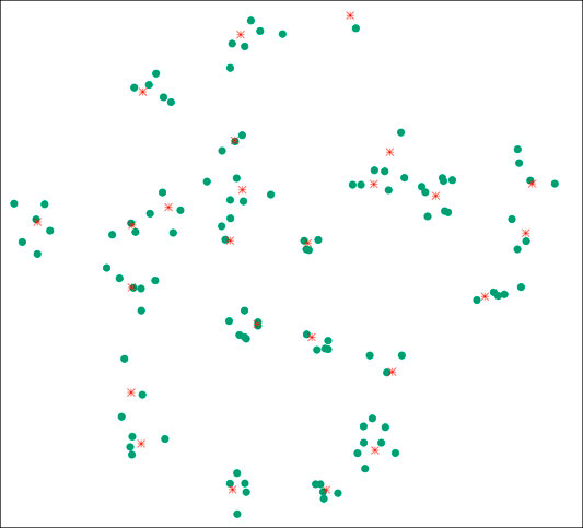
FIGURE 1. A sample of a 2-dimensional cluster point process ( represents the points of the cluster point process and represents the points of the parent process).

3.1 Poisson-Poisson Cluster Processes

Let $\mathrm{\Phi }={\sum }_{n=1}^{\infty }{\delta }_{X_n}$ denote a homogeneous PPP on ${\mathbb{R}}^d$, which works as the parent process, and let ${\mathrm{\Psi }}_n={\sum }_{k=1}^{{\kappa }_n}{\delta }_{Y_{n,k}}$, $n\in \mathbb{N}$, denote a family of finite (therefore inhomogeneous) and mutually independent PPPs on ${\mathbb{R}}^d$, which are also independent of Φ and work as the offspring processes. Then, PPCP $\mathrm{\Psi }={\sum }_{m=1}^{\infty }{\delta }_{Y_m}$ is given as

$\mathrm{\Psi }=\sum _{n=1}^{\infty }{S}_{-X_n}{\mathrm{\Psi }}_n=\sum _{n=1}^{\infty }\sum _{k=1}^{{\kappa }_n}{\delta }_{X_n+Y_{n,k}}.(3)$

The PPCP Ψ constructed as above is stationary since the parent process Φ is stationary and the offspring processes Ψ_n, $n\in \mathbb{N}$, are independent and identically distributed [see, e.g., (Baccelli et al., 2020, Example 2.3.18)]. We assume that Φ has a positive and finite intensity λ_Φ, and Ψ_n, $n\in \mathbb{N}$, have an identical intensity measure Λ_o = μ Q, where μ is a positive constant and Q is a probability distribution on $({\mathbb{R}}^d,\mathcal{B}({\mathbb{R}}^d))$. Thus, the number of points in each offspring process follows a Poisson distribution with mean μ, so that the intensity of Ψ is equal to λ_Ψ = λ_Φμ, and offspring points are scattered on ${\mathbb{R}}^d$ according to Q independently of each other. We further assume that Q is diffuse; that is, Q({x}) = 0 for any $x\in {\mathbb{R}}^d$, to make Ψ simple. We refer to $S_{-X_n}{\mathrm{\Psi }}_n$ in (Eq. 3) as the cluster associated with X_n for $n\in \mathbb{N}$. Two main examples of the PPCPs are the (modified) Thomas point process and the Matérn cluster process [see, e.g., (Chiu et al., 2013, Example 5.5)]. When Q is an isotropic normal distribution, then the obtained PPCP is called the Thomas point process. On the other hand, when Q is the uniform distribution on a fixed ball centered at the origin, then the result is called the Matérn cluster process. Note that the PPCP Ψ and its parent process Φ fulfill the conditions of Theorem 1.

3.2 Characterization of Palm Distribution

For a stationary point process Ψ, let Ψ^!≔Ψ − δ₀ on the event {Ψ({0}) = 1}, which is referred to as the reduced Palm version of Ψ.

Lemma 1. For the stationary PPCP Ψ described in Section 3.1, the intensity measure of the reduced Palm version Ψ^! (with respect to the Palm distribution) is given by

${\mathrm{\Lambda }}_{\mathrm{\Psi }}^0\left(B\right)≔{\mathbb{E}}_{\mathrm{\Psi }}^0\left[{\mathrm{\Psi }}^{!}\left(B\right)\right]={\lambda }_{\mathrm{\Phi }}\mu |B|+\mu {\int }_{{\mathbb{R}}^d}Q\left(B-y\right)Q^{-}\left(\mathrm{d}y\right),B\in \mathcal{B}\left({\mathbb{R}}^d\right),(4)$

where |⋅| denotes the Lebesgue measure on $({\mathbb{R}}^d,\mathcal{B}({\mathbb{R}}^d))$ and Q⁻(B) = Q(−B) with − B = { − x: x ∈ B} for $B\in \mathcal{B}({\mathbb{R}}^d)$.

Proof. Since the offspring processes Ψ_n, $n\in \mathbb{N}$, are PPPs, the PPCP Ψ is a Cox point process; that is, once the parent process $\mathrm{\Phi }={\sum }_{n=1}^{\infty }{\delta }_{X_n}$ is given, Ψ is conditionally an inhomogeneous PPP with a conditional intensity measure $\mu {\sum }_{n=1}^{\infty }{S}_{-X_n}Q$ [see, e.g., (Baccelli et al., 2020, Example 2.3.13)]. Since the reduced Palm version of a PPP is identical in distribution to its original version (not conditioned on {Ψ({0}) = 1}) by Slivnyak’s theorem [see, e.g., (Daley and Vere-Jones, 2008, Proposition 13.1.VII) or (Baccelli et al., 2020, Theorem 3.2.4)], we have

${\mathbb{E}}_{\mathrm{\Psi }}^0\left[{\mathrm{\Psi }}^{!}\left(B\right)\mid \mathrm{\Phi }\right]=\mathbb{E}\left[\mathrm{\Psi }\left(B\right)\mid \mathrm{\Phi }\right]=\mu \sum _{n=1}^{\infty }Q\left(B-X_n\right),B\in \mathcal{B}\left({\mathbb{R}}^d\right).$

Taking the expectation with respect to ${\mathbb{P}}_{\mathrm{\Psi }}^0$ and then applying Theorem 1, we obtain

$\begin{array}{ll}\hfill {\mathbb{E}}_{\mathrm{\Psi }}^0\left[{\mathrm{\Psi }}^{!}\left(B\right)\right]& =\mu {\mathbb{E}}_{\mathrm{\Psi }}^0\left[\sum _{n=1}^{\infty }Q\left(B-X_n\right)\right]={\mathbb{E}}_{\mathrm{\Phi }}^0\left[{\int }_{{\mathbb{R}}^d}\left(\sum _{n=1}^{\infty }Q\left(B-X_n\right)\right)◦{\theta }_y{\mathrm{\Psi }}_0\left(\mathrm{d}y\right)\right]\hfill \\ \hfill & ={\mathbb{E}}_{\mathrm{\Phi }}^0\left[{\int }_{{\mathbb{R}}^d}\sum _{n=0}^{\infty }Q\left(B-X_n+y\right){\mathrm{\Psi }}_0\left(\mathrm{d}y\right)\right]\hfill \\ \hfill & =\mu {\int }_{{\mathbb{R}}^d}\left(Q\left(B+y\right)+{\mathbb{E}}_{\mathrm{\Phi }}^0\left[\sum _{n=1}^{\infty }Q\left(B-X_n+y\right)\right]\right)Q\left(\mathrm{d}y\right),\hfill \end{array}$

where λ_Ψ = λ_Φμ is used in the second equality, the third equality follows because, for any $n\in \mathbb{N}$ and $y\in {\mathbb{R}}^d$, there exists an $n^{\prime }\in \mathbb{N}\cup \{0\}$ such that X_n◦θ_y = X_n’ − y on {Φ({0}) = 1}, and in the last equality, we apply Campbell’s formula [see, e.g., (Last and Penrose, 2017, Proposition 2.7) or (Baccelli et al., 2020, Theorem 1.2.5)] for Ψ₀. For the expectation in the last expression above, Slivnyak’s theorem, Campbell’s formula for Φ and then Fubini’s theorem yield

$\begin{array}{ll}\hfill {\mathbb{E}}_{\mathrm{\Phi }}^0\left[\sum _{n=1}^{\infty }Q\left(B-X_n+y\right)\right]& ={\lambda }_{\mathrm{\Phi }}{\int }_{{\mathbb{R}}^d}Q\left(B-x\right)\mathrm{d}x={\lambda }_{\mathrm{\Phi }}{\int }_{{\mathbb{R}}^d}{\int }_{B-x}Q\left(\mathrm{d}z\right)\mathrm{d}x\hfill \\ \hfill & ={\lambda }_{\mathrm{\Phi }}{\int }_{{\mathbb{R}}^d}{\int }_{B-z}\mathrm{d}xQ\left(\mathrm{d}z\right)={\lambda }_{\mathrm{\Phi }}|B|,\hfill \end{array}$

which completes the proof.

Remark 2. The second term on the right-hand side of (Eq. 4) is of course equal to μ∫Q(B + y) Q(dy). We adopt the form in Lemma 1 due to its interpretability. Since Q is the distribution for the position of an offspring point viewed from its parent, Q⁻ represents the distribution for the location of the parent of the offspring point at the origin on the event {Ψ({0}) = 1}. On the other hand, μ Q(B − y) gives the expected number of offspring points falling in $B\in \mathcal{B}({\mathbb{R}}^d)$ among a cluster whose parent is shifted to $y\in {\mathbb{R}}^d$. In other words, the second term on the right-hand side of (Eq. 4) represents the expected number of offspring points falling in B among the cluster which is given to have one point at the origin. Since the first term on the right-hand side of (Eq. 4) is equal to ${\mathrm{\Lambda }}_{\mathrm{\Psi }}(B)=\mathbb{E}[\mathrm{\Psi }(B)]$, Lemma 1 states that the intensity measure for the reduced Palm version of a stationary PPCP is given as the sum of the intensity measure of the stationary version and that of a cluster which has one point at the origin. Lemma 1 is also a slight generalization of the result in (Tanaka et al., 2008, Section 2.2).The observation in Remark 2 is further enhanced by the following proposition.

Proposition 1. For the stationary PPCP $\mathrm{\Psi }={\sum }_{m=1}^{\infty }{\delta }_{Y_m}$ described in Section 3.1, the generating functional of the reduced Palm version Ψ^! (with respect to the Palm distribution) is given by

${\mathcal{G}}_{\mathrm{\Psi }}^0\left(h\right)≔{\mathbb{E}}_{\mathrm{\Psi }}^0\left[\prod _{m=1}^{\infty }h\left(Y_m\right)\right]={\mathcal{G}}_{\mathrm{\Psi }}\left(h\right){\int }_{{\mathbb{R}}^d}\tilde{h}\left(z\right)Q^{-}\left(\mathrm{d}z\right),(5)$

for any measurable function h: ${\mathbb{R}}^d\to [\mathrm{0,1}]$, where ${\mathcal{G}}_{\mathrm{\Psi }}$ is the generating functional of the stationary version of Ψ given as

${\mathcal{G}}_{\mathrm{\Psi }}\left(h\right)≔\mathbb{E}\left[\sum _{m=1}^{\infty }h\left(Y_m\right)\right]={\mathcal{G}}_{\mathrm{\Phi }}\left(\tilde{h}\right)=\exp \left(-{\lambda }_{\mathrm{\Phi }}{\int }_{{\mathbb{R}}^d}\left[1-\tilde{h}\left(x\right)\right]\mathrm{d}x\right),(6)$

and $\tilde{h}(x)$ denotes the generating functional of an offspring process Ψ₁ whose parent is shifted to $x\in {\mathbb{R}}^d$;

$\tilde{h}\left(x\right)={\mathcal{G}}_{{\mathrm{\Psi }}_1}\left(S_{x}h\right)=\exp \left(-\mu {\int }_{{\mathbb{R}}^d}\left[1-h\left(x+y\right)\right]Q\left(\mathrm{d}y\right)\right).(7)$

Note that in Proposition 1 above, ${\mathcal{G}}_{\mathrm{\Phi }}$ is the generating functional of the parent process Φ. The relation ${\mathcal{G}}_{\mathrm{\Psi }}(h)={\mathcal{G}}_{\mathrm{\Phi }}(\tilde{h})$ with $\tilde{h}(x)={\mathcal{G}}_{{\mathrm{\Psi }}_1}(S_{x}h)$ in Eqs 6, 7 is known to hold for more general cluster point processes [see, e.g., (Daley and Vere-Jones, 2003, Example 6.3(a)] or [Baccelli et al., 2020, Proposition 2.3.12 and Lemma 2.3.20)], whereas the last equalities in Eqs 6, 7 follow because Φ and Ψ₁ are PPPs, respectively (see, e.g., (Last and Penrose, 2017, Exercise 3.6), or [Baccelli et al., 2020, Corollary 2.1.5)]. The relation (Eq. 5) is derived in (Ganti and Haenggi, 2009, Lemma 1), to which we give another proof using the exchange formula in Theorem 1.

Proof. As stated in the proof of Lemma 1, once the parent process $\mathrm{\Phi }={\sum }_{n=1}^{\infty }{\delta }_{X_n}$ is given, the PPCP Ψ is conditionally an inhomogeneous PPP with the conditional intensity measure $\mu {\sum }_{n=1}^{\infty }{S}_{-X_n}Q$. Since the reduced Palm version of a PPP is identical in distribution to its original (not conditioned) version, we have

$\begin{array}{ll}\hfill {\mathbb{E}}_{\mathrm{\Psi }}^0\left[\prod _{m=1}^{\infty }\left.h\left(Y_m\right)\right|\mathrm{\Phi }\right]& =\mathbb{E}\left[\prod _{m=1}^{\infty }\left.h\left(Y_m\right)\right|\mathrm{\Phi }\right]\hfill \\ \hfill & =\exp \left(-\mu \sum _{n=1}^{\infty }{\int }_{{\mathbb{R}}^d}\left(1-h\left(y\right)\right)Q\left(\mathrm{d}y-X_n\right)\right)=\prod _{n=1}^{\infty }\tilde{h}\left(X_n\right),\hfill \end{array}$

where the generating functional of a PPP is applied in the second equality. Taking the expectation with respect to ${\mathbb{P}}_{\mathrm{\Psi }}^0$ and then applying Theorem 1, we obtain

$\begin{array}{ll}\hfill {\mathcal{G}}_{\mathrm{\Psi }}^0\left(h\right)& ={\mathbb{E}}_{\mathrm{\Psi }}^0\left[\prod _{n=1}^{\infty }\tilde{h}\left(X_n\right)\right]=\frac{1}{\mu }{\mathbb{E}}_{\mathrm{\Phi }}^0\left[{\int }_{{\mathbb{R}}^d}\prod _{n=0}^{\infty }\tilde{h}\left(X_n-z\right){\mathrm{\Psi }}_0\left(\mathrm{d}z\right)\right]\hfill \\ \hfill & ={\int }_{{\mathbb{R}}^d}\tilde{h}\left(-z\right){\mathbb{E}}_{\mathrm{\Phi }}^0\left[\prod _{n=1}^{\infty }\tilde{h}\left(X_n-z\right)\right]Q\left(\mathrm{d}z\right),\hfill \end{array}$

where Campbell’s formula for Ψ₀ is applied in the last equality. By Slivnyak’s theorem and the stationarity for Φ, we have ${\mathbb{E}}_{\mathrm{\Phi }}^0\left[{\prod }_{n=1}^{\infty }\tilde{h}(X_n-z)\right]=\mathbb{E}\left[{\prod }_{n=1}^{\infty }\tilde{h}(X_n)\right]={\mathcal{G}}_{\mathrm{\Phi }}(\tilde{h})$, which completes the proof.

Remark 3. The right-hand side of (Eq. 5) is given as the generating functional ${\mathcal{G}}_{\mathrm{\Psi }}(h)$ of the stationary version of Ψ multiplied by the integral term $\int \tilde{h}(z)Q^{-}(\mathrm{d}z)$. Since $\tilde{h}(z)$ represents the generating functional of an offspring process whose parent is shifted to $z\in {\mathbb{R}}^d$ and Q⁻ is the distribution of the location of the parent point of the offspring at the origin on the event {Ψ({0}) = 1}, this integral term represents the generating functional of the cluster which is given to have a point at the origin. In other words, Proposition 1 implies that, for a stationary PPCP, its Palm version is obtained by the superposition of the original stationary version and an additional independent offspring process whose parent is placed such that it has an offspring point at the origin. This observation is already found in, e.g., (Saha et al., 2019) and is also interpreted such that a point $z\in {\mathbb{R}}^d$ is first sampled from the distribution Q⁻ and the Palm version of Φ at z is then obtained as Φ + δ_z by Slivnyak’s theorem, which works as a parent process of the Palm version of Ψ. Proposition 1 indeed supports this interpretation.

3.3 Nearest-Neighbor Distance Distributions

For a stationary point process Ψ on ${\mathbb{R}}^d$, let ${\mathrm{\Psi }}^{!}={\sum }_{m=1}^{\infty }{\delta }_{Y_m}$ be its reduced Palm version on {Ψ({0}) = 1} and let Y_* denote the nearest point of Ψ^! from the origin. Then, the nearest-neighbor distance distribution for Ψ is defined as the probability distribution for ‖Y_*‖ with respect to ${\mathbb{P}}_{\mathrm{\Psi }}^0$, where ‖ ⋅‖ denotes the Euclidean distance. We show below that the nearest-neighbor distance distribution for a stationary PPCP is obtained in a similar way to Proposition 1.

Proposition 2. For the stationary PPCP Ψ described in Section 3.1, the complementary nearest-neighbor distance distribution is given by

${\mathbb{P}}_{\mathrm{\Psi }}^0\left(\Vert Y_{\ast }\Vert >r\right)={\mathcal{G}}_{\mathrm{\Phi }}\left(h_r^{*}\right)\int h_r^{\ast }\left(t\right)Q^{-}\left(\mathrm{d}t\right),r\ge 0,(8)$

where $h_r^{\ast }(x)=e^{-\mu Q(b_0(r)-x)}$ and b₀(r) denotes a d-dimensional ball centered at the origin with radius r.

Proof. As with the proof of Proposition 1, we consider the conditional probability given the parent process $\mathrm{\Phi }={\sum }_{n=1}^{\infty }{\delta }_{X_n}$ and obtain

$\begin{array}{ll}\hfill {\mathbb{P}}_{\mathrm{\Psi }}^0\left(\Vert Y_{*}\Vert >r\mid \mathrm{\Phi }\right)& ={\mathbb{P}}_{\mathrm{\Psi }}^0\left({\mathrm{\Psi }}^{!}\left(b_0\left(r\right)\right)=0\mid \mathrm{\Phi }\right)=\mathbb{P}\left(\mathrm{\Psi }\left(b_0\left(r\right)\right)=0\mid \mathrm{\Phi }\right)\hfill \\ \hfill & =\prod _{n=1}^{\infty }{e}^{-\mu Q\left(b_0\left(r\right)-X_n\right)}=\prod _{n=1}^{\infty }{h}_r^{\ast }\left(X_n\right),\hfill \end{array}(9)$

where the second equality follows from Slivnyak’s theorem and the third does because Ψ^! is conditionally an inhomogeneous PPP with the intensity measure $\mu {\sum }_{n=1}^{\infty }{S}_{-X_n}Q$ when Φ is given. The rest of the proof is similar to that of Proposition 1.

Remark 4. In (Eq. 8), the term ${\mathcal{G}}_{\mathrm{\Phi }}(h_r^{*})$ is the complementary contact distance distribution and that is obtained by taking the expectation of (Eq. 9) with respect to $\mathbb{P}$, instead of ${\mathbb{P}}_{\mathrm{\Psi }}^0$ [see, e.g., (Miyoshi, 2019)]. The result of Proposition 2 is consistent with the existing ones in, e.g., (Baudin, 1981; Afshang et al., 2017a,b; Pandey et al., 2020) and gives a unified approach to derive the nearest-neighbor distance distributions for stationary PPCPs.

4 Applications to Wireless Networks With Hotspot Clusters

In this section, we apply Theorem 1 to the analysis of a D2D network with hotspot clusters modeled using a stationary PPCP. We here suppose d = 2, but unless otherwise specified, the discussion holds for d ≥ 2 theoretically.

4.1 Model of a Device-To-Device Network

Wireless devices are distributed on ${\mathbb{R}}^d$ according to a stationary point process $\mathrm{\Psi }={\sum }_{m=1}^{\infty }{\delta }_{Y_m}$. At each time slot, each device is in transmission mode with probability p ∈ (0, 1) or in receiving mode with probability 1 − p independently of the others (half duplex with random access). Devices in the transmission mode transmit signals but can not receive ones, whereas the devices in the receiving mode can receive signals but can not transmit ones. We assume that all transmitting devices transmit signals with identical transmission power (normalized to one) and share a common frequency spectrum. The path-loss function representing attenuation of signals with distance is given by ℓ satisfying ℓ(r) ≥ 0, r > 0, and ${\int }_{ϵ}^{\infty }\ell (r)r^{d-1}\mathrm{d}r<\infty$ for ϵ > 0. We further assume that all wireless links receive Rayleigh fading effects while we ignore shadowing effects. We focus on the device at the origin, referred to as the typical device, under the condition of {Ψ({0}) = 1} and examine whether the typical device can decode messages from other transmitting devices. Let ${\mathrm{\Psi }}_{\mathsf{T}\mathsf{x}}={\sum }_{m=1}^{\infty }{\delta }_{Y_m^{\prime }}$ denote the sub-process of Ψ representing the locations of devices in the transmission mode and for each $m\in \mathbb{N}$, let H_m denote a random variable representing the fading effect on signals transmitted from the device at $Y_m^{\prime }$, where H_m, $m\in \mathbb{N}$, are mutually independent, independent of ${\mathrm{\Psi }}_{\mathsf{T}\mathsf{x}}$ and exponentially distributed with unit mean due to the Rayleigh fading. With this setup, the received signal power by the typical device amounts to $H_m\ell \Vert Y^{\prime }\_m\Vert$ when it receives signals from the device at $Y_m^{\prime }$. Hence, if the typical device is in the receiving mode and communicates with the transmitting device at $Y_m^{\prime }$, the signal-to-interference-plus-noise ratio (SINR) is given as

${\mathsf{S}\mathsf{I}\mathsf{N}\mathsf{R}}_m=\frac{H_m\ell \left(\Vert Y_m^{\prime }\Vert \right)}{\sum _{\begin{array}{c}j=1\\ j\ne m\end{array}}^{\infty }{H}_j\ell \left(\Vert Y_j^{\prime }\Vert \right)+N},(10)$

where N denotes a constant representing noise at the origin. We suppose that the typical device can successfully decode a message from the device at $Y_m^{\prime }$ if the typical device is in the receiving mode and ${\mathsf{S}\mathsf{I}\mathsf{N}\mathsf{R}}_m$ in (Eq. 10) exceeds a predefined threshold θ > 0.

4.2 Coverage Analysis

We here suppose that a device in the receiving mode communicates with the nearest device in transmission mode. The probability that the typical device can successfully decode a message from its partner is called the coverage probability and is given by

$\mathsf{C}\mathsf{P}\left(\theta \right)=\left(1-p\right)\sum _{m=1}^{\infty }{\mathbb{P}}_{\mathrm{\Psi }}^0\left({\mathsf{S}\mathsf{I}\mathsf{N}\mathsf{R}}_m>\theta ,\Vert Y_m^{\prime }\Vert \le \Vert Y_j^{\prime }\Vert ,j\in \mathbb{N}\right),(11)$

where 1 − p on the right-hand side indicates that the typical device must be in the receiving mode and the sum over $m\in \mathbb{N}$ represents the probability that the SINR from the nearest transmitting device exceeds the threshold θ. We now suppose that the point process Ψ representing the locations of devices is given as a stationary PPCP studied in Section 3. Then, ${\mathrm{\Psi }}_{\mathsf{T}\mathsf{x}}={\sum }_{m=1}^{\infty }{\delta }_{Y_m^{\prime }}$ representing the locations of devices in the transmission mode is also a stationary PPCP, where the parent process remains the same as the homogeneous PPP Φ with intensity λ_Φ, whereas the offspring processes ${\mathrm{\Psi }}_n^{\prime }={\sum }_{k=1}^{{\kappa }_n^{\prime }}{\delta }_{Y_{n,k}^{\prime }}$, $n\in \mathbb{N}$, are finite PPPs with the intensity measure pμQ.

Theorem 2. For the model of a D2D network described in Section 4.1 with the devices deployed according to a stationary PPCP in Section 3.1, the coverage probability is given by

$\mathsf{C}\mathsf{P}\left(\theta \right)=\left(1-p\right)p\mu {\int }_{{\mathbb{R}}^d}\left(I_{1,\theta }\left(t\right)+I_{2,\theta }\left(t\right)\right)Q^{-}\left(\mathrm{d}t\right),(12)$

where Q⁻ is given in Lemma 1 and

$\begin{array}{ll}\hfill I_{1,\theta }\left(t\right)& ={\int }_{{\mathbb{R}}^d}{e}^{-\theta N/\ell \left(\Vert y\Vert \right)}{C}_{\theta }\left(y,t\right)E_{\theta }\left(y\right)Q\left(\mathrm{d}y-t\right),\hfill \\ \hfill I_{2,\theta }\left(t\right)& ={\lambda }_{\mathrm{\Phi }}{\int }_{{\mathbb{R}}^d}{\int }_{{\mathbb{R}}^d}{e}^{-\theta N/\ell \left(\Vert y\Vert \right)}{C}_{\theta }\left(y,t\right)C_{\theta }\left(y,x\right)E_{\theta }\left(y\right)Q\left(\mathrm{d}y-x\right)\mathrm{d}x,\hfill \\ \hfill E_{\theta }\left(y\right)& =\exp \left(-{\lambda }_{\mathrm{\Phi }}{\int }_{{\mathbb{R}}^d}\left[1-C_{\theta }\left(y,w\right)\right]\mathrm{d}w\right),\hfill \\ \hfill C_{\theta }\left(y,x\right)& =\exp \left(-p\mu \left[1-{\int }_{\Vert z\Vert >\Vert y\Vert }{\left(1+\theta \frac{\ell \left(\Vert z\Vert \right)}{\ell \left(\Vert y\Vert \right)}\right)}^{-1}Q\left(\mathrm{d}z-x\right)\right]\right).\hfill \end{array}(13)$

Before proceeding on the proof of Theorem 2, we give an intuitive interpretation to the result of it. First, as stated in the preceding section, Q⁻ denotes the distribution for the location of the parent point of the typical device at the origin. Thus, pμI_1,θ(t) and pμI_2,θ(t) in (Eq. 12) represent the cases where the typical device, whose parent is located at $t\in {\mathbb{R}}^d$, communicates with the transmitting device in the same cluster and in a different cluster, respectively; that is, the location of the communication partner is sampled from a finite PPP with the intensity measure pμQ(dy − t) in I_1,θ(t) and is from one with pμQ(dy − x) in I_2,θ(t), where x is also sampled from a homogeneous PPP with intensity λ_Φ. Moreover, E_θ(y) represents the effect from other clusters which are neither the one having the typical device nor the one having its communication partner at y. Finally, C_θ(y, x) represents the effect of the cluster with the parent point at $x\in {\mathbb{R}}^d$ when the typical device communicates with the transmitting device at y.

Proof. Similar to the proof of Proposition 1, once the parent process $\mathrm{\Phi }={\sum }_{n=1}^{\infty }{\delta }_{X_n}$ is given, the point process ${\mathrm{\Psi }}_{\mathsf{T}\mathsf{x}}$ representing the locations of devices in the transmission mode is conditionally an inhomogeneous PPP with the conditional intensity measure $p\mu {\sum }_{n=1}^{\infty }{S}_{-X_n}Q$. Thus, we can use the corresponding approach to that obtaining the coverage probability for a cellular network with BSs deployed according to a PPP [see, e.g., (Andrews et al., 2011) or (Błaszczyszyn et al., 2018, Section 5.2)]. Since H_m, $m\in \mathbb{N}$, are mutually independent, exponentially distributed, and also independent of Φ, we have from (Eq. 11),

$\begin{array}{ll}\hfill & \left.{\mathbb{P}}_{\mathrm{\Psi }}^0\left({\mathsf{S}\mathsf{I}\mathsf{N}\mathsf{R}}_m>\theta ,\Vert Y_m^{\prime }\Vert \le \Vert Y_j^{\prime }\Vert ,j\in \mathbb{N}\right|\mathrm{\Phi }\right)\hfill \\ \hfill & ={\mathbb{P}}_{\mathrm{\Psi }}^0\left(H_m>\frac{\theta }{\ell \left(\Vert Y_m^{\prime }\Vert \right)}\left.\left(\sum _{\begin{array}{c}j=1\\ j\ne m\end{array}}^{\infty }{H}_j\ell \left(\Vert Y_j^{\prime }\Vert \right)+N\right),\Vert Y_m^{\prime }\Vert \le \Vert Y_j^{\prime }\Vert ,j\in \mathbb{N}\right|\mathrm{\Phi }\right)\hfill \\ \hfill & \left.={\mathbb{E}}_{\mathrm{\Psi }}^0\left[e^{-\theta N/\ell \left(\Vert Y_m^{\prime }\Vert \right)}\prod _{\begin{array}{c}j=1\\ j\ne m\end{array}}^{\infty }{\left(1+\theta \frac{\ell \left(\Vert Y_j^{\prime }\Vert \right)}{\ell \left(\Vert Y_m^{\prime }\Vert \right)}\right)}^{-1}{\mathbf{1}}_{\left\{\Vert Y_j^{\prime }\Vert >\Vert Y_m^{\prime }\Vert \right\}}\right|\mathrm{\Phi }\right],\hfill \end{array}$

where 1_A denotes the indicator function for set A and we use $\mathbb{P}(H_m>a)=e^{-a}$ for a ≥ 0 and $\mathbb{E}[e^{-s{H}_j}]={(1+s)}^{-1}$ in the last equality. Summing the above expression over $m\in \mathbb{N}$, we have from Slivnyak’s Theorem for Ψ conditioned on Φ and the refined Campbell formula [see, e.g., (Daley and Vere-Jones, 2008, Theorem 13.2. III), (Last and Penrose, 2017, Theorem 9.1) or (Baccelli et al., 2020, Theorem 3.1.9)],

$\begin{array}{ll}\hfill & \left.\sum _{m=1}^{\infty }{\mathbb{P}}_{\mathrm{\Psi }}^0\left({\mathsf{S}\mathsf{I}\mathsf{N}\mathsf{R}}_m>\theta ,\Vert Y_m^{\prime }\Vert \le \Vert Y_j^{\prime }\Vert ,j\in \mathbb{N}\right|\mathrm{\Phi }\right)\hfill \\ \hfill & \left.=p\mu \sum _{n=1}^{\infty }{\int }_{{\mathbb{R}}^d}{e}^{-\theta N/\ell \left(\Vert y\Vert \right)}\mathbb{E}\left[\prod _{j=1}^{\infty }{\left(1+\theta \frac{\ell \left(\Vert Y_j^{\prime }\Vert \right)}{\ell \left(\Vert y\Vert \right)}\right)}^{-1}{\mathbf{1}}_{\left\{\Vert Y_j^{\prime }\Vert >\Vert y\Vert \right\}}\right|\mathrm{\Phi }\right]Q\left(\mathrm{d}y-X_n\right).\hfill \end{array}(14)$

Furthermore, the generating functional of a PPP applying to the above expectation yields

$\begin{array}{ll}\hfill & \left.\mathbb{E}\left[\prod _{j=1}^{\infty }{\left(1+\theta \frac{\ell \left(\Vert Y_j^{\prime }\Vert \right)}{\ell \left(\Vert y\Vert \right)}\right)}^{-1}{\mathbf{1}}_{\left\{\Vert Y_j^{\prime }\Vert >\Vert y\Vert \right\}}\right|\mathrm{\Phi }\right]\hfill \\ \hfill & =\exp \left(-p\mu \sum _{i=1}^{\infty }{\int }_{{\mathbb{R}}^d}\left[1-{\left(1+\theta \frac{\ell \left(\Vert z\Vert \right)}{\ell \left(\Vert y\Vert \right)}\right)}^{-1}{\mathbf{1}}_{\left\{\Vert z\Vert >\Vert y\Vert \right\}}\right]Q\left(\mathrm{d}z-X_i\right)\right)\hfill \\ \hfill & =\prod _{i=1}^{\infty }\exp \left(-p\mu \left[1-{\int }_{\Vert z\Vert >\Vert y\Vert }{\left(1+\theta \frac{\ell \left(\Vert z\Vert \right)}{\ell \left(\Vert y\Vert \right)}\right)}^{-1}Q\left(\mathrm{d}z-X_i\right)\right]\right)=\prod _{i=1}^{\infty }{C}_{\theta }\left(y,X_i\right).\hfill \end{array}$

Plugging this into (Eq. 14), taking the expectation with respect to ${\mathbb{P}}_{\mathrm{\Psi }}^0$ and then applying Neveu’s exchange formula in Theorem 1, we have

$\begin{array}{ll}\hfill \mathsf{C}\mathsf{P}\left(\theta \right)& =\left(1-p\right)p\mu {\mathbb{E}}_{\mathrm{\Psi }}^0\left[\sum _{n=1}^{\infty }{\int }_{{\mathbb{R}}^d}{e}^{-\theta N/\ell \left(\Vert y\Vert \right)}\prod _{i=1}^{\infty }{C}_{\theta }\left(y,X_i\right)Q\left(\mathrm{d}y-X_n\right)\right]\hfill \\ \hfill & =\left(1-p\right)p{\mathbb{E}}_{\mathrm{\Phi }}^0\left[{\int }_{{\mathbb{R}}^d}\sum _{n=0}^{\infty }{\int }_{{\mathbb{R}}^d}{e}^{-\theta N/\ell \left(\Vert y\Vert \right)}\prod _{i=0}^{\infty }{C}_{\theta }\left(y,X_i-t\right)Q\left(\mathrm{d}y-X_n+t\right){\mathrm{\Psi }}_0\left(\mathrm{d}t\right)\right]\hfill \\ \hfill & =\left(1-p\right)p\mu {\int }_{{\mathbb{R}}^d}{\mathbb{E}}_{\mathrm{\Phi }}^0\left[\sum _{n=0}^{\infty }{\int }_{{\mathbb{R}}^d}{e}^{-\theta N/\ell \left(\Vert y\Vert \right)}\prod _{i=0}^{\infty }{C}_{\theta }\left(y,X_i-t\right)Q\left(\mathrm{d}y-X_n+t\right)\right]Q\left(\mathrm{d}t\right),\hfill \end{array}(15)$

where we note the existence of X₀ = 0 on {Φ({0}) = 1} in the second equality and apply Campbell’s formula in the third equality. Noting that X₀ = 0 on {Φ({0}) = 1}, we separate the expectation in (Eq. 15) into

$\begin{array}{ll}\hfill & {\mathbb{E}}_{\mathrm{\Phi }}^0\left[\sum _{n=0}^{\infty }{\int }_{{\mathbb{R}}^d}{e}^{-\theta N/\ell \left(\Vert y\Vert \right)}\prod _{i=0}^{\infty }{C}_{\theta }\left(y,X_i-t\right)Q\left(\mathrm{d}y-X_n+t\right)\right]\hfill \\ \hfill & ={\int }_{{\mathbb{R}}^d}{e}^{-\theta N/\ell \left(\Vert y\Vert \right)}{C}_{\theta }\left(y,-t\right){\mathbb{E}}_{\mathrm{\Phi }}^0\left[\prod _{i=1}^{\infty }{C}_{\theta }\left(y,X_i-t\right)\right]Q\left(\mathrm{d}y+t\right)\hfill \\ \hfill & +{\mathbb{E}}_{\mathrm{\Phi }}^0\left[\sum _{n=1}^{\infty }{\int }_{{\mathbb{R}}^d}{e}^{-\theta N/\ell \left(\Vert y\Vert \right)}{C}_{\theta }\left(y,-t\right)C_{\theta }\left(y,X_n-t\right)\prod _{\begin{array}{c}i=1\\ i\ne n\end{array}}^{\infty }{C}_{\theta }\left(y,X_i-t\right)Q\left(\mathrm{d}y-X_n+t\right)\right],\hfill \end{array}(16)$

and consider the two terms on the right-hand side of (Eq. 16) one by one. For the first term, the generating functional of a PPP yields (1st term of (Eq. 16))

$\begin{array}{ll}\hfill & ={\int }_{{\mathbb{R}}^d}{e}^{-\theta N/\ell \left(\Vert y\Vert \right)}{C}_{\theta }\left(y,-t\right)\exp \left(-{\lambda }_{\mathrm{\Phi }}{\int }_{{\mathbb{R}}^d}\left[1-C_{\theta }\left(y,w\right)\right]\mathrm{d}w\right)Q\left(\mathrm{d}y+t\right)\hfill \\ =I_{1,\theta }\left(-t\right).\hfill \end{array}(17)$

On the other hand, applying Campbell’s formula and the generating functional for Φ to the second term on the right-hand side of (Eq. 16), we have (2nd term of (Eq. 16))

$\begin{array}{ll}\hfill & ={\lambda }_{\mathrm{\Phi }}{\int }_{{\mathbb{R}}^d}{\int }_{{\mathbb{R}}^d}{e}^{-\theta N/\ell \left(\Vert y\Vert \right)}{C}_{\theta }\left(y,-t\right)C_{\theta }\left(y,x\right){\mathbb{E}}_{\mathrm{\Phi }}^0\left[\prod _{i=1}^{\infty }{C}_{\theta }\left(y,X_i-t\right)\right]Q\left(\mathrm{d}y-x\right)\mathrm{d}x\hfill \\ \hfill & ={\lambda }_{\mathrm{\Phi }}{\int }_{{\mathbb{R}}^d}{\int }_{{\mathbb{R}}^d}{e}^{-\theta N/\ell \left(\Vert y\Vert \right)}{C}_{\theta }\left(y,-t\right)C_{\theta }\left(y,x\right)\exp \left(-{\lambda }_{\mathrm{\Phi }}{\int }_{{\mathbb{R}}^d}\left[1-C_{\theta }\left(y,w\right)\right]\mathrm{d}w\right)Q\left(\mathrm{d}y-x\right)\mathrm{d}x\hfill \\ \hfill & =I_{2,\theta }\left(-t\right).\hfill \end{array}(18)$

Finally, plugging (Eqs 17, 18) into (Eq. 16), and then into (Eq. 15), we have (Eq. 12) and the proof is completed.When d = 2 and the distribution Q for the locations of offspring points depends only on the distance; that is, Q(dy) = f_o(‖y‖) dy for $y\in {\mathbb{R}}^2$, we obtain a numerically computable form of the coverage probability.

Corollary 1. When d = 2 and Q(dy) = f_o(‖y‖) dy, $y\in {\mathbb{R}}^2$, the coverage probability in Theorem 2 is reduced to

$\mathsf{C}\mathsf{P}\left(\theta \right)=2\pi \left(1-p\right)p\mu {\int }_0^{\infty }{\int }_0^{\infty }{e}^{-\theta N/\ell \left(s\right)}{\widehat{E}}_{\theta }\left(s\right){\widehat{C}}_{\theta }\left(s,u\right){\widehat{I}}_{\theta }\left(s,u\right)\mathrm{d}s{f}_{\mathrm{o}}\left(u\right)u\mathrm{d}u,(19)$

where

$\begin{array}{ll}\hfill {\widehat{I}}_{\theta }\left(s,u\right)& =g\left(s\mid u\right)+2\pi {\lambda }_{\mathrm{\Phi }}{\int }_0^{\infty }{\widehat{C}}_{\theta }\left(s,r\right)g\left(s\mid r\right)r\mathrm{d}r,\hfill \\ \hfill {\widehat{E}}_{\theta }\left(s\right)& =\exp \left(-2\pi {\lambda }_{\mathrm{\Phi }}{\int }_0^{\infty }\left[1-{\widehat{C}}_{\theta }\left(s,v\right)\right]v\mathrm{d}v\right),\hfill \\ \hfill {\widehat{C}}_{\theta }\left(s,r\right)& =\exp \left(-p\mu \left[1-{\int }_s^{\infty }{\left(1+\theta \frac{\ell \left(q\right)}{\ell \left(s\right)}\right)}^{-1}g\left(q\mid r\right)\mathrm{d}q\right]\right),\hfill \\ \hfill g\left(s\mid r\right)& =2s{\int }_0^{\pi }{f}_{\mathrm{o}}\left(\sqrt{s^2+r^2-2sr\cos \phi }\right)\mathrm{d}\phi .\hfill \end{array}(20)$

Proof. Since the distribution Q depends only on the distance, it holds that Q⁻(dt) = Q(dt) = f_o(‖t‖) dt, $t\in {\mathbb{R}}^2$, and (Eq. 12) is reduced to

$\begin{array}{ll}\hfill \mathsf{C}\mathsf{P}\left(\theta \right)& =\left(1-p\right)p\mu {\int }_{{\mathbb{R}}^2}\left(I_{1,\theta }\left(t\right)+I_{2,\theta }\left(t\right)\right)f_{\mathrm{o}}\left(\Vert t\Vert \right)\mathrm{d}t\hfill \\ \hfill & =2\pi \left(1-p\right)p\mu {\int }_0^{\infty }\left({\widehat{I}}_{1,\theta }\left(u\right)+{\widehat{I}}_{2,\theta }\left(u\right)\right)f_{\mathrm{o}}\left(u\right)u\mathrm{d}u,\hfill \end{array}(21)$

where the polar coordinate conversion is applied in the second equality and

$\begin{array}{ll}\hfill {\widehat{I}}_{1,\theta }\left(u\right)& ={\int }_0^{\infty }{e}^{-\theta N/\ell \left(s\right)}{\widehat{C}}_{\theta }\left(s,u\right){\widehat{E}}_{\theta }\left(s\right)g\left(s\mid u\right)\mathrm{d}s,\hfill \\ \hfill {\widehat{I}}_{2,\theta }\left(u\right)& =2\pi {\lambda }_{\mathrm{\Phi }}{\int }_0^{\infty }{\int }_0^{\infty }{e}^{-\theta N/\ell \left(s\right)}{\widehat{C}}_{\theta }\left(s,u\right){\widehat{C}}_{\theta }\left(s,r\right){\widehat{E}}_{\theta }\left(s\right)g\left(s\mid r\right)\mathrm{d}sr\mathrm{d}r.\hfill \end{array}$

Therefore, we have

${\widehat{I}}_{1,\theta }\left(u\right)+{\widehat{I}}_{2,\theta }\left(u\right)={\int }_0^{\infty }{e}^{-\theta N/\ell \left(s\right)}{\widehat{C}}_{\theta }\left(s,u\right){\widehat{E}}_{\theta }\left(s\right){\widehat{I}}_{\theta }\left(s,u\right)\mathrm{d}s.$

Plugging this into (Eq. 21), we have (Eq. 19) and the proof is completed.

4.3 Device Discovery

We next consider the problem of device discovery. Devices in the transmission mode transmit broadcast messages, whereas a device in the receiving mode can discover the transmitters if it can successfully decode the broadcast messages. When a device in the receiving mode receives the signal from one transmitting device, the signals from all other transmitting devices work as interference. Then, the expected number of transmitting devices discovered by the typical device is represented by

$\mathcal{N}\left(\theta \right)=\left(1-p\right){\mathbb{E}}_{\mathrm{\Psi }}^0\left[\sum _{m=1}^{\infty }{\mathit{1}}_{\left\{{\mathsf{S}\mathsf{I}\mathsf{N}\mathsf{R}}_m>\theta \right\}}\right].(22)$

Proposition 3. Consider the D2D network model described in Section 4.1 with the devices deployed according to a stationary PPCP given in Section 3.1. Then, the expected number $\mathcal{N}(\theta )$ of transmitting devices discovered by the typical device is obtained by (Eq. 12) in Theorem 2 replacing the integral range ‖z‖ > ‖y‖ in (Eq. 13) by ${\mathbb{R}}^d$. Moreover, when d = 2 and Q(dy) = f_o(‖y‖) dy for $y\in {\mathbb{R}}^2$, $\mathcal{N}(\theta )$ is reduced to (Eq. 19) in Corollary 1 replacing the integral range (s, ∞) in (Eq. 20) by (0, ∞).

Proof. Since ${\mathbb{E}}_{\mathrm{\Psi }}^0\left[{\sum }_{m=1}^{\infty }{\mathit{1}}_{\{{\mathsf{S}\mathsf{I}\mathsf{N}\mathsf{R}}_m>\theta \}}\right]={\sum }_{m=1}^{\infty }{\mathbb{P}}_{\mathrm{\Psi }}^0({\mathsf{S}\mathsf{I}\mathsf{N}\mathsf{R}}_m>\theta )$, the difference between (Eq. 11) and (Eq. 22) is only the event $\{\Vert Y_m^{\prime }\Vert \le \Vert Y_j^{\prime }\Vert ,j\in \mathbb{N}\}$. This leads to the difference of the integral ranges in C_θ(y, x) in (Eq. 13) and in ${\widehat{C}}_{\theta }(s,r)$ in (Eq. 20). Remark 5. Since ${\mathbb{P}}_{\mathrm{\Psi }}^0\left({\bigcup }_{m=1}^{\infty }\{{\mathsf{S}\mathsf{I}\mathsf{N}\mathsf{R}}_m>\theta \}\right)\le {\sum }_{m=1}^{\infty }{\mathbb{P}}_{\mathrm{\Psi }}^0({\mathsf{S}\mathsf{I}\mathsf{N}\mathsf{R}}_m>\theta )=\mathcal{N}(\theta )$, Proposition 3 also gives an upper bound for the coverage probability with the max-SINR association policy, where a device in the receiving mode receives a message with the strongest SINR. This upper bound is known to be exact for θ > 1 since ${\sum }_{m=1}^{\infty }{\mathit{1}}_{\{{\mathsf{S}\mathsf{I}\mathsf{N}\mathsf{R}}_m>\theta \}}\le 1+{\theta }^{-1}$ almost surely [see (Dhillon et al., 2012) or (Błaszczyszyn et al., 2018, Lemma 5.1.2)].

4.4 Numerical Experiments

We present the results of numerical experiments for the analytical results obtained in Sections 4.2, 4.3. We set d = 2 and the distribution Q for the location of the offspring points as Q(dy) = f_o(‖y‖) dy and $f_{\mathrm{o}}(s)=e^{-s^2/(2{\sigma }^2)}/(2\pi {\sigma }^2)$, s ≥ 0; that is, Q is the isotropic normal distribution with variance σ², so that the resulting PPCP Ψ is the Thomas point process. Furthermore, the path-loss function is set as ℓ(r) = r^−β, r > 0, with β > 2.

The numerical results for the coverage probability are given in Figure 2, where the values of $\mathsf{C}\mathsf{P}(\theta )$ with different values of θ and σ² are plotted. The other parameters are fixed at λ_Φ = π⁻¹, μ = 10, p = 0.5, β = 4 and N = 0. For comparison, the values when the devices are located according to a homogeneous PPP are also displayed in the figure with the label “σ² → ∞.” From Figure 2, we can see that, as the value of σ² increases, the coverage probability decreases and is closer to that for the homogeneous PPP. This is contrary to the case of cellular networks, where the coverage probability increases and is closer to that for the homogeneous PPP from below as the variance of the locations of offspring points increases [see (Miyoshi, 2019)]. This difference is thought to be due to the fact that the locations of a receiving device and its communication partner are near to each other in the PPCP-deployed D2D network since they are both points of the same PPCP, whereas the location of a receiver is likely far from that of the associated BS in the PPCP-deployed cellular network since their locations are independent of each other.

FIGURE 2

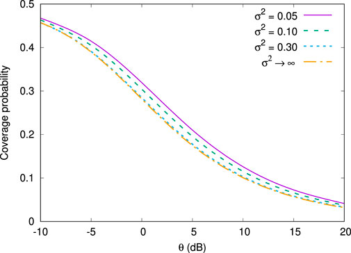
FIGURE 2. Coverage probability as a function of SINR threshold (λ_Φ = π⁻¹, μ = 10, p = 0.5, β = 4 and N = 0).

The results of the device discovery is given in Figure 3, where we know that the closed form expression of the expected number of discovered devices is obtained as ${\mathcal{N}}^{(\mathsf{P}\mathsf{P}\mathsf{P})}(\theta )=(1-p)(\beta /2\pi )\sin (2\pi /\beta ){\theta }^{-2/\beta }$ for the case of the homogeneous PPP with N ≡ 0 [see, e.g., (Hamida et al., 2008)]. The figure shows similar features to the coverage probability.

FIGURE 3

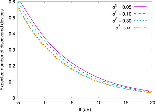
FIGURE 3. Expected number of discovered devices as a function of SINR threshold (λ_Φ = π⁻¹, μ = 10, p = 0.5, β = 4 and N = 0).

5 Conclusion

In this paper, we have presented an alternative form of Neveu’s exchange formula for jointly stationary point processes on ${\mathbb{R}}^d$ and then demonstrated that it is useful for the analysis of spatial stochastic models given based on stationary PPCPs. We have first applied it to the Palm characterization for a stationary PPCP and then to the analysis of a D2D network modeled using a stationary PPCP. Although we have only considered some fundamental problems, we expect that the new form of the exchange formula will be utilized for the analysis of more sophisticated models leading up to the development of 5G and beyond networks.

Data Availability Statement

The original contributions presented in the study are included in the article/supplementary material, further inquiries can be directed to the corresponding author.

Author Contributions

The author confirms being the sole contributor of this work and has approved it for publication.

Funding

This work was supported by the Japan Society for the Promotion of Science (JSPS) Grant-in-Aid for Scientific Research (C) 19K11838.

Conflict of Interest

The author declares that the research was conducted in the absence of any commercial or financial relationships that could be construed as a potential conflict of interest.

Publisher’s Note

All claims expressed in this article are solely those of the authors and do not necessarily represent those of their affiliated organizations, or those of the publisher, the editors and the reviewers. Any product that may be evaluated in this article, or claim that may be made by its manufacturer, is not guaranteed or endorsed by the publisher.

References

Afshang, M., Dhillon, H. S., and Chong, P. H. J. (2016). Modeling and Performance Analysis of Clustered Device-To-Device Networks. IEEE Trans. Wirel. Commun. 15, 4957–4972. doi:10.1109/twc.2016.2550024

CrossRef Full Text | Google Scholar

Afshang, M., and Dhillon, H. S. (2018). Poisson Cluster Process Based Analysis of HetNets with Correlated User and Base Station Locations. IEEE Trans. Wirel. Commun. 17, 2417–2431. doi:10.1109/twc.2018.2794983

CrossRef Full Text | Google Scholar

Afshang, M., Saha, C., and Dhillon, H. S. (2017a). Nearest-Neighbor and Contact Distance Distributions for Matérn Cluster Process. IEEE Commun. Lett. 21, 2686–2689. doi:10.1109/lcomm.2017.2747510

CrossRef Full Text | Google Scholar

Afshang, M., Saha, C., and Dhillon, H. S. (2017b). Nearest-neighbor and Contact Distance Distributions for Thomas Cluster Process. IEEE Wirel. Commun. Lett. 6, 130–133.

Google Scholar

Andrews, J. G., Gupta, A. K., and Dhillon, H. S. (2016). A Primer on Cellular Network Analysis Using Stochastic Geometry. ArXiv:1604.03183 [cs.IT]. doi:10.48550/arXiv.1604.03183

CrossRef Full Text | Google Scholar

Andrews, J. G., Baccelli, F., and Ganti, R. K. (2011). A Tractable Approach to Coverage and Rate in Cellular Networks. IEEE Trans. Commun. 59, 3122–3134. doi:10.1109/tcomm.2011.100411.100541

CrossRef Full Text | Google Scholar

Baccelli, F., Błaszczyszyn, B., and Karray, M. (2020). Random Measures, Point Processes, and Stochastic Geometry. Available at: https://hal.inria.fr/hal-02460214.

Google Scholar

Baccelli, F., and Błaszczyszyn, B. (2009a). Stochastic Geometry and Wireless Networks: Volume I Theory. FNT Netw. 3, 249–449. doi:10.1561/1300000006

CrossRef Full Text | Google Scholar

Baccelli, F., and Błaszczyszyn, B. (2009b). Stochastic Geometry and Wireless Networks: Volume II Applications. FNT Netw. 4, 1–312. doi:10.1561/1300000026

CrossRef Full Text | Google Scholar

Baccelli, F., Khud, N., Laroia, R., Li, J., Richardson, T., Shakkottai, S., et al. (2012). “On the Design of Device-To-Device Autonomous Discovery,” in 2012 Fourth International Conference on Communication Systems and Networks (Bangalore, India: COMSNETS), 1–9. doi:10.1109/comsnets.2012.6151335

CrossRef Full Text | Google Scholar

Baudin, M. (1981). Likelihood and Nearest-Neighbor Distance Properties of Multidimensional Poisson Cluster Processes. J. Appl. Probab. 18, 879–888. doi:10.2307/3213062

CrossRef Full Text | Google Scholar

Błaszczyszyn, B., Haenggi, M., Keeler, P., and Mukherjee, S. (2018). Stochastic Geometry Analysis of Cellular Networks. Cambridge: Cambridge University Press.

Google Scholar

Błaszczyszyn, B., and Yogeshwaran, D. (2009). Directionally Convex Ordering of Random Measures, Shot Noise Fields, and Some Applications to Wireless Communications. Adv. Appl. Probab. 41, 623–646.

Google Scholar

Chen, L., Wang, W., and Zhang, C. (2017). Stochastic Wireless Powered Communication Networks with Truncated Cluster Point Process. IEEE Trans. Veh. Technol. 66, 11286–11294. doi:10.1109/tvt.2017.2726003

CrossRef Full Text | Google Scholar

Chiu, S. N., Stoyan, D., Kendall, W. S., and Mecke, J. (2013). Stochastic Geometry and its Applications. 3rd edn. Wiley.

Google Scholar

Chun, Y. J., Hasna, M. O., and Ghrayeb, A. (2015). Modeling Heterogeneous Cellular Networks Interference Using Poisson Cluster Processes. IEEE J. Sel. Areas Commun. 33, 2182–2195. doi:10.1109/jsac.2015.2435271

CrossRef Full Text | Google Scholar

Daley, D. J., and Vere-Jones, D. (2003). An Introduction to the Theory of Point Processes: Volume I: Elementary Theory and Methods. 2nd edn. Switzerland: Springer.

Google Scholar

Daley, D. J., and Vere-Jones, D. (2008). An Introduction to the Theory of Point Processes: Volume II: General Theory and Structure. 2nd edn. Switzerland: Springer.

Google Scholar

Dhillon, H. S., Ganti, R. K., Baccelli, F., and Andrews, J. G. (2012). Modeling and Analysis of K-Tier Downlink Heterogeneous Cellular Networks. IEEE J. Sel. Areas Commun. 30, 550–560. doi:10.1109/jsac.2012.120405

CrossRef Full Text | Google Scholar

ElSawy, H., Sultan-Salem, A., Alouini, M.-S., and Win, M. Z. (2017). Modeling and Analysis of Cellular Networks Using Stochastic Geometry: A Tutorial. IEEE Commun. Surv. Tutorials 19, 167–203. doi:10.1109/comst.2016.2624939

CrossRef Full Text | Google Scholar

Ganti, R. K., and Haenggi, M. (2009). Interference and Outage in Clustered Wireless Ad Hoc Networks. IEEE Trans. Inf. Theory 55, 4067–4086. doi:10.1109/tit.2009.2025543

CrossRef Full Text | Google Scholar

Gentner, D., and Last, G. (2011). Palm Pairs and the General Mass-Transport Principle. Math. Z. 267, 695–716. doi:10.1007/s00209-009-0642-4

CrossRef Full Text | Google Scholar

Haenggi, M., and Ganti, R. K. (2009). Interference in Large Wireless Networks. Found. Trends Netw. 3, 127–248.

Google Scholar

Haenggi, M. (2013). Stochastic Geometry for Wireless Networks. Cambridge: Cambridge University Press.

Google Scholar

Hamida, E. B., Chelius, G., Busson, A., and Fleury, E. (2008). Neighbor Discovery in Multi-Hop Wireless Networks: Evaluation and Dimensioning with Interference Considerations. Discrete Math. Theor. Comput. Sci. 10, 87–114.

Google Scholar

Hmamouche, Y., Benjillali, M., Saoudi, S., Yanikomeroglu, H., and Renzo, M. D. (2021). New Trends in Stochastic Geometry for Wireless Networks: A Tutorial and Survey. Proc. IEEE 109, 1200–1252. doi:10.1109/jproc.2021.3061778

CrossRef Full Text | Google Scholar

Kwon, T., and Choi, J.-W. (2014). Spatial Performance Analysis and Design Principles for Wireless Peer Discovery. IEEE Trans. Wirel. Commun. 13, 4507–4519. doi:10.1109/twc.2014.2321142

CrossRef Full Text | Google Scholar

Kwon, T., Ju, H., and Lee, H. (2020). Performance Study for Random Access-Based Wireless Mutual Broadcast Networks with Ginibre Point Processes. IEEE Commun. Lett. 24, 1581–1585. doi:10.1109/lcomm.2020.2987913

CrossRef Full Text | Google Scholar

Last, G. (2010). “Modern Random Measures: Palm Theory and Related Models,” in New Perspectives in Stochastic Geometry. Editors W. S. Kendall, and I. Molchanov (United Kingdom: Oxford University Press), 77–110.

Google Scholar

Last, G., and Penrose, M. (2017). Lectures on the Poisson Process. Cambridge: Cambridge University Press.

Google Scholar

Last, G., and Thorisson, H. (2009). Invariant Transports of Stationary Random Measures and Mass-Stationarity. Ann. Probab. 37, 790–813. doi:10.1214/08-aop420

CrossRef Full Text | Google Scholar

Lu, X., Salehi, M., Haenggi, M., Hossain, E., and Jiang, H. (2021). Stochastic Geometry Analysis of Spatial-Temporal Performance in Wireless Networks: A Tutorial. IEEE Commun. Surv. Tutorials 23, 2753–2801. doi:10.1109/comst.2021.3104581

CrossRef Full Text | Google Scholar

Miyoshi, N. (2019). Downlink Coverage Probability in Cellular Networks with Poisson-Poisson Cluster Deployed Base Stations. IEEE Wirel. Commun. Lett. 8, 5–8. doi:10.1109/lwc.2018.2845377

CrossRef Full Text | Google Scholar

Miyoshi, N., and Shirai, T. (2014). A Cellular Network Model with Ginibre Configured Base Stations. Adv. Appl. Probab. 46, 832–845. doi:10.1239/aap/1409319562

CrossRef Full Text | Google Scholar

Miyoshi, N., and Shirai, T. (2016). Spatial Modeling and Analysis of Cellular Networks Using the Ginibre Point Process: A Tutorial. IEICE Trans. Commun. E99-B, 2247–2255. doi:10.1587/transcom.2016nei0001

CrossRef Full Text | Google Scholar

Mukherjee, S. (2014). Analytical Modeling of Heterogeneous Cellular Networks: Geometry, Coverage, and Capacity. Cambridge: Cambridge University Press.

Google Scholar

Pandey, K., Dhillon, H. S., and Gupta, A. K. (2020). On the Contact and Nearest-Neighbor Distance Distributions for the ${n}$ -Dimensional Matérn Cluster Process. IEEE Wirel. Commun. Lett. 9, 394–397. doi:10.1109/lwc.2019.2957221

CrossRef Full Text | Google Scholar

Saha, C., Afshang, M., and Dhillon, H. S. (2018). 3GPP-inspired HetNet Model Using Poisson Cluster Process: Sum-Product Functionals and Downlink Coverage. IEEE Trans. Commun. 66, 2219–2234. doi:10.1109/tcomm.2017.2782741

CrossRef Full Text | Google Scholar

Saha, C., Afshang, M., and Dhillon, H. S. (2017). Enriched $K$ -Tier HetNet Model to Enable the Analysis of User-Centric Small Cell Deployments. IEEE Trans. Wirel. Commun. 16, 1593–1608. doi:10.1109/twc.2017.2649495

CrossRef Full Text | Google Scholar

Saha, C., Dhillon, H. S., Miyoshi, N., and Andrews, J. G. (2019). Unified Analysis of HetNets Using Poisson Cluster Processes under Max-Power Association. IEEE Trans. Wirel. Commun. 18, 3797–3812. doi:10.1109/twc.2019.2917904

CrossRef Full Text | Google Scholar

Suryaprakash, V., Moller, J., and Fettweis, G. (2015). On the Modeling and Analysis of Heterogeneous Radio Access Networks Using a Poisson Cluster Process. IEEE Trans. Wirel. Commun. 14, 1035–1047. doi:10.1109/twc.2014.2363454

CrossRef Full Text | Google Scholar

Tanaka, U., Ogata, Y., and Stoyan, D. (2008). Parameter Estimation and Model Selection for Neyman-Scott Point Processes. Biom. J. 50, 43–57. doi:10.1002/bimj.200610339

PubMed Abstract | CrossRef Full Text | Google Scholar

Turgut, E., and Gursoy, M. C. (2018). Downlink Analysis in Unmanned Aerial Vehicle (UAV) Assisted Cellular Networks with Clustered Users. IEEE Access 6, 36313–36324. doi:10.1109/access.2018.2841655

CrossRef Full Text | Google Scholar

Yang, L., Lim, T. J., Zhao, J., and Motani, M. (2021). Modeling and Analysis of HetNets with Interference Management Using Poisson Cluster Process. IEEE Trans. Veh. Technol. 70, 12039–12054. doi:10.1109/tvt.2021.3114739

CrossRef Full Text | Google Scholar