Trainable Communication Systems Based on the Binary Neural Network

End-to-end learning of the communication system regards the transmitter, channel, and receiver as a neural network-based autoencoder. This approach enables joint optimization of both the transmitter and receiver and can learn to communicate more efficiently than model-based ones. Despite the achieved success, high complexity is the major disadvantage that hinders its further development, while low-precision compression such as one-bit quantization is an effective solution. This study proposed an autoencoder communication system composed of binary neural networks (BNNs), which is based on bit operations and has a great potential to be applied to hardware platforms with very limited computing resources such as FPGAs. Several modifications are explored to further improve the performance. Experiments showed that the proposed BNN-based system can achieve a performance similar to that of the existing neural network-based autoencoder systems while largely reducing the storage and computation complexities.

1 Introduction

An autoencoder-based communication system regards the entire physical layer, i.e., “transmitter-channel-receiver,” as an end-to-end data reconstruction task (O’Shea and Hoydis, 2017; Zhu et al., 2019; Ye et al., 2020). Specifically, the transmitter learns to encode the input data into a signal for channel transmission, while the receiver learns to restore the source data, according to the received signal. By comparing the source data and the recovered data, the model parameters of the entire neural network are trained end-to-end in a supervised learning manner. By this means, modules in the traditional transmission system can be integrated into one and optimized together, and a better overall performance can be obtained (Stark et al., 2019; Cammerer et al., 2020).

Despite the current success of autoencoder-based communication systems, one major disadvantage that hinders its implementation is the high complexity. Theoretically, the data-driven transmission technology can achieve better energy efficiency than traditional methods on dedicated hardware (Vanhoucke et al., 2011; Chen et al., 2017). However, the computation and storage complexities of current autoencoder-based communication systems are still much higher than those of traditional model-based systems. In particular, the device transmission rate is expected to increase by an order of magnitude in the future beyond the 5G or 6G eras, making the transmission system even more complex. In order to achieve miniaturization and productization, low-complexity autoencoder-based communication technologies need to be studied.

Deep learning systems can be accelerated at the hardware layer by using custom chips, at the framework layer such as compilation optimization, as well as at the algorithmic layer. Low-precision quantization is an effective way to achieve model compression and acceleration at the algorithmic level and thus reduces the computation and storage complexity (Han et al., 2015). The most extreme quantization is binary quantization, and the resulting model is called the binary neural network (BNN) (Qin et al., 2020). In BNNs, heavy floating-point multiplication and addition operations can be replaced by bitwise operations. Therefore, the BNN can greatly reduce the storage and computational complexity on the mobile end and has been widely used in tasks such as object recognition and image classification (Kung et al., 2018).

In this study, we proposed low-complexity autoencoder-based communication systems based on the BNN. Modifications are made to existing BNN techniques to further improve the performance. For example, we found that the exclusion of the shifting operation is trivial, while the scaling vector is critical for the performance. Experimental results showed that the proposed BNN-based autoencoder system can achieve similar performance to existing ones based on convolutional neural networks (CNNs) and dense networks while reducing the storage complexity to one-seventh and the computation complexity to one-fifth. This result verified the feasibility and effectiveness of the proposed BNN-based autoencoder communication systems.

2 Technical Background

2.1 Deep Learning Basic

The basic problem in communication is to find the representation of information and then recover that information at the other end. Since the coding and modulation method applied in the receiver and transmitter are so massive to optimize every block integrally in the same manner that enables the whole system to achieve overall performance improvement, a method of neural network training transmitter and receiver is proposed.

Recently, DL has become more advanced to be used in many fields, especially in communication such as in modulation (Felix et al., 2018), signal detection (Samuel et al., 2017), and channel decoding (Jiang et al., 2019). It takes advantage to learn and optimize the target system or the environment without depending on the waveform design, constellation, and reference signals. Under this circumstance, it is able to fit in nearly all the receiver and transmitter hardware and complex channels and make full use of wireless channel resources.

2.2 Autoencoder

Considering the feasibility of the autoencoder described in Hinton and Salakhutdinov (2006), the transmitter and receiver are capable of being optimized together at one end (Wu et al., 2019; Zhu et al., 2019). By assuming the channel model to be well known, the receiver and transmitter can be trained offline, and the parameters can also be determined beforehand. Furthermore, after the neural network has been trained for the simple channel, it only needs a change in parameters for the complex channel to expand the method in other situations.

2.3 Binary Neural Networks

Although the CNN saves a large amount of complexity compared to the densely connected network, there still exists a huge need to further reduce the model complexity. Facing with this urgent need, the BNN appears to be one reasonable solution. Compared to full-precision neural networks, the BNN saves a lot of memory and computation despite the binary operation of weights and activations and will greatly facilitate the model deployment on resource-constrained devices. Under these advantages, the traditional operation techniques of data could, therefore, be replaced by other methods like XNOR that in this way, it could largely save energy and reduce the computational cost. Specifically, the matrix multiplication applied in the system could be ideally replaced by the XNOR operation as follows:

$x_b\ast w_b=popcount\left(XNOR\left(x_b,w_b\right)\right),(1)$

Where W_b and x_b represent binarized weights and activations, respectively, and can be further applied in all of the parameters inside networks. Depending on the basic method on binarization, the weight and activations used in the network can be binarized as follows:

$x_b=Sign\left(x_r\right)=\left\{\begin{array}{c}+1,\mathrm{i}\mathrm{f}{x}_r\ge 0,\hfill \\ -1,\mathrm{i}\mathrm{f}{x}_r\le 0,\hfill \end{array}\right.(2)$

$w_b=\frac{\Vert W_r{\Vert }_{l1}}{n}Sign\left(w_r\right)=\left\{\begin{array}{c}+\frac{\Vert W_r{\Vert }_{l1}}{n},\mathrm{i}\mathrm{f}{w}_r\ge 0,\hfill \\ -\frac{\Vert W_r{\Vert }_{l1}}{n},\mathrm{i}\mathrm{f}{w}_r\le 0,\hfill \end{array}\right.(3)$

Where b denotes the binary value and $\frac{\Vert W_r{\Vert }_{l1}}{n}$ is the average value of absolute weights. The sign function helps in transforming weights and activations in to its binary form (Liu et al., 2020). There are various activation functions, and here, we mainly discussed tanh and elu. The tanh function lays its range between +1 and −1, which has soft saturation regions and with large positive and negative numbers as inputs, and the gradient goes to zero when the input absolute value is large, making neurons basically unable to renew. Being a zero-centered function, it could be described as follows, and its graph is shown in Figure 1.

$\tanh x=\frac{\mathit{sinh}x}{\mathit{cosh}x}=\frac{e^x-e^{-x}}{e^x+e^{-x}}.(4)$

As for the elu function, it is unsaturated in positive numbers and hardly saturated in negative numbers.

FIGURE 1

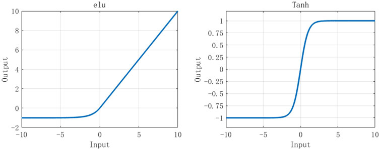
FIGURE 1. Graphs for tanh and elu.

It should be noted that elu is less computationally intensive than tanh, so it converges faster, and the output mean value is close to zero. It has negative saturation regions and is, thus, more robust to noise. It is showed in Figure 1, and its function is described as follows:

$f\left(x\right)=\left\{\begin{array}{c}x\mathrm{i}\mathrm{f}x>0,\hfill \\ \alpha \left(e^x-1\right),\mathrm{i}\mathrm{f}x<1.\hfill \end{array}\right.(5)$

To solve the binarization of activations, these activation functions are reshaped and shifted as follows:

${x_i}^b=h\left({x_i}^r\right)=\left\{\begin{array}{cc}\hfill & +1,\mathrm{i}\mathrm{f}{x}_r>{\alpha }_i,\hfill \\ \hfill & -1,\mathrm{i}\mathrm{f}{x}_r<{\alpha }_i,\hfill \end{array}\right.(6)$

$f\left(x_i\right)=\left\{\begin{array}{cc}\hfill & x_i-{\gamma }_i+{\zeta }_i,\mathrm{i}\mathrm{f}{x}_i>{\gamma }_i,\hfill \\ \hfill & {\beta }_i\left(x_i-{\gamma }_i\right)+{\zeta }_i,\mathrm{i}\mathrm{f}{x}_i<{\gamma }_i,\hfill \end{array}\right.(7)$

Where ${x_i}^r$ denotes the real-value input of function h, ${x_i}^b$ is the output for binarized computation, α_i is the threshold, x_i donates the input, γ_i and ζ_i are the shift values, while β_i is the slope in the function. As discussed in Liu et al. (2020), a positively shifted input value performs well with higher accuracy compared to original real-valued input that enhances the for forman for the BNN.

There is another drawback for BNN, i.e., the fading of gradients at back propagation is hard to calculate. This affects accuracy to a large extent, and therefore, skip connect is proposed. The output is expressed as the linear superposition of the input and a nonlinear transformation of input, thus solving the training problem of the deep network. Liu et al. (2018) takes the shortcut idea of residual networks and applied it to the network architecture of XNOR-Net.

3 System Model and Network Structure

3.1 BNN-Based Model Based on ReActNet

Training in the structure of the autoencoder, the encoder and decoder are optimized simultaneously. As for our CNN training method, every layer is in convolutional form, and it performs symmetrically both in the transmitter end and receiver end. The whole autoencoder is depicted in Figure 2. It can be speculated from the graph that the input for this network is a B*M*k one-hot data for symbol-based input while the input is a B*(M*k) 01 data for bit ones, and this input is further operated to be constellation map which matches the requirements. B is the batch size, M is the transmission size, and k represents the modulation order. The symbol representation is written in blue, while bit representation is shown in red.

FIGURE 2

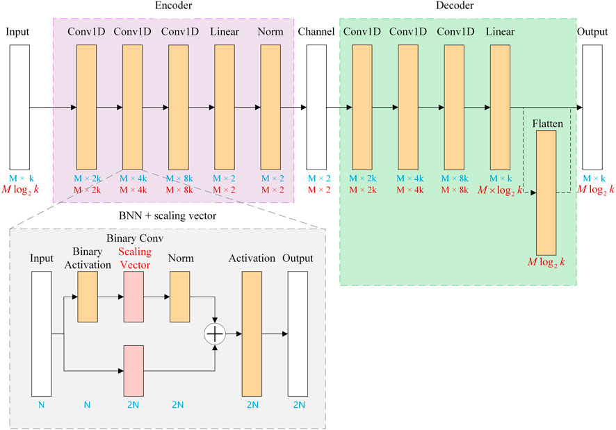
FIGURE 2. Structure for the encoder and decoder.

The input first enters the network through an input terminal and then goes through three successive convolutional layers to achieve the function of parameter training. The three same convolutional layers have different parameters to enhance the training ability of the network. In each convolution layer, there is a normal layer to limit the maximum and minimum values of input vectors to the limit range of the hidden layer and output layer functions. This is followed by a binary linear layer. At this point, the input signal has been perfectly processed into information that can enter the channel. After that, the processed information will first be transformed into the form of constellation map to intuitively reflect the modulation capability of our network. In the channel output end followed by the decoder part, this part of the processing and encoder is just the opposite so as to ensure that the signal channel can be restored to its original form.

The decoder structure is also composed of three convolution layers, in which the parameters are consistent with the encoder. A binary linear layer is also added before the final output. In this way, the whole autoencoder is described completely. It should be noted that the autoencoder model can also be built with dense neural networks, which is achieved by replacing the convolutional layer in our model with the dense layer.

With the autoencoder structure, we binarized the three separate convolutional layers in both the encoder and decoder and kept other structures unchanged. The convolutional layer is replaced by the basic structure diagram marked by the gray box in Figure 2 without the scaling vector shown in red. In this way, the intrinsic autoencoder functionality is not changed, and only the representation of the data is altered, resulting in a significant reduction in computational complexity. First of all, in every single convolutional layer, the data are treated by skip connect. The input of the convolutional layer is separately processed by a single binary convolution and three series of binary operations. The outputs of these two operations will then be combined together to get rid of the effect of residues. The three binary operations are activation, binary convolution, and binary normalization. In the most basic structure for the BNN, the scaling vector in binary convolution is not applied. At last, the combined value is further processed with activation and end up here. The other layers that appear in our autoencoder are in the same form except for layer parameters.

Beyond the existing BNN techniques described earlier, we made three modifications empirically and achieved a better performance. First, we added scaling vector in the binary convolutional layer. It is clearly shown in Figure 2 that the only difference we placed is the addition of the scaling vector compared to our fundamental BNN structure. Likewise, this structure is applied in every convolutional layer in our autoencoder. Second, based on the fundamental BNN structure, we added shifting layers into the network, which is shown in Figure 3. In this modification, the scaling vector is not added at first to ensure a clear comparison between the basic structure and the structure with a single change of shifting. At this stage, the input should be shifted before proceeding with the three series binary layers. There is another shifting that appears at activations. The activation experiences shifting before processing with the prepared binary data. After the activation, the last shifting layer appears and then, the data of this convolution layer are output. The other layers both in the encoder and decoder are adjusted as well, and this is the network structure taking the idea of activation shifting and reshaping. Third, we combined both the method of shifting and addition of the scaling vector as a whole, and results in the structure are depicted in Figure 3. Under this modified structure, the binary convolution is added with the scaling vector, and the three-shifting described in the second modification are also included.

FIGURE 3

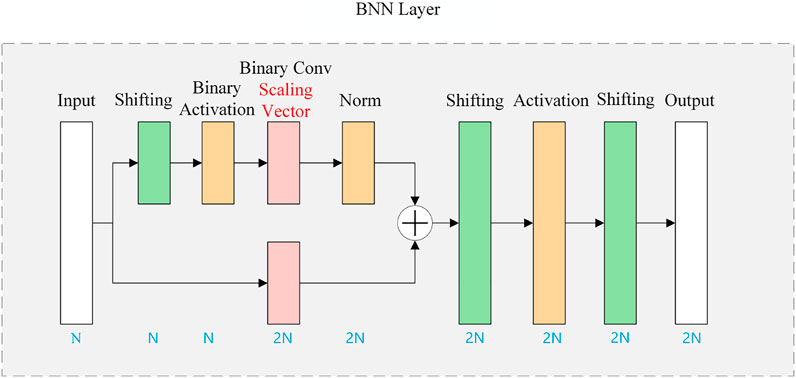
FIGURE 3. Structure for the BNN layer as pure shifting and with the scaling vector.

4 Simulation Results

4.1 Setting

The transmission size M is set to be 400, and the modulation order k is 64. In other words, the system takes 400 symbols as input for every time, where each symbol contains 6-bit information. The kernel size and stride in the convolution layer are both 1. The batch size B is 32 for training with a single run of 30 epochs. Our learning rate is 1 × 10⁻3 and is effectively fixed, and our optimizer uses Adam. The loss function uses binary cross entropy and multi-class cross entropy, which are used for end-to-end training. These parameters are consistent with all the structures ranging from dense, CNN to BNN.

We constructed a data set using the randomly generated original symbol information$X\in {\left\{\mathrm{0,1,2}\dots 63\right\}}^M$. The data set is distributed independently and will represent the encoder’s input with a one-hot code $X_{\mathit{one-hot}}\in {\left\{\mathrm{0,1}\right\}}^{M\times k}$. Each iteration produces a new set of data, which makes our network more stable. The proposed BNN structure is verified in both the symbol and bit information transmission scenarios. Different activation functions are used for the two scenarios, which is elu for the symbol transmission and tanh for the bit transmission.

As for our structure, the parameters of three convolutional layers and the linear layer in the encoder are trainable, while the normalization layer does not encounter a trainable parameter. This is also true for a decoder as well. Moreover, parameters in shifting, binary convolution, and scaling vector are able to be trained in the BNN structure, and the remaining parameters are not.

4.2 Simulation Results Under the AWGN and Rayleigh Channels

At first, we compared three different network structures: dense, CNN, and BNN for the bit and symbol transmission scenarios. Second, based on the results under the different network structures in the BNN, the proposed modification of the BNN structure is conducted. The two different forms of dense, CNN, and BNN, respectively, used full connection layer, convolution, and binary convolution, while their network structure is the same under the same transmission mode. The network structure based on bit and symbol is basically similar, except that the first convolution of the encoder is changed. The convolution kernel size and slide of the former are 2K and K, respectively, while the latter are both one.

The performance comparison for the symbol transmission is shown in Figure 4. It can be found that the performance based on the three different structures is basically the same and better than the standard 64QAM, indicating that the BNN structure with lower parameters and complexity can achieve the same performance as the dense and CNN models when transmitting symbols. The corresponding constellation map at this time is shown in Figure 5. In comparison with the four constellations, we found that dense and CNN constellations were basically the same, which were closer to the regular hexagon, while the BNN was closer to the regular heptagon.

FIGURE 4

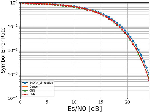
FIGURE 4. Performance comparison when transmitting symbols.

FIGURE 5

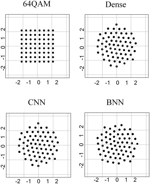
FIGURE 5. Learned constellation maps when transmitting symbols.

Figure 6 shows the performance comparison for the bit transmission. The performance based on the CNN and BNN is similar and better than that under dense. This is because dense has no convolution operation and cannot use the first convolution in the encoder to process the correlation between adjacent information like the CNN and BNN. In addition, the constellation map comparison in the bit scenario is shown in Figure 7, which is consistent with SER’s conclusion that the constellation map of the CNN and BNN is basically the same, while certain constellation points of dense are not aligned, which further leads to its performance degradation.

FIGURE 6

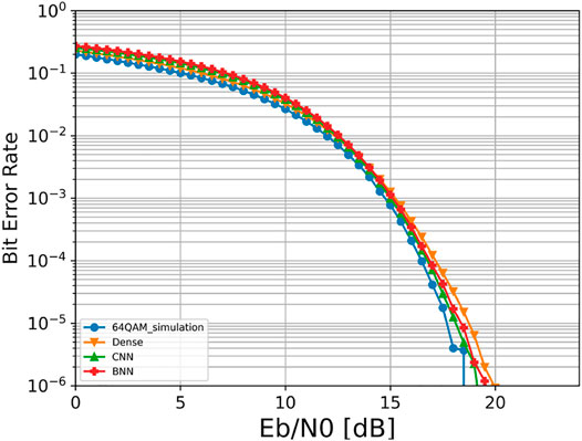
FIGURE 6. Performance comparison under bit.

FIGURE 7

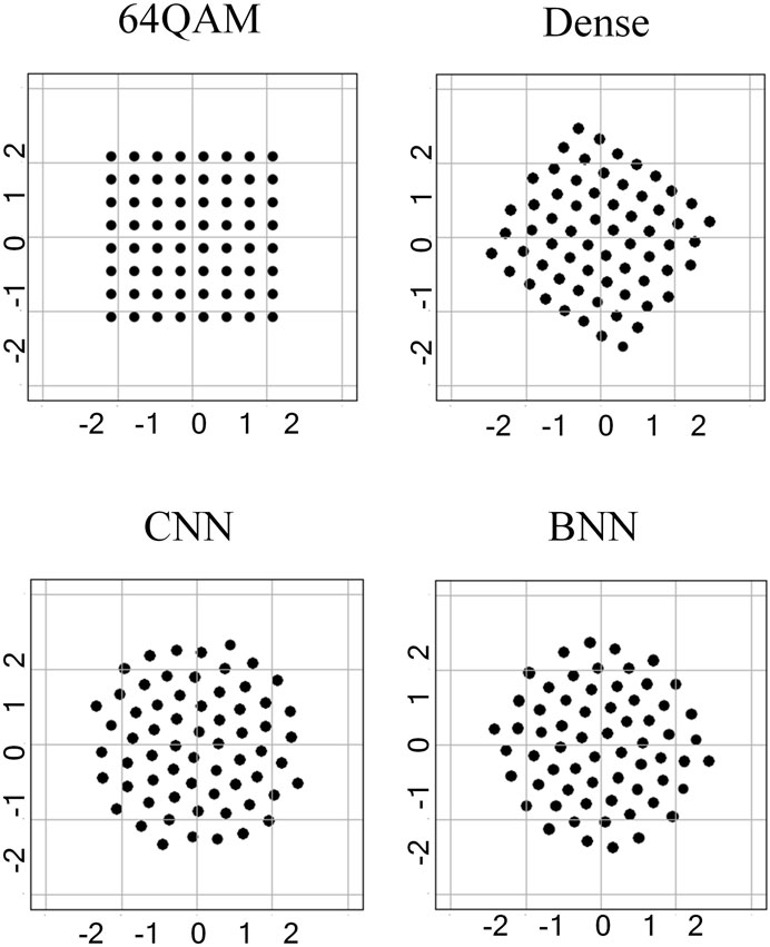
FIGURE 7. Constellation map under bit.

To further test the performance of our network structure in another situation, a Rayleigh channel has been invoked. Figure 8 indicates the performance of four different network structures under the Rayleigh channel. It can be concluded that the structure of the BNN, CNN, and dense show better performance than the standard 64QAM under symbol. The constellation maps of these structures shown in Figure 9 are coherent with the symbol error examination, indicating that our network structure enjoys an excellent generalization ability.

FIGURE 8

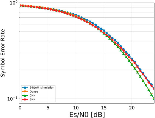
FIGURE 8. The performance of four different network structures under Rayleigh channel.

FIGURE 9

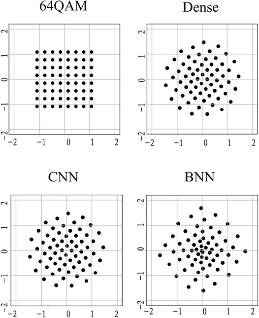
FIGURE 9. Constellation diagrams over Rayleigh under symbol.

The performance of our structures under bit is pretty much the same as standard 64QAM so that renderings are not designed to be shown here for the reasons of space.

4.3 Simulation Results With Different Network Structures in the BNN

Next, we used the same training parameters to conduct experiments for different BNN structures and compared them with the standard 64QAM. All BNN constructs are updated end-to-end based on two-step training. We used ReActNet as the baseline to illustrate the effect of our modification, including removing the scaling vector and shifting part in the BNN structure. In addition, we removed all the changes, leaving only the original BNN structure, and used it to demonstrate the performance change that comes with the binarization of network parameters directly.

The performance comparison of different BNN structures is shown in Figure 10. By observing the image, it is not difficult to find that the symbol error rates of the two network structures without scaling vector are close to 1, showing that the network cannot distinguish any information at all. This indicates that direct binarization of the network results in the loss of information, and removing the scaling vector will have a devastating impact on network performance. It is due to the existence of the scaling vector that the network retains as much information as possible while ensuring binarization and provides favorable conditions for subsequent gradient propagation. Furthermore, we found that the performance of the structure in removing shifting part is slightly better than the standard ReActNet, and this conclusion can also be obtained when the original BNN structure is compared with the ReActNet structure when the scaling vector is removed. The conclusion of this experiment may be related to the different information transmitted through the network. Since BNN transmits 64QAM-based signals rather than the complex images transmitted by ReActNet, the conclusion that the addition of the shifting part to images favors further information retention is no longer tenable.

FIGURE 10

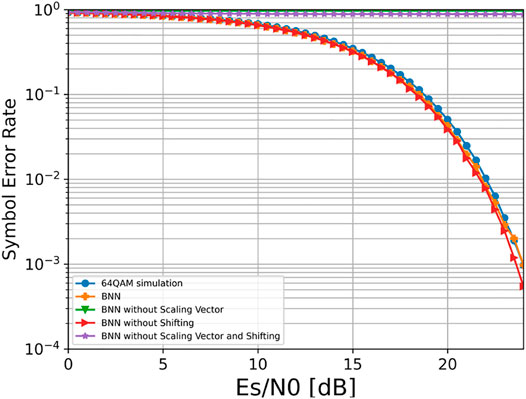
FIGURE 10. Performance comparison of different BNN structures.

A comparison of constellations under different BNN structures is shown in Figure 11. The constellation points learned by the two network structures excluding the scaling vector cluster together, and thus, the constellation diagrams obviously did not show any regularity, which are consistent with their experimental results that SER was close to one. On the other hand, the constellation map of the standard ReActNet and the shifting part removed network are very similar, both approximating a regular polygon, which results in the maximum Euclidean distance between adjacent constellation points and thus exhibiting a good performance.

FIGURE 11

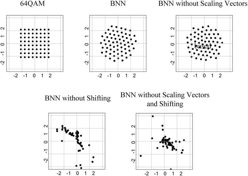
FIGURE 11. Comparison of constellations under different BNN structures based on ReActNet.

4.4 Complexity Analysis

Based on the two different information transmission experiments in symbol and bit, the parameters of three network structures in dense, CNN, and BNN are shown in Table 1. In the case of bit transmission, the parameters of dense are similar to those of the CNN at both the transmitter and the receiver end. With CNN as the baseline, the parameters of the entire system based on BNN are 14.42% of the CNN with the same network structure. In the symbol-based transmission method, the parameters of dense are the same as CNN, which is 4.72 times of the BNN. Considering that binarized data occupy only 1 bit while one float in full precision network takes up 16 bits, it can be concluded that the proposed BNN model saves the storage complexity largely.

TABLE 1

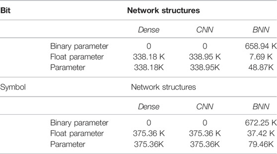
TABLE 1. Parameter size being updated in networks.

The floating-point operations (FLOPs) of different information transmission models are shown in Table 2. In the case of bit, the FLOPs of dense networks are slightly less than those of the CNN, while those of the BNN are only 14.06% with the same structure which has the same result in network parameters. When transmitting the symbol, the FLOPs of dense and CNN are same, which is about five times that of the BNN. It should be noted that the complexity of the bit operation is one-sixteenth of that of the floating-point operation. Hence, the BNN structure can greatly reduce the computation complexity of the data transmission model.

TABLE 2

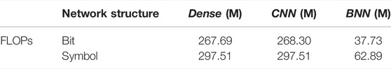
TABLE 2. Computational complexity of networks.

5 Conclusion

In this study, we proposed a BNN-based autoencoder communication network structure and made modifications to further improve its performance. Experimental results showed that the modulation and demodulation system based on the BNN proposed in this study can achieve the same effect as the CNN while effectively reducing the complexity, in both the bit and symbol transmission scenarios. In addition, the scaling vector is necessary for network binarization, and removing the shifting part is beneficial for the data transmission. Furthermore, the proposed BNN structure can be integrated into the existing neural communication models beyond modulation and demodulation and can achieve better performance than model-based techniques.

Data Availability Statement

The original contributions presented in the study are included in the article/Supplementary Material; further inquiries can be directed to the corresponding author.

Author Contributions

CB and LX completed the experiments, CZ provided guidance and research direction, and HQ proposed ideas and directed experiments. All the authors completed the manuscript writing together.

Funding

This work was supported in part by the National Key R&D Program of China under Grant 2020YFB1805703, and in part by the National Natural Science Foundation of China under Grant 62101102.

Conflict of Interest

The authors declare that the research was conducted in the absence of any commercial or financial relationships that could be construed as a potential conflict of interest.

Publisher’s Note

All claims expressed in this article are solely those of the authors and do not necessarily represent those of their affiliated organizations, or those of the publisher, the editors, and the reviewers. Any product that may be evaluated in this article, or claim that may be made by its manufacturer, is not guaranteed or endorsed by the publisher.

References

Cammerer, S., Aoudia, F. A., Dörner, S., Stark, M., Hoydis, J., and ten Brink, S. (2020). Trainable Communication Systems: Concepts and Prototype. IEEE Trans. Commun. 68 (9), 5489–5503. doi:10.1109/tcomm.2020.3002915

CrossRef Full Text | Google Scholar

Chen, Y.-H., Krishna, T., Emer, J. S., and Sze, V. (2017). Eyeriss: An Energy-Efficient Reconfigurable Accelerator for Deep Convolutional Neural Networks. IEEE J. Solid-State Circuits 52 (1), 127–138. doi:10.1109/jssc.2016.2616357

CrossRef Full Text | Google Scholar

Felix, A., Cammerer, S., Dörner, S., Hoydis, J., and Ten Brink, S. (2018). “Ofdm-autoencoder for End-To-End Learning of Communications Systems,” in 2018 IEEE 19th International Workshop on Signal Processing Advances in Wireless Communications (SPAWC), 1–5. doi:10.1109/spawc.2018.8445920

CrossRef Full Text | Google Scholar

Han, S., Mao, H., and Dally, W. J. (2015). Deep Compression: Compressing Deep Neural Networks with Pruning, Trained Quantization and Huffman Coding. arXiv preprint arXiv:1510.00149.

Google Scholar

Hinton, G. E., and Salakhutdinov, R. R. (2006). Reducing the Dimensionality of Data with Neural Networks. Science 313 (5786), 504–507. doi:10.1126/science.1127647

PubMed Abstract | CrossRef Full Text | Google Scholar

Jiang, Y., Kim, H., Asnani, H., Kannan, S., Oh, S., and Viswanath, P. (2019). Turbo Autoencoder: Deep Learning Based Channel Codes for Point-to-point Communication Channels. Adv. Neural Inf. Process. Syst. 32.

Google Scholar

Kung, J., Zhang, D., van der Wal, G., Chai, S., and Mukhopadhyay, S. (2018). Efficient Object Detection Using Embedded Binarized Neural Networks. J. Sign Process Syst. 90 (6), 877–890. doi:10.1007/s11265-017-1255-5

CrossRef Full Text | Google Scholar

Liu, Z., Shen, Z., Savvides, M., and Cheng, K.-T. (2020). Reactnet: Towards Precise Binary Neural Network with Generalized Activation Functions. Euro. Conf. Comput. Vision, 143–159.

CrossRef Full Text | Google Scholar

Liu, Z., Wu, B., Luo, W., Yang, X., Liu, W., and Cheng, K.-T. (2018). “Bi-Real Net: Enhancing the Performance of 1-bit Cnns with Improved Representational Capability and Advanced Training Algorithm,” in Proceedings of the European Conference on Computer Vision (ECCV), 722–737.

CrossRef Full Text | Google Scholar

O’Shea, T., and Hoydis, J. (2017). An Introduction to Deep Learning for the Physical Layer. IEEE Trans. Cognitive Commun. Netw. 3 (4), 563–575. doi:10.1109/TCCN.2017.2758370

CrossRef Full Text | Google Scholar

Qin, H., Gong, R., Liu, X., Bai, X., Song, J., and Sebe, N. (2020). Binary Neural Networks: A Survey. Pattern Recognit. 105, 107281. doi:10.1016/j.patcog.2020.107281

CrossRef Full Text | Google Scholar

Samuel, N., Diskin, T., and Wiesel, A. (2017). “Deep Mimo Detection,” in 2017 IEEE 18th International Workshop on Signal Processing Advances in Wireless Communications (SPAWC), 1–5.

CrossRef Full Text | Google Scholar

Stark, M., Ait Aoudia, F., and Hoydis, J. (2019). “Joint Learning of Geometric and Probabilistic Constellation Shaping,” in 2019 IEEE Globecom Workshops (GC Wkshps), 1–6.

CrossRef Full Text | Google Scholar

Vanhoucke, V., Senior, A., and Mao, M. Z. (2011). “Improving the Speed of Neural Networks on Cpus,” in Deep Learning and Unsupervised Feature Learning Workshop (NIPS).

Google Scholar

Wu, N., Wang, X., Lin, B., and Zhang, K. (2019). A Cnn-Based End-To-End Learning Framework Toward Intelligent Communication Systems. IEEE Access 7, 110197–110204. doi:10.1109/access.2019.2926843

CrossRef Full Text | Google Scholar

Ye, H., Ye Li, G., and Juang, B.-H. F. (2020). “Bilinear Convolutional Auto-Encoder Based Pilot-free End-To-End Communication Systems,” in ICC 2020 - 2020 IEEE International Conference on Communications (ICC), 1–6.

CrossRef Full Text | Google Scholar

Zhu, B., Wang, J., He, L., and Song, J. (2019). Joint Transceiver Optimization for Wireless Communication Phy Using Neural Network. IEEE J. Sel. Areas Commun. 37 (6), 1364–1373. doi:10.1109/jsac.2019.2904361

CrossRef Full Text | Google Scholar