Intensified greenhouse gas prediction: Configuring Gate with Fine-Tuning Shifts with Bi-LSTM and GRU System

Introduction: On a global scale, climate change refers to persistent alterations in weather conditions and temperature patterns. These modifications have far-reaching implications across the world. GHGs (Greenhouse Gases) play a crucial role in driving climate change. Most of these emissions originate from human activities, particularly those contributing to releasing CO₂ and CH₄. In the conventional approach, identifying emissions involves recognizing and quantifying the sources and amounts of GHG released into the atmosphere. However, this manual identification method has limitations, including being time-consuming, relying on incomplete resources, prone to human error, and lacking scalability and coverage.

Methodology: To address these challenges, a technology-based system is necessary for effectively identifying GHG emissions. The proposed method utilized the configuration of a gating mechanism incorporating fine-tuning shifts in the Bi-LSTM-GRU algorithm to predict GHG emissions in top-emitting countries. The PRIMAP-host dataset is used in the respective method comprising subsector data such as CO₂, CH₄, and N₂O to attain this. In the presented model, Bi-LSTM is used to capture significant features, handle vanishing gradient problems, etc., because of its process in both directions. Conversely, it is limited by overfitting and long-term dependencies.

Results and discussion: GRU is used with Bi-LSTM to address the issue for the advantages of memory efficiency, handling long-term dependencies, rapid training process and minimizes the overfitting by infusion of GRU in the input layer of BiLSTM with tuning process in the BiLSTM. Here, the configuration of gates with fine-tuning shifts to improve the prediction performance. Moreover, the efficiency of the proposed method is calculated with performance metrics. Where RMSE value is 0.0288, MAPE is 0.0007, and the R-Square value is 0.99. In addition, internal and external comparisons are carried out to reveal the greater performance of the respective research.

1 Introduction

Globally, climate change (Orazalin et al., 2024; Marquet et al., 2024) is a significant problem responsible for various consequences such as temperature rise, challenging weather events, impacts on health, etc. (Tol, 2024; Casey, 2024). Predominantly, GHG emission is the main factor responsible for climate change, where the emission of CO₂ (Ritchie and Roser, 2024), CH₄ (Hu et al., 2024), and N₂O is caused by human activities (Wang and Azam, 2024; Yang et al., 2024; Aljughaiman et al., 2024). It is significant to identify the highly GHG emitted area to concentrate on the significant area to reduce GHG emission (Abdul Latif et al., 2021; Erdoğan et al., 2024). Conventionally, manual identification of GHG emissions includes quantifying and identifying the sources and amount of the GHG emissions in the environment. It is time consuming as it takes days to complete the identifying process. Besides, it requires expert support, which can be expensive regarding resources. Moreover, it can be prone to human error and less efficient. To tackle the issue, conventional researchers utilized AI (Artificial Intelligence) for the advantages of automation, pattern recognition, scalability, and adaptability. It delivers several advances with greater efficiency in the prediction mechanism with the ML (Machine Learning) and DL algorithms.

Correspondingly, enormous traditional systems utilized various techniques to attain better efficiency for GHG emissions. For instance, three categories of regression systems have been used in the existing method to predict soil GHG emissions (Adjuik and Davis, 2022). Here, CO₂ and N₂O with diverse environmental agronomic and soil data have been extracted for five years in Canada (Pelster et al., 2021). Besides, statistical analysis has been performed, and cross-validation has been performed to evaluate the efficacy of the classical system. The experimental results signify that the existing model accomplished an RMSE value of 0.87, which indicates better efficiency than the conventional system (Hamrani et al., 2020). Accordingly, GHG emission forecasting has been processed in terms of electricity production in traditional research. To attain this, SVM (Support Vector Machine) and ANN (Artificial Neural Network) have been utilized to predict factors such as N₂O, CH₄, and CO₂. Moreover, 2015 to 2018 has been collected for the prediction mechanism. The outcome of the experiment signifies better performance (Bakay and Ağbulut, 2021). Correspondingly, hybrid mechanisms have been constructed for forecasting GHG emissions. To accomplish this, energy market data has been used in the traditional system. Here, five indices are used, and nine ML-based algorithms are compared. Lastly, stepwise regression techniques are used to determine the similarity among the data. Better efficiency has been identified through the prediction results of the conventional model (Javanmard and Ghaderi, 2022). Likewise, enormous existing research is utilized to predict GHG emissions but is limited through efficiency, speed, and overfitting of data.

To address the problem, the projected method used Configuring Gate with Fine-Tuning Shifts with Bi-LSTM and GRU System. Initially, PRIMAP-his dataset is loaded in the system where a pre-processing technique is utilized for formulating the dataset for the prediction with data cleaning and standardized scales method. Further, data splitting is used to evaluate and train the projected system with the ratio of 80:20. At this time, Configuring Gate with Fine-Tuning Shifts with Bi-LSTM and GRU System is used for the prediction of GHG emission in the top emitting countries such as China, European Union, Indonesia, Russia and the United States. Finally, the performance of the respective model is calculated using the performance metrics. Moreover, comparative analysis is carried out to evaluate the efficacy of the proposed method. Correspondingly, the major contribution of the proposed model is signified in the following:

To employ Configuring Gate with Fine-Tuning Shifts with Bi-LSTM and GRU System with PRIMAP-his dataset for enhancing the prediction of GHG emission in the top emitting countries. To apply performance metrics to calculate the efficiency of the projected system. To function internal and external comparison to evaluate the proposed prediction efficiency.

The paper is organized based on the productive approaches applied in forecasting GHG emissions by examining prevailing researchers discussed in Section 1. Whereas Section 3 indicates the method of the proposed system. Further, the results attained by the presented model are illustrated in Section 4. Finally, the conclusion with the future work of the projected mechanism is signified in Section 5.

2 Review of literature

The section analyzes conventional research on the prediction of GHG emissions.

The gas field production has been forecasted in the traditional model. Here, the CNN-LSTM system has been used to predict. Even though the approached study still does not emphasized the prospective overfitting problems combined with DL models (Li et al., 2022; Han et al., 2023; He et al., 2020). Besides, the dataset has been acquired from the monthly natural gas prediction data from southwest China. The result of the prediction illustrates better efficiency. However, the approached model has not been able to integrate variables such as seasonal changes and economic activity (Zha et al., 2022). Similarly, comparative analysis has been performed in the classical system to forecast CO₂ emissions. Still the approached study has not been capable to seizure due to the limitations of particular timing of measurements and number of sampling (Ajwang'Ondiek et al., 2021; Ding et al., 2023; Wen and Cao, 2020). For the analysis, a multivariate polynomial regression system and DL-based technique have been used for comparison. In addition, it analyzes the similarity among the electrical energy consumption, CO₂, and GDP for the Bangladesh region. Though the approached study has only focused on the mission from Bangladesh region and it does not focused on other regions (Hasan and Chongbo, 2020). The prediction outcome depicts the better efficacy of the classical prediction. Nevertheless, the existing study only focused on the emissions of CO₂ and does not deliberate other GHG which contributed to climatic change (Faruque et al., 2022). Likewise, LSTM-based architecture (Gong et al., 2021; Esparza-Gómez et al., 2023) has been constructed to predict greenhouse climate. The limitation of the prevailing study deliberated on identifying the greenhouse crop yields by DL algorithms that restricted their significance to wider the strategies of climate change mitigation. Here, climate data has been used for greenhouse prediction. The experimental results illustrate the better efficiency of conventional research. The interpretability of the LSTM model is more complex that may delay the real-time applications in greenhouse management (Liu et al., 2022). A hybrid prediction framework for air quality has been integrated with XGBoost and W-BiLSTM (PSO)-GRU techniques. In order to predict soil greenhouse gas (GHG) emissions. Due to the incomplete and inconsistent data can led to untrustworthy prediction (Al-Nefaie and Aldhyani, 2023; Biswas et al., 2021a) from an agricultural field, deep learning and ML regression models were investigated. The results showed that R2 values of PM2.5, PM10, SO₂, CO, NO₂ and O₃ predictions exceeded 0.94, and MAE and RMSE values were lower than 0.02 and 0.03. Because of the integration of the BiLSTM, XGBoost and GRU caused complexity which has complicated the interpretation and training of the model. It was challenging to predict the involvement of individual predictions (Chang et al., 2023).

LSTM model outperformed other considered machine learning (ML) models, with the highest R coefficient and lowest root mean squared error (RMSE) values, according to thorough analysis that included statistical comparison and cross-validation for the prediction of CO₂ and N₂O fluxes. The prevailing study has used concentration weighted trajectory analysis and bivariate polar plots which have intrinsic limitations in precisely seizing the sources of gas emissions and their dynamics (Kim et al., 2020). The prediction accuracy of the proposed BiLSTM model has been compared with two existing models, namely Auto-Regressive Integrated Average Moving (ARIMA) and Chaos Time Series (CHAOS). According to experiment results, the t-SNE_VAE_bi-LSTM model forecasted mean square error (MSE) has been less accurate than ARIMA and CHAOS models, with MSE values of 0.029 and 0.069 for CH₄. The study has employed ML approaches that have challenges in seizing complicated relationships and interfaces among variables which have been affected by methane emissions (Venkateshalu and Deshpande, 2023; Patole, 2021; Jongaramrungruang et al., 2022; Yuan et al., 2022), 0.037 and 0.019 for CO₂, 0.092 and 0.92 for CO (Kumari and Singh, 2023; Namboori, 2020), 1.881 and 1.892 for O₂, and 1.235 and 1.200 for H₂. A Bi-LSTM-based CO₂ emission prediction model has been developed. The existing study has struggled with the quality and availability of the data that has impacted the prediction accuracy (Widi Hastomo et al., 2022). The Bi-LSTM model performed better, as evidenced by lower MAE, MSE, and MAPE values than the LSTM and GRU approaches. The study has employed BiLSTM which was difficult and complicated that can delay considerate of the features contributed for the patterns of carbon emission (Aamir et al., 2022). In terms of accuracy, the BiLSTM model outperformed the others, achieving high MSE and RMSE prediction values. The highest possible (R² = 93.78) has been achieved by the BiLSTM model. Furthermore, R percent has been deployed to identify a relationship between the dataset’s attributes to determine which attributes had the strongest correlation with CO₂ emissions. The prevailing study has faced model limitation that the ML algorithms cannot be ideal for all types of noxious waste and effectively led to biased estimates (Hien and Kor, 2022; Biswas et al., 2021b).

Likewise, Regression coefficients of 0.87, 0.62, 0.84, 0.67, 0.75, and 0.72 were obtained to predict the concentrations of pollutants O₃, PM2.5, PM10, NO₂, and SO₂. The outcomes demonstrated that hourly air pollutant concentrations can be reliably predicted using the Bi-LSTM deep neural network model. Using these data(s), which carried 90, 95, and 100% of the original dataset’s information for 100 epochs, GRU, LSTM, and Bi-LSTM techniques were applied. Out of the three deep learning methods, we found that the GRU worked the best. As stated in reference, the corresponding values of RMSE and CS were (0.0777, 0.9735), (0.0837, 0.9728), and (0.0780, 0.9740). The Bi-LSTM model showed a mean square error of 52 points 99 percent, a relative mean square error of 7 points 28 percent, a mean absolute error of 3 points 4 percent, and an R-square of 97 percent. The approached study has not displayed all features which are triggering air quality such as local industrial activities, meteorological conditions and seasonal variations. These features can majorly impact the quality of air but these have not fully seizure by the study (Taylor and Ezekiel, 2023). The model was evaluated using several parameters, including mean square error, absolute error, absolute mean square, and R2 square for the gases carbon monoxide and carbon dioxide dot. The best bio-signal performance is achieved by BiLSTM with Bahdanu Attention. One of the datasets yields the best results for LSTM, with an MAE of 0.70 ± 0.02. The two datasets with the highest results were obtained using Bi-LSTM with Bahdanau attention; the MAE for sEMG-based data was 0.51 ± 0.03, while for PPG and ECG-based data, it was 0.24 ± 0.03. The lack of transparency delay the cli9nical acceptance and the capability to comprehend the essential features triggering the predictions (Kumar et al., 2022).

2.1 Problem identification

• The existing study majorly intensive on CNN-LSTM model for predict the carbon emission still does not emphasis the prospective overfitting problems combined with DL models. The lackness in comprehensive dataset which contains different prompting features might also restrict the generalizability and accuracy of the model (Li et al., 2022).

• The prevailing research incorporate CNN and LSTM for precise predictions over 30 Chinese fields. The study cannot describe the regional variance in data availability and carbon emission features. The performance of the model is limited by the granularity and quality of the input data during training (Han et al., 2023).

• The limitations of the existing research is the predictive capacity of the model and it does not integrate variables such as seasonal changes and economic activity (Zha et al., 2022).

3 Proposed methodology

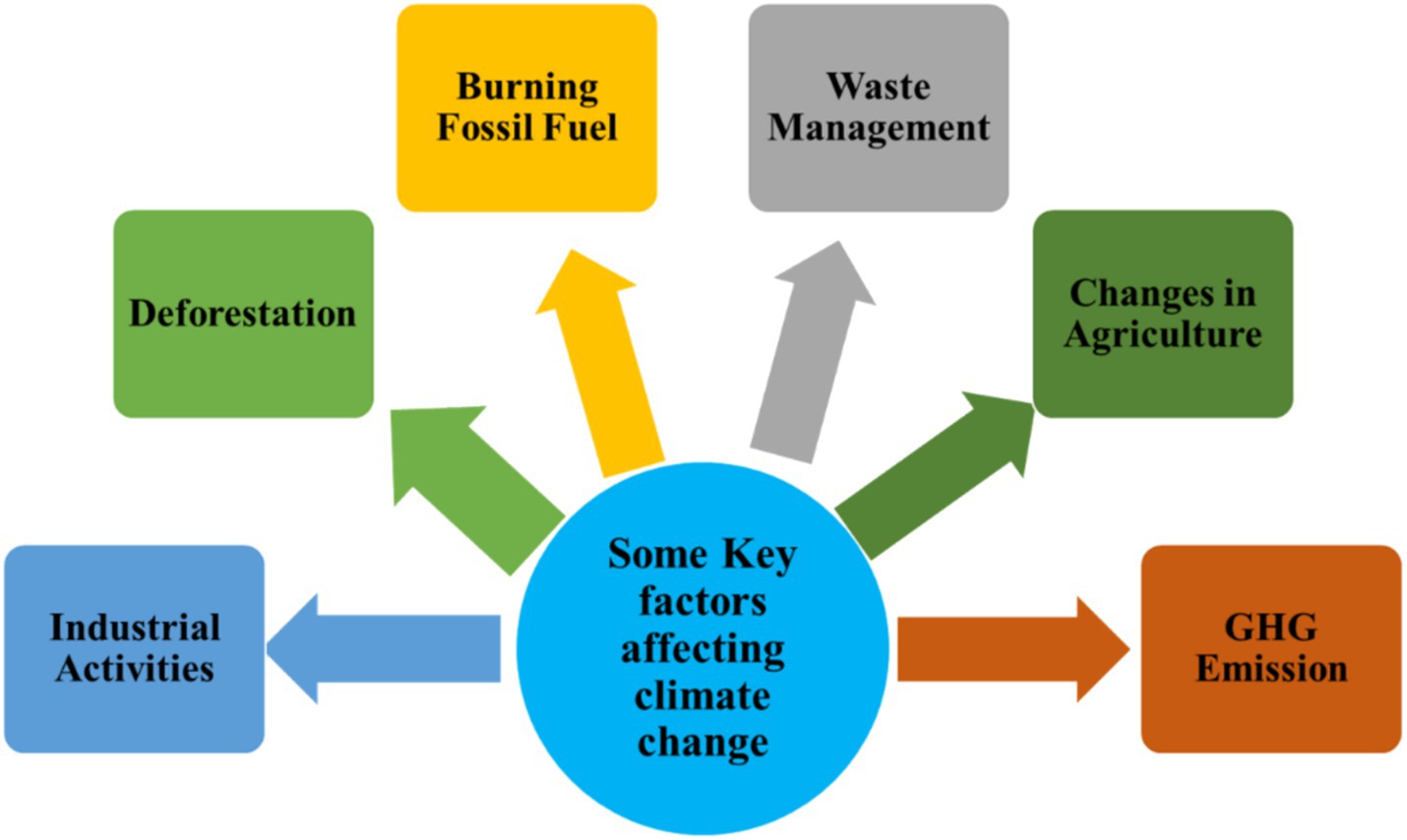
Globally, climate change is the continuing change in the weather and temperature patterns which leads to several consequences worldwide. Rising temperatures, life-threatening weather actions, ecosystem disruption, coral bleaching, ocean acidification, and impacts on human health are significant concerns caused by climate change. The emission of GHG (Greenhouse Gas) that cause climate change which maximized to 50 fold since from the mid-1800s. Followed by agriculture, the energy creates almost three-quarters of global emissions. Followed by manufacturing and transportation, splitting down the energy field into its sun-sectors, heat and electricity generation produces the major portion of emission. These consequences of climate change are extensive and create essential challenges for the world. Accordingly, climate change is a complex phenomenon that is disturbed by various factors. Figure 1 represents the substantial factors affecting the climate change.

Figure 1

Figure 1. Factors affecting climate change.

It signifies the reasons that are responsible for climate change. Several factors influence climate change, such as greenhouse gas emissions, deforestation, changes in the usage of the land, industrial activities, waste management, population, etc. Significantly, GHG is the chief driver of climate change, where most of the disturbing emission is produced due to the activities of humans, such as CO₂ and CH₄. Besides, clearing of trees enhances atmospheric absorption of GHGs. Moreover, population and industrial functions like energy production and manufacturing mining release essential amounts of GHS into the atmosphere. Accordingly, the burning of fossil fuels, industrial functions, and several other factors contribute to the GHG emissions of the world. Here, greenhouse gas emission is the chief driver of climate change. Correspondingly, Figure 2 denotes the negative consequences of GHS in the world.

Figure 2

Figure 2. Negative consequences of greenhouse gas.

Negative consequences of GHG emissions are present in the world. It has turned out to be a global concern where N₂O, CH₄, and CO₂ contribute to the deceiving heat in the atmosphere. The major consequences of GHG are climate change, rising sea levels, loss of biodiversity, health effects, economic concerns, etc. Accordingly, GHG has detrimental effects on the world. The coordination of industries, governments, and individuals on the earth is needed to work together to minimize GHG. Besides, implementing climate policies and sustainable practices is essential to achieve a GHG emission-free world. Correspondingly, the identification of GHG emission scores is needed to implement particular policies and practices to reduce GHG emissions. It assists in identifying chief contributions to emissions and enabling the government to prioritize mitigation efforts and assign resources. Overall, it aids in developing tailored solutions for minimizing GHG emissions and fighting climate change worldwide.

Traditionally, manual identification of GHG emissions includes recognizing and enumerating the sources and value of GHG released into the atmosphere. Accordingly, manual identification involves several limitations such as time-consuming, incomplete resources, human error, lack of scalability and coverage, etc. To resolve the issue, a technology-based system is needed to effectively identify GHG emissions. To attain this, enormous traditional research utilized DL-based technology to achieve advantages such as automation, pattern recognition, adaptability, and scalability. However, it lacks a few factors like accuracy, speed, and handling larger datasets.

Significantly, to address the problem, the proposed system utilized a specific set of techniques to classify GHG emissions. Figure 3 signifies the methodological design of the presented model.

Figure 3

Figure 3. Methodological flow of respective research.

It is identified that the proposed mechanism comprises data collection, pre-processing, data splitting, and classification. The subsequent sections represent the precise explanation of the respective approach.

3.1 Data collection

The proposed method used the PRIMAP-host dataset for the classification of GHG emissions. The publicly available database syndicates enormous published datasets to deliver a complete set of GHG emission pathways for every country. Besides, it revolves around the main IPCC (Intergovernmental Panel on Climate Change) 2006 types. The span of dataset from the year of 1850 to 2018, offering a historical aspects on GHG emission across 168 years. The dataset contains emission from a major number of countries along with the report emphasizing, which 64% of worldwide GHG emissions are indorsed in just 10 countries. The dataset seizures emissions from both low-emitting and high-emitting nations. The dataset gathers the data of emissions from various sources such as GCP, CAIT, UNFCCC and PIK that cooperatively cover a broad array of sectors and countries. It categorized the emissions by six essential economic fields such as waste management, agriculture, industrial processes, bunker fuels and land-use forestry or change. Moreover, it comprises subsector data such as CO₂, CH₄, and N₂O for agriculture, industrial function, and energy.

3.2 Pre-processing

The pre-processing mechanism is used to prepare the dataset for the classification. Here, the data cleaning and standardized scales model is utilized in the proposed system. Accordingly, data cleaning is setting or eliminating incorrect or duplicate data in the dataset. In the respective method, duplicate and missing values are identified to ensure the quality and reliability of data. Besides, a standard scalar eliminates scaling and mean-to-unit variance.

3.3 Data splitting

Data splitting is the method used to test and evaluate the proposed method. For that purpose, data in the respective research is divided into 80:20, where 80 portions are used for training, and 20 portions are used for testing.

3.4 Classification

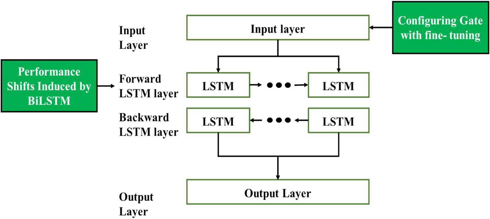
The presented system utilized the configuration of a gating mechanism incorporating fine-tuning shifts in the Bi-LSTM-GRU algorithm. It optimizes the behavior of the gate by refining the shift parameters in the system, which improves the accuracy and adaptability of the network. In the systematic experimentation, the efficacy of the configuration is validated, and improved efficiency aids the sequential data. Figure 4 signifies the architecture of the respective system.

Figure 4

Figure 4. Architecture of the presented model.

It is identified that the proposed model utilized the advantages of LSTM and GRU to predict GHG emission data. The precise explanation of the respective model is signified in section 3.4.1.

3.4.1 Configuring Gate with Fine-Tuning Shifts with Bi-LSTM and GRU

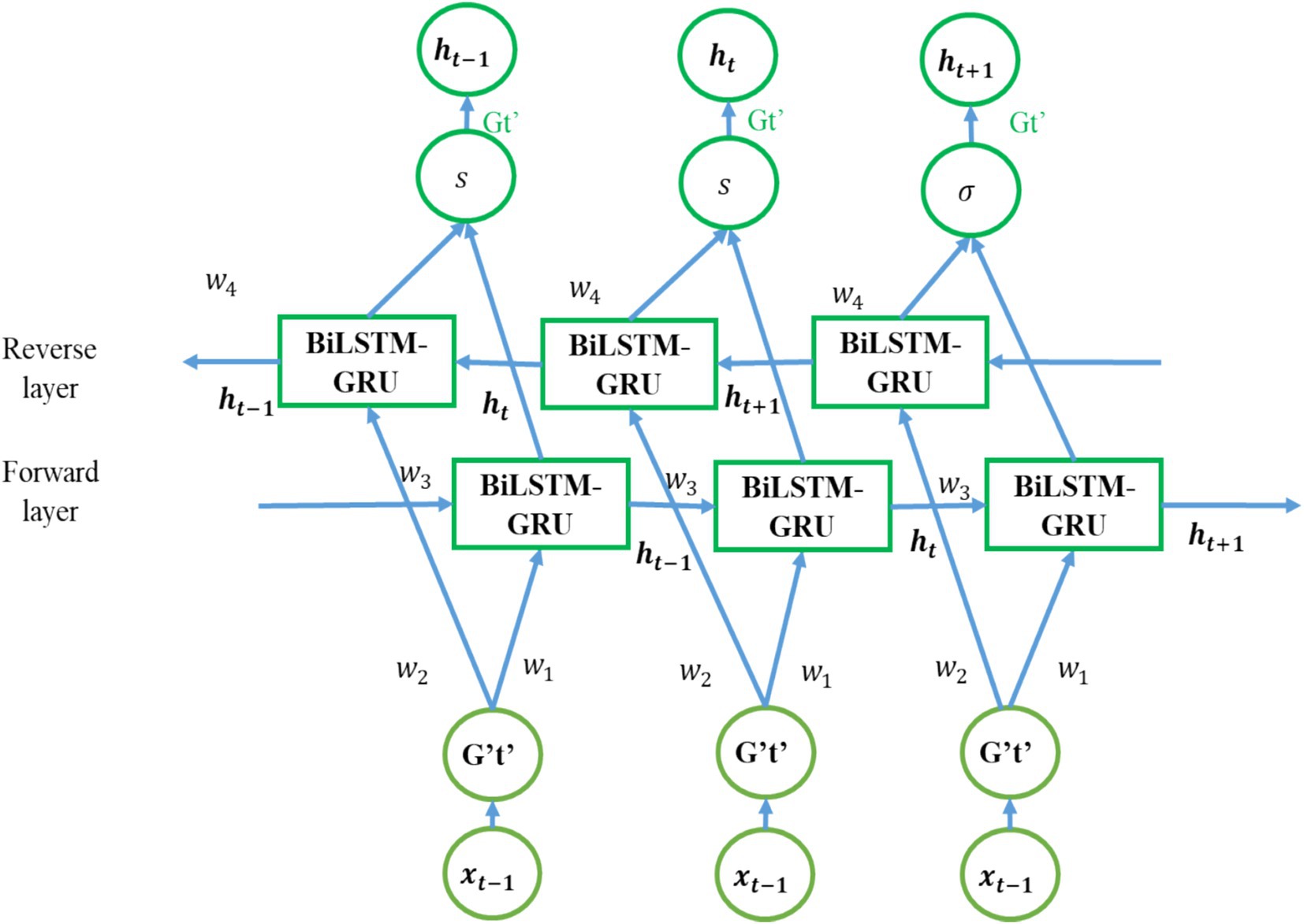
The proposed system configures Gate with fine-tuning Shifts with Bi-LSTM, and GRU is used to predict GHG emission data. In the presented system, Bi-LSTM is used to capture significant features, handle vanishing gradient problems, etc. However, it is lacking long-term dependencies and overfitting. To resolve the issue and to enhance the efficiency, GRU is used with Bi-LSTM for the advantages of memory efficiency, and handling long-term dependencies by infusion of GRU in the input layer of BiLSTM with tuning process in the BiLSTM. Besides, the configuration of gates with fine-tuning shifts to improve the prediction performance. Figure 5 represents the mechanism of configuring the Gate with fine-tuning Shifts with Bi-LSTM and GRU.

Figure 5

Figure 5. Configuring Gate with Fine-Tuning Shifts with Bi-LSTM and GRU.

The proposed Bi-LSTM process the data in both backward and forward directions that can be advantageous if earlier and future background is significant for predictions. The BiLSTM improves the conventional LSTM by processing the data in both forward and backward directions and permitting it to seizure perspective from the emissions of past and future simultaneously. Especially, it is useful for accepting the current emission based on the influence of historical trends. On the other side, the GRU simply the LSTM structure while maintaining its capability to handle long-range dependences and generating them with effective computation. The gating mechanism of proposed GRU aid in forgetting or remembering information that is significant for modeling the complicated relationship among different emission resources and their sequential changes. Hence, it led to enhanced generalization because, the fine tuning aids the proposed model to adjust better to the particular features of the dataset. Altering the learning rates will aid convergence of proposed model more efficiently and restricting overshooting the optimal solution. The performance of the proposed model is improve by the fine tune technique. Here, the optimization of gate behavior is refined by the shift parameters, which improves the precision and adaptability of the information flow in the network. Accordingly, the effectiveness of the configuration is evaluated with systematic experimentation, which will improve the efficiency of sequential data processing. Correspondingly, it is intended to refine the mechanism of gates function in the respective model.

The significant layers of the respective model comprise an embedding layer, bidirectional layer, attention layer, and output layer. In the embedding layer, consider the n values, which are signified in the Equation 1.

$\begin{array}{ll}{m}_{y+1},\dots .m_1,m_{2,}{m}_3& (1)\end{array}$

In the Equation 1 represents the input series of the respective method. In the system, the concatenation of right and left outcome functions with element-wise addition is illustrated in Equation 2.

$\begin{array}{ll}\overleftrightarrow{q}=\overrightarrow{q}\oplus q⃐& (2)\end{array}$

Here, the last review matrix is forwarded to the classification layer in the system. Further, calculations in the first hidden layer and subsequent hidden layer. Equations 3–8 illustrate the first hidden layer in the system.

$\begin{array}{ll}{i}_t=\partial \left(z_i\left[q_{t-1},m_t\right]+b_i\right)& (3)\end{array}$

$\begin{array}{ll}{k}_t=\partial \left(z_f\left[q_{t-1},m_t\right]+b_k\right)& (4)\end{array}$

$\begin{array}{ll}{o}_t=\partial \left(z_o\left[q_{t-1},m_t\right]+b_o\right)& (5)\end{array}$

$\begin{array}{ll}p~t=\tau \left(z_p\left[q_{t-1},m_t\right]+b_c\right)& (6)\end{array}$

$\begin{array}{ll}{p}_t={k_t}^{°}{p}_{t-1}+{i_t}^{°}p~t& (7)\end{array}$

$\begin{array}{ll}\overrightarrow{h_t}={o_t}^{°}\tau \left(p_t\right)& (8)\end{array}$

Correspondingly, Equations 9–14 signifies the second hidden layer in the system.

$\begin{array}{ll}{i}_t=\partial \left(z_i\left[q_{t+1},m_t\right]+b_i\right)& (9)\end{array}$

$\begin{array}{ll}{k}_t=\partial \left(z_f\left[q_{t+1},m_t\right]+b_k\right)& (10)\end{array}$

$\begin{array}{ll}{o}_t=\partial \left(z_o\left[q_{t+1},m_t\right]+b_o\right)& (11)\end{array}$

$\begin{array}{ll}p~t=\tau \left(z_p\left[q_{t+1},m_t\right]+b_p\right)& (12)\end{array}$

$\begin{array}{ll}{p}_t={k_t}^{°}{p}_{t+1}+{i_t}^{°}p~t& (13)\end{array}$

$\begin{array}{ll}\overrightarrow{h}={o_t}^{°}\tau \left(p_t\right)& (14)\end{array}$

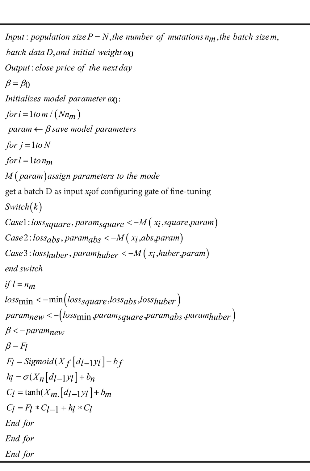
Here, $i_t$ , $k_t$ , and $o_t$ signify three diverse factors: input, forget, and output gate. Accordingly, $W_i$ , $W_f$ , $W_o$ , and $W_c$ depict the weight matrix of the input gate where $°$ illustrates the Hamdard product and $\tau$ signifies the tangent function. Moreover, $h_{t-1}$ and $h_{t+1}$ demonstrates future hidden states. Correspondingly, $b_i$ , $b_k$ , $b_o$ , and $b_c$ . The Algorithm 1 represent the Configuring Gate with Fine-Tuning Shifts with Bi-LSTM and GRU mechanisms.

Algorithm 1 Configuring Gate with Fine-Tuning Shifts with Bi-LSTM and GRU

3.4.2 Long short-term memory

The LSTM is the kind of RNN (Recurrent Neural Network) which is the widely used DL model. It is constructed to solve the vanishing gradient problem. The advantages of LSTM are capturing long-term dependencies, handling vanishing gradients, and flexibility in sequence lengths. Consistently, LSTM layers are cell state, input gate, forget gate, output gate, and hidden state. All the components function as sequential data, which permits capturing long-term dependencies and recollecting significant data. Several LSTM layers are composed to do complex methods like classification and prediction. Correspondingly, the gate of LSTM is represented in Equation 15.

$\begin{array}{ll}{i}_t=\sigma \left(W_i\left[h_{t-1},m_t\right]+b_i\right)& (15)\end{array}$

In the Equation 1, 0 or 1 is the value of $h_{t-1}$ and $m_t$ . Further, if the output is zero, the current will be stocked. The calculation function comprises two parts which are represented in the Equation 16 and 17.

$\begin{array}{ll}{k}_t=\sigma \left(W_f\left[h_{t-1},m_t\right]+b_k\right)& (16)\end{array}$

$\begin{array}{ll}\widetilde{c_t}=tanh\left(W_c\left[h_{t-1},m_t\right]+b_c\right)& (17)\end{array}$

Accordingly, one part is to define the significant data to add to the unit status through the signed activation function. Besides, the other part is to utilize the tanh activation function to form the new vector to upgrade the unit status.

$\begin{array}{ll}{c}_t=k_t\ast c_{t-1}+{i_t}^{°}\widetilde{c_t}& (18)\end{array}$

$\begin{array}{ll}{o}_t=\sigma \left(W_o\left[h_{t-1},m_t\right]+b_o\right)& (19)\end{array}$

$\begin{array}{ll}\overrightarrow{h_t}=o_t\ast tanh\left(c_t\right)& (20)\end{array}$

However, it has certain drawbacks that limit the efficiency of the classification, such as computational complexity and overfitting of data.

3.4.3 Gated recurrent unit

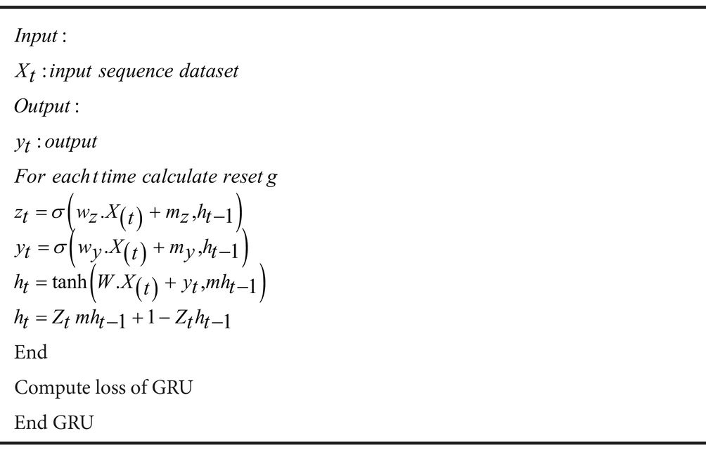
It is the kind of RNN (Recurrent Neural Network) method that tackles vanishing gradient problems and arrests long-term dependencies in sequential data. It is similar to the LSTM with fewer gradient mechanisms. The layers in the GRU method comprise the update gate, reset gate, and candidate state. The GRU model associating the input and forget gates into a distinct update gate and by a reset gate. The gating mechanism aid to handle the information flow by the network. It estimate that the information to maintain that to forget and encounter new information to include. Accordingly, the update gate defines the rate at the previous hidden state being upgraded and amount of new candidates added to the system. The reseat gate aids to decide how much information need to forget and the hidden state is restructured based on the update gate and reset gate. To enhance the performance of the proposed model by fine-tuning which altering the architecture and hyperparameter of the model. Hence, it led to enhanced generalization because, the fine tuning aids the proposed model to adjust better to the particular features of the dataset. Altering the learning rates can aid convergence of proposed model more efficiently and restricting overshooting the optimal solution. The performance of the proposed model is improve by the fine tune technique. It assists the method of deciding which is recollected and which is removed. Similarly, the reset gate is utilized to function the amount of the previously forgotten hidden state, and a new candidate is considered in the system. This reset data permits the selective reset of the hidden state regarding input data. Moreover, it permits the system to selectively reset the hidden state in terms of input. In the same way, the candidate state is composed of the hidden state where the input and reset gate capture the significant data from the present and preceding state. The Algorithm 2 explains the GRU mechanism.

Algorithm 2 Gated recurrent unit

Correspondingly, the presented system is further evaluated with the performance metrics to evaluate the efficacy of the classification.

4 Results and discussions

The section illustrates the outcome attained by the respective method. It signifies EDA, performance metrics, experimental results, comparative analysis, and performance analysis of the proposed method.

4.1 Exploratory data analysis

The EDA is used to view and analyze the data in the dataset. Figure 6 compares diverse gas emissions for top emitting countries.

Figure 6

Figure 6. Comparison of diverse gas emission for top emitting countries.

Figure 6 compares diverse gas emissions for top emitting countries. The Comparison of top countries which emits diverse gas emissions such as China, the European Union, Indonesia, Russia, and the United States. The analysis involves factors such as CH₄, CO₂, and N₂O. The analysis shows that the United States data contributes the highest CO₂ emission, and Indonesia has the lowest rate of CO₂ emission when compared with the other top countries.

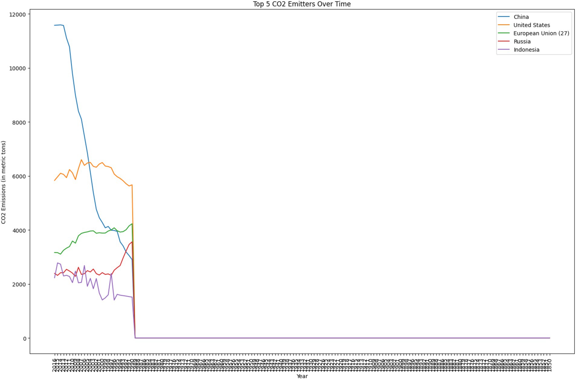
Accordingly, Figure 7 illustrates the top five emitters over time. The top five CO₂ emitters over time signifies that the emission of CO₂ in china is 12,000 tons, which is higher compared to the other countries.

Figure 7

Figure 7. Top five CO₂ emitters over time.

Congruently, Figure 8 represents the sum of emissions of each gas. The sum of emission of each gas illustrates the comparison of CH₄, N₂O, and CO₂. The analysis shows that CO₂ is the highest emission in all the top emission countries with 81.4% in China, 85.5% in the United States, 84.1% in the European Union, 79.2% in Russia and 69.8% in Indonesia. Accordingly, it is identified that the N₂O emission is limited when compared to the CH₄ and CO₂.

Figure 8

Figure 8. Sum of emission of each gas.

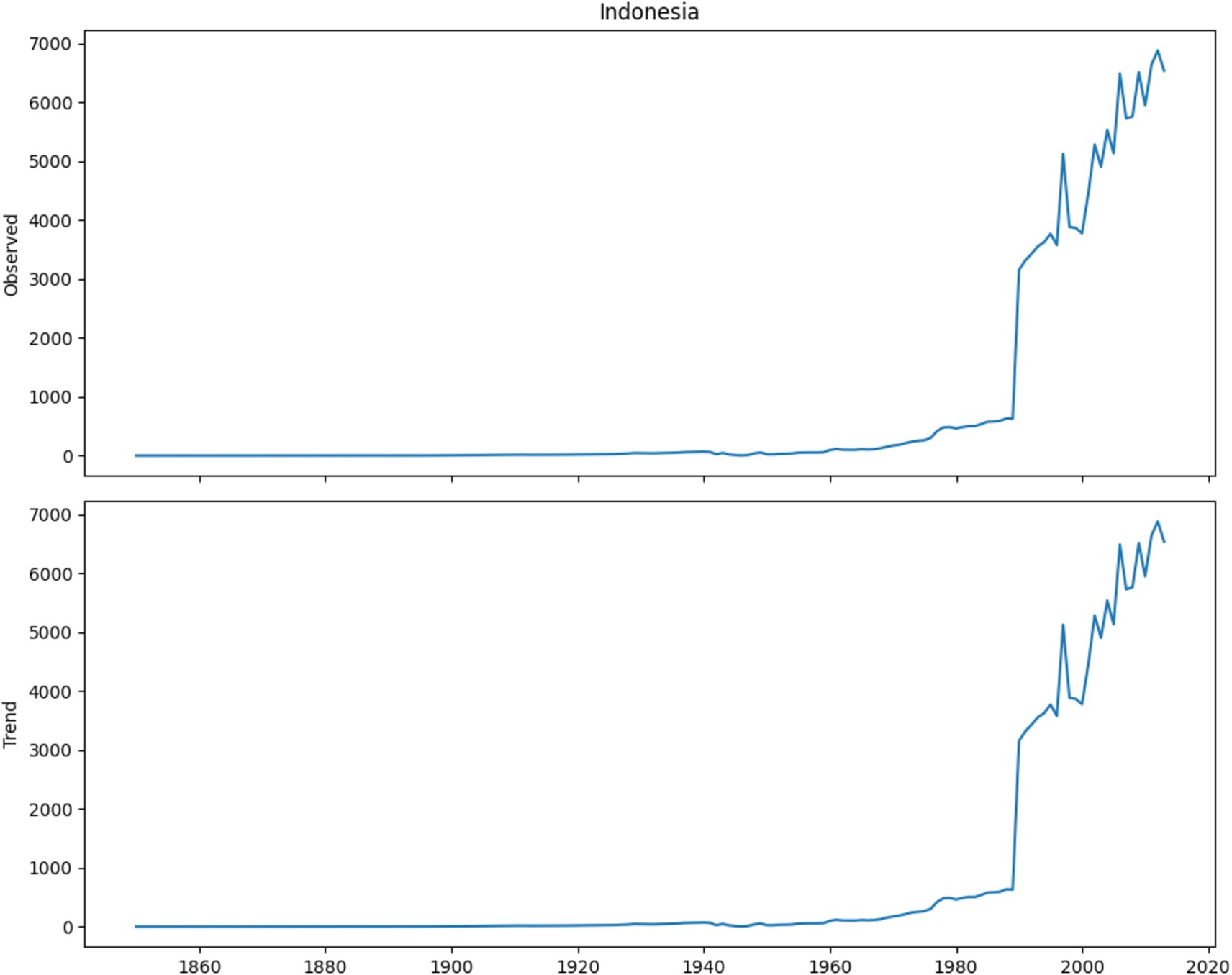
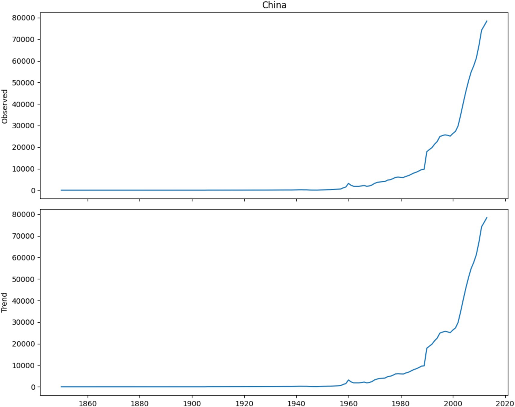
The Figures 9–13 shows the decomposition analysis for the countries such as Russia, Indonesia, China, European Union and United States. Wherein, the x-axis shows the year that ranges from 1860–2020, y-axis the emission trends, respectively. The Figures 9–13 describes the emission trends and observed values, where Russia emits 20,000 trends in the year 1960 and its observed graph is 20,000, for Indonesia the emission started at 1990 with 4,000 trends and it’s observed also shows 4,000. Similarly, China signifies the emission trends rises in the year 1990 with 40,000 and it attains peak value of 80,000 trends and observed in the year 2020. Moreover, for the European Union the emission is started in 1960 and it is identified in the year 1980–2020 with 30,000 trend and observed values. Whereas, United States has attained its highest emission in the year 2000 with 40,000 trend and observed and it is decreased from year 2000 to 2020.

Figure 9

Figure 9. Internal comparison of respective approach.

Figure 10

Figure 10. Internal comparison of respective approach.

Figure 11

Figure 11. Internal comparison of projected approach.

Figure 12

Figure 12. Internal comparison of presented approach.

Figure 13

Figure 13. Internal comparison of proposed approach (Rahman et al., 2023).

4.2 Performance metrics

The section represents the performance metrics utilized to calculate the efficiency of the respective research.

5 Mean square error

MSE is the measurement of image quality metric. If the values are closer to zero, the metric measurement is better in quality. This is obtained using Equation 21

$\begin{array}{ll}MSE=\frac{1}{n}{\displaystyle \sum }_{i=1}^n{\left(Y_i-Y_i\right)}^2& (21)\end{array}$

Here, the n signifies the number of data points, Yi denotes Observed values, and $\widehat{Y_i}$ is the predicted value.

6 Mean absolute error

The MAE measures the average magnitude of the errors in a set of forecasts among the paired observations used to express the same phenomenon without considering their direction. This parameter is also defined as the variance among the significant values present in the dataset and the projected values in the same dataset. This is obtained using Equation 22

$\begin{array}{ll}MAE={\displaystyle \sum }_{i=1}^n|y_i-x_i|/n& (22)\end{array}$

7 Root mean squared error

It is one of the common metrics utilized in the ML-based mechanism, which calculates the average difference between values in the prediction system and actual values. The Equation 23 represents the RMSE formula.

$\begin{array}{ll}\mathit{RMSE}=\sqrt{{\displaystyle \sum }_{i=1}^N{\left(\mathit{acutal}-\mathit{predicted}\right)}^2}/N& (23)\end{array}$

8 R–squared

The R-squared is the statistical calculation that signifies the proposition of variance for the dependent variable with the independent variable.

8.1 Experimental results

The section illustrates the outcome attained by the respective system.

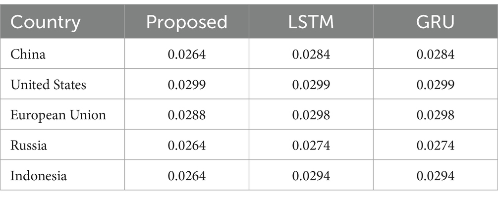
Table 1 and Figure 10 depicts the internal comparison proceeded in the proposed system with the classical algorithm. In the internal comparison, it is identified that the presented method attained an MAE value of 0.0264 for China, 0.0299 for the United States, 0.0288 for the European Union, 0.0264 for Russia, and 0.0264 for Indonesia. Here, it is revealed that the proposed approach accomplished better efficiency than the traditional model by attaining a minimum of 0.001 greater efficacy results with MAE value.

Table 1

Table 1. Internal comparison of respective system with MAE metric.

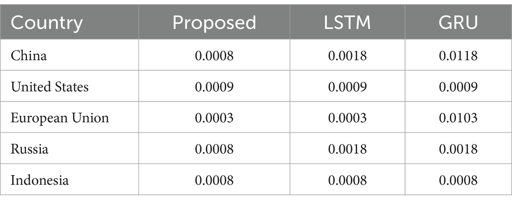
Table 2 and Figure 11 signify the internal comparison of the proposed system with the MSE metric. It is recognized that the presented method attained an MSE value of 0.0008 for China, 0.0009 for the United States, 0.0003 for the European Union, 0.0008 for Russia, and 0.0008 for Indonesia. Here, it is identified that the projected approach accomplished better efficiency than the pioneering model by attaining a minimum 0.00010 greater efficacy results with MSE value.

Table 2

Table 2. Internal comparison of projected system with MSE metric.

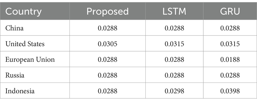
Table 3 and Figure 12 signify the internal comparison of the proposed system with the RMSE metric. It is identified that the respective method attained an RMSE value of 0.0288 for China, 0.0305 for the United States, 0.0288 for the European Union, 0.0288 for Russia, and 0.0288 for Indonesia. Here, it is identified that the proposed approach accomplished better efficiency than the classical model by attaining a minimum of 0.0010 greater efficacy results with RMSE value.

Table 3

Table 3. Internal comparison of presented system with RMSE metric.

8.2 Comparative analysis

The comparative analysis is carried out in the projected system to evaluate the performance of the respective research with the existing research.

The Table 4 and Figure 13 signifies the comparative analysis of the projected system with the classical model. The RMSE value for the proposed system is 0.0288, MAPE for the projected approach is 0.0007, and the R-Square value is 0.99. Besides, higher efficacy among the classical system is acquired from Feed Forward Neural Network where the projected approach accomplished 1.1012 with RMSE, 0.3893 with MAPE, 0.12 with R-square greater efficacy than the Feed Forward Neural Network results. Therefore, the outcome of the comparative analysis signifies the better efficacy of the presented system.

Table 4

Table 4. Comparative analysis of the projected system with conventional model (Rahman et al., 2023).

8.3 Performance analysis

The efficacy of the presented system is evaluated in this section. Figure 14 depicts the forecasting and loss value for the country China.

Figure 14

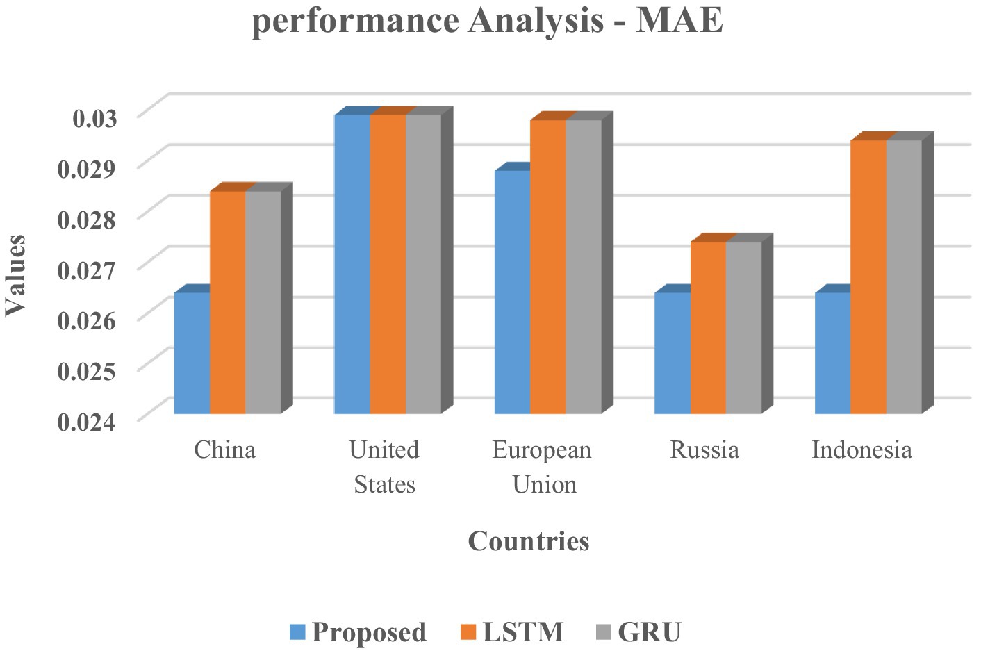
Figure 14. Forecasting and loss value for China, European Union, Indonesia, Russia and United States.

Figure 14 encapsulate emissions trends in addition to forecasting of different counties such as China, European Union, Indonesia, Russia and United States. Furthermore, China has attained highest emissions, trailed with measured progress with stability predictions. The European Union exhibited greater emissions initially and it increases gradually with the decrease in the forecast, along with substantial declination in training loss. Besides, Indonesia has established constant emissions through an insignificant escalation, which is predictable in the upcoming years. Accordingly, Russia’s emissions peaked formerly, but it is endured it steadiness for a period of time, then it is estimated to remain steady in advanced year. Moreover, United States had great emissions at the initial stage, and there is a declination and increase in the forecast in future. Generally, the Figure 14 emphasis trends of actual high emissions tailed by steadiness or reduction, together with enhanced forecasting precision through entire counties.

The proposed system utilized the advantages of configuration of a gating mechanism incorporating fine-tuning shifts in the Bi-LSTM-GRU algorithm to predict GHG emission in top emitting countries with the PRIMAP-host dataset obtained better results with higher efficiency which is identified through the results. Moreover, comparative analysis signifies that the proposed system outperforms the classical algorithms and existing research which is exposed through the outcome of internal and external comparison. Here, external comparison is performed with a single conventional model because the utilized dataset is limited in the classical approaches. For that reason internal comparison is performed in the presented system.

9 Conclusion

Globally, climate change is a crucial problem that affects the environment through various factors such as temperature rise, health effects, etc. Accordingly, GHG emission is the main factor that is responsible for climate change in the world. It is necessary to identify the GHG emission in the specific region to reduce the future consequences. Traditionally, identifying GHG emissions involves manually recognizing and quantifying the sources and amount of GHG released into the atmosphere. However, this manual identification process has several drawbacks, including being time-consuming, relying on limited resources, being prone to human error, and having limited scalability and coverage. To overcome these limitations, there is a need for a technology-based system that can effectively identify GHG emissions. To achieve this, several conventional researches attempted to attain better efficiency in the GHG emission but lacked accuracy issues, slower processing speed, and difficulty in handling larger datasets. To address the problem, the proposed research utilized the configuration of a gating mechanism incorporating fine-tuning shifts in the Bi-LSTM-GRU algorithm to predict GHG emission in top emitting countries with the PRIMAP-host dataset. Here, Bi-LSTM is used for the capability of capturing significant features, handling vanishing gradient problems, etc. On the contrary, it is lacking in long-term dependencies and overfitting. To tackle the issue, GRU is used with Bi-LSTM to enhance efficiency. This permits the proposed model to seizure setting from both earlier and future time steps. Due to this process in both directions, the BiLSTM understand the relationship in data. The integration of GRU aid for rapid training and decreased the danger of over fitting, particularly with smaller dataset by infusion of GRU in the input layer of BiLSTM with tuning process in the BiLSTM. Besides, the configuration of gates with fine-tuning shifts to improve the prediction performance. Moreover, the efficiency of the proposed method is calculated with performance metrics. The experimental results signify that the proposed system attained an MAE value of 0.0264 for China, 0.0299 for the US, 0.0288 for the EU, 0.0264 for Russia, and 0.0264 for Indonesia. Likewise, the internal comparative analysis shows that the respective model accomplished 0.002 MAE of higher efficiency classical LSTM and GRU methods. Similarly, the outcome of external comparative analysis signifies that the proposed method attained an RMSE of 1.1012, which is of greater efficacy than the existing systems. The selection of features in the proposed model can majorly affect the proposed model’s performance can give biased or incomplete predictions. In the future, using RFE (Recursive Feature Elimination) the significance of the feature will be analyzed to develop new features which seizure more related information.

Data availability statement

The original contributions presented in the study are included in the article/supplementary material, further inquiries can be directed to the corresponding author.

Author contributions

MS: Conceptualization, Funding acquisition, Methodology, Project administration, Software, Supervision, Validation, Writing – original draft. SE: Conceptualization, Data curation, Formal analysis, Investigation, Methodology, Validation, Visualization, Writing – review & editing. AB: Conceptualization, Data curation, Formal analysis, Investigation, Resources, Visualization, Writing – original draft. MM: Conceptualization, Data curation, Formal analysis, Investigation, Project administration, Resources, Software, Validation, Writing – review & editing.

Funding

The author(s) declare that financial support was received for the research, authorship, and/or publication of this article. This project is sponsored by Prince Sattam Bin Abdulaziz University (PSAU) as part of funding for its SDG Roadmap Research Funding Programme project number PSAU-2023-SDG-85.

Conflict of interest

The authors declare that the research was conducted in the absence of any commercial or financial relationships that could be construed as a potential conflict of interest.

Publisher’s note

All claims expressed in this article are solely those of the authors and do not necessarily represent those of their affiliated organizations, or those of the publisher, the editors and the reviewers. Any product that may be evaluated in this article, or claim that may be made by its manufacturer, is not guaranteed or endorsed by the publisher.

References

Aamir, M., Bazai, S. U., Marjan, S., Mirza, A. M., Wahid, A., Hasnain, A., et al. (2022). Predicting the Environmental Change of Carbon Emission Patterns in South Asia: A Deep Learning Approach Using BiLSTM. Atmosphere 13:2011. doi: 10.3390/atmos13122011

Crossref Full Text | Google Scholar

Abdul Latif, S. N., Chiong, M. S., Rajoo, S., Takada, A., Chun, Y. Y., Tahara, K., et al. (2021). The Trend and Status of Energy Resources and Greenhouse Gas Emissions in the Malaysia Power Generation Mix. Energies 14:2200. doi: 10.3390/en14082200

Crossref Full Text | Google Scholar

Adjuik, T. A., and Davis, S. C. (2022). Machine Learning Approach to Simulate Soil CO2 Fluxes under Cropping Systems. Agronomy 12:197. doi: 10.3390/agronomy12010197

Crossref Full Text | Google Scholar

Ajwang'Ondiek, R., Hayes, D. S., Kinyua, D. N., Kitaka, N., Lautsch, E., Mutuo, P., et al. (2021). Influence of land-use change and season on soil greenhouse gas emissions from a tropical wetland: A stepwise explorative assessment. Sci. Total Environ. 787:147701. doi: 10.1016/j.scitotenv.2021.147701

Crossref Full Text | Google Scholar

Aljughaiman, A. A., Cao, N. D., and Albarrak, M. S. (2024). The impact of greenhouse gas emission on corporate’s tail risk. J. Sustain. Finan. Invest. 14, 68–85. doi: 10.1080/20430795.2021.2012117

Crossref Full Text | Google Scholar

Al-Nefaie, A. H., and Aldhyani, T. H. J. S. (2023). Predicting CO2 emissions from traffic vehicles for sustainable and smart environment using a deep learning model. Sustain. For. 15:7615. doi: 10.3390/su15097615

Crossref Full Text | Google Scholar

Bakay, M. S., and Ağbulut, Ü. (2021). Electricity production based forecasting of greenhouse gas emissions in Turkey with deep learning, support vector machine and artificial neural network algorithms. J. Clean. Product. 285:125324. doi: 10.1016/j.jclepro.2020.125324

Crossref Full Text | Google Scholar

Biswas, S., Islam, M. S., Sarkar, S., and Rahman, R. (2021a). "Implementation of Machine Learning to estimate the measurement of air pollutants such as CO2, CH4, N2O, and total greenhouse gas emissions in Bangladesh."

Google Scholar

Biswas, S., Sarkar, S., and Islam, M. (2021b). Implementation of machine learning to estimate the air pollutants such as Carbon dioxide, methane, nitrous oxide and total greenhouse gas emissions in Bangladesh. Dhaka: Brac University.

Google Scholar

Casey, G. (2024). Energy efficiency and directed technical change: implications for climate change mitigation. Rev. Econ. Stud 91, 192–228. doi: 10.1093/restud/rdad001

Crossref Full Text | Google Scholar

Chang, W., Chen, X., He, Z., and Zhou, S. (2023). A Prediction Hybrid Framework for Air Quality Integrated with W-BiLSTM (PSO)-GRU and XGBoost Methods. Sustainability 15:16064. doi: 10.3390/su152216064

Crossref Full Text | Google Scholar

Ding, S., Hu, J., and Lin, Q. (2023). Accurate forecasts and comparative analysis of Chinese CO2 emissions using a superior time-delay grey model. Energy Econ. 126:107013. doi: 10.1016/j.eneco.2023.107013

Crossref Full Text | Google Scholar

Erdoğan, E., Serin Oktay, D., Manga, M., Bal, H., and Algan, N. (2024). Examining the Effects of Renewable Energy and Economic Growth on Carbon Emission in Canada: Evidence from the Nonlinear ARDL Approaches. Eval. Rev. 48, 63–89. doi: 10.1177/0193841X231166973

PubMed Abstract | Crossref Full Text | Google Scholar

Esparza-Gómez, J. M., Luque-Vega, L. F., Guerrero-Osuna, H. A., Carrasco-Navarro, R., García-Vázquez, F., Mata-Romero, M. E., et al. (2023). Long short-term memory recurrent neural network and extreme gradient boosting algorithms applied in a greenhouse’s internal temperature prediction. Appl. Sci. 13:12341. doi: 10.3390/app132212341

Crossref Full Text | Google Scholar

Faruque, M. O., Rabby, M. A. J., Hossain, M. A., Islam, M. R., Rashid, M. M. U., and Muyeen, S. (2022). A comparative analysis to forecast carbon dioxide emissions. Ener. Rep. 8, 8046–8060. doi: 10.1016/j.egyr.2022.06.025

Crossref Full Text | Google Scholar

Gong, L., Yu, M., Jiang, S., Cutsuridis, V., and Pearson, S. (2021). Deep Learning Based Prediction on Greenhouse Crop Yield Combined TCN and RNN. Sensors 21:4537. doi: 10.3390/s21134537

Crossref Full Text | Google Scholar

Hamrani, A., Akbarzadeh, A., and Madramootoo, C. A. (2020). Machine learning for predicting greenhouse gas emissions from agricultural soils. Sci Total Environ 741:140338. doi: 10.1016/j.scitotenv.2020.140338

Crossref Full Text | Google Scholar

Han, Z., Cui, B., Xu, L., Wang, J., and Guo, Z. (2023). Coupling LSTM and CNN neural networks for accurate carbon emission prediction in 30 Chinese provinces. Sustainability 15:13934. doi: 10.3390/su151813934

Crossref Full Text | Google Scholar

Hasan, M. M., and Chongbo, W. (2020). Estimating energy-related CO2 emission growth in Bangladesh: The LMDI decomposition method approach. Energy Strategy Rev. 32:100565. doi: 10.1016/j.esr.2020.100565

Crossref Full Text | Google Scholar

He, W., Li, J., Tang, Z., Wu, B., Luan, H., Chen, C., et al. (2020). A Novel Hybrid CNN-LSTM Scheme for Nitrogen Oxide Emission Prediction in FCC Unit. Math. Problems Eng. 2020:8071810. doi: 10.1155/2020/8071810

Crossref Full Text | Google Scholar

Hien, N. L. H., and Kor, A.-L. (2022). Analysis and prediction model of fuel consumption and carbon dioxide emissions of light-duty vehicles. Appl. Sci. 12:803. doi: 10.3390/app12020803

Crossref Full Text | Google Scholar

Hu, H., Chen, J., Zhou, F., Nie, M., Hou, D., Liu, H., et al. (2024). Relative increases in CH4 and CO2 emissions from wetlands under global warming dependent on soil carbon substrates. Nat. Geosci. 17, 26–31. doi: 10.1038/s41561-023-01345-6

Crossref Full Text | Google Scholar

Javanmard, M. E., and Ghaderi, S. F. (2022). A hybrid model with applying machine learning algorithms and optimization model to forecast greenhouse gas emissions with energy market data. Sustain. Cities Soc. 82:103886. doi: 10.1016/j.scs.2022.103886

Crossref Full Text | Google Scholar

Jongaramrungruang, S., Thorpe, A. K., Matheou, G., and Frankenberg, C. (2022). MethaNet–An AI-driven approach to quantifying methane point-source emission from high-resolution 2-D plume imagery. Remote Sens. Environ. 269:112809. doi: 10.1016/j.rse.2021.112809

Crossref Full Text | Google Scholar

Kim, H.-K., Song, C. K., Hong, S. C., Shin, M. H., Seo, J., Kim, S. K., et al. (2020). Source Characteristics of Atmospheric CO2 and CH4 in a Northeastern Highland Area of South Korea. Atmosphere 11:509. doi: 10.3390/atmos11050509

Crossref Full Text | Google Scholar

Kumar, A. K., Ritam, M., Han, L., Guo, S., and Chandra, R. (2022). Deep learning for predicting respiratory rate from biosignals. Comput. Biol. Med. 144:105338. doi: 10.1016/j.compbiomed.2022.105338

Crossref Full Text | Google Scholar

Kumari, S., and Singh, S. K. (2023). Machine learning-based time series models for effective CO2 emission prediction in India. Environ Sci Pollut Res Int. 30, 116601–116616. doi: 10.1007/s11356-022-21723-8

Crossref Full Text | Google Scholar

Li, F., Hu, Y., and Wang, L. (2022). Carbon emission prediction using CNN-LSTM. Int. J. Multidiscipl. Res. Public. 5, 30–35.

Google Scholar

Liu, Y., Li, D., Wan, S., Wang, F., Dou, W., Xu, X., et al. (2022). A long short‐term memory‐based model for greenhouse climate prediction. Int. J. Intell. Syst. 37, 135–151. doi: 10.1002/int.22620

Crossref Full Text | Google Scholar

Marquet, P. A., Buschmann, A. H., Corcoran, D., Díaz, P. A., Fuentes-Castillo, T., Garreaud, R., et al. (2024). “Global change and acceleration of anthropic pressures on Patagonian ecosystems” in Conservation in Chilean Patagonia: Assessing the State of Knowledge, Opportunities, and Challenges (Cham: Springer International Publishing Cham), 33–65.

Google Scholar

Namboori, S. (2020). Forecasting carbon dioxide emissions in the United States using machine learning. National College of Ireland: Dublin.

Google Scholar

Orazalin, N. S., Ntim, C. G., and Malagila, J. K. (2024). Board sustainability committees, climate change initiatives, carbon performance, and market value. Br. J. Manag. 35, 295–320. doi: 10.1111/1467-8551.12715

Crossref Full Text | Google Scholar

Patole, S. C. (2021). Time series forecasting of methane emissions from livestock using machine learning. National College of Ireland: Dublin.

Google Scholar

Pelster, D. E., Chantigny, M. H., Royer, I., Angers, D. A., Vanasse, A., and Research, T. (2021). Reduced tillage increased growing season N2O emissions from a fine but not a coarse textured soil under the cool, humid climate of eastern Canada. Soil Tillage Res 206:104833.

Google Scholar

Rahman, M. M., Shafiullah, M., Alam, M. S., Rahman, M. S., Alsanad, M. A., Islam, M. M., et al. (2023). Decision Tree-Based Ensemble Model for Predicting National Greenhouse Gas Emissions in Saudi Arabia. Appl Sci 13:3832. doi: 10.3390/app13063832

Crossref Full Text | Google Scholar

Ritchie, H., and Roser, M.. (2024). Co₂ Emissions. Our World In Data.

Google Scholar

Taylor, O., and Ezekiel, P. (2023). A model for forecasting air quality index in Port Harcourt Nigeria using Bi-LSTM algorithm. Machine Learn. doi: 10.48550/arXiv.2302.03930

Crossref Full Text | Google Scholar

Tol, R. (2024). A meta-analysis of the total economic impact of climate change. Energy Policy 185:113922. doi: 10.1016/j.enpol.2023.113922

Crossref Full Text | Google Scholar

Venkateshalu, S. G., and Deshpande, S. L. (2023). An optimized CNN GNR detector for methane gas detection from HSI raster data using feature variable. Int. J. Intel. Syst. Appl. Eng. 12, 635–643.

Google Scholar

Wang, J., and Azam, W. (2024). Natural resource scarcity, fossil fuel energy consumption, and total greenhouse gas emissions in top emitting countries. Geosci. Front. 15:101757. doi: 10.1016/j.gsf.2023.101757

Crossref Full Text | Google Scholar

Wen, L., and Cao, Y. (2020). Influencing factors analysis and forecasting of residential energy-related CO2 emissions utilizing optimized support vector machine. J. Clean. Product. 250:119492. doi: 10.1016/j.jclepro.2019.119492

Crossref Full Text | Google Scholar

Hastomo, W., Aini, N., Karno, A. S. B., and Rere, L. M. R. (2022). Metode Pembelajaran Mesin untuk Memprediksi Emisi Manure Management. JNTETI 11, 131–139. doi: 10.22146/jnteti.v11i2.2586

Crossref Full Text | Google Scholar

Yang, X., Xiong, J., du, T., Ju, X., Gan, Y., Li, S., et al. (2024). Diversifying crop rotation increases food production, reduces net greenhouse gas emissions and improves soil health. Nat. Commun. 15:198. doi: 10.1038/s41467-023-44464-9

PubMed Abstract | Crossref Full Text | Google Scholar

Yuan, K., Zhu, Q., Li, F., Riley, W. J., Torn, M., Chu, H., et al. (2022). Causality guided machine learning model on wetland CH4 emissions across global wetlands. Agric Forest Meteorol. 324:109115. doi: 10.1016/j.agrformet.2022.109115

Crossref Full Text | Google Scholar

Zha, W., Yuping, L., Yujin, W., Ruilan, L., Daolun, L., Shan, Y., et al. (2022). Forecasting monthly gas field production based on the CNN-LSTM model. Energy 260:124889. doi: 10.1016/j.energy.2022.124889

Crossref Full Text | Google Scholar