Heterogeneity of the diurnal cycle of precipitation in the Amazon Basin

The diurnal cycle of precipitation in the Amazon Basin (AB) is not homogeneous, varying in its intensity, time of occurrence of precipitation peaks and in the shape of its diurnal distribution. This study presents a seasonal characterization of the mean diurnal cycle of precipitation in the AB from IMERG Final Run (∆x = 0.1° and ∆t = 30 min) database from 2001 to 2020. Diurnal and semi-diurnal oscillations were studied by harmonics analysis, i.e., using the first and second harmonics, respectively. Harmonic metrics of normalized amplitude (A_N), phase and mean hourly precipitation rate were analyzed. The A_N showed pixels within the AB with bimodal/uniform or unimodal distribution associated with the occurrence of two peaks (or none) or a single peak during the day. The phase of the first harmonic shows the time of occurrence of the precipitation rates peaks, as well as the displacement of the precipitation systems. The regionalization of the diurnal cycle was performed using the K-Means technique, showing that AB presents six clusters along its domain based mainly on the phase of the first harmonic. The spatial configuration of clusters showed seasonal variation, being modulated by the South American Monsoon System and the large-scale mechanisms responsible for triggering convection. However, their intensity, the shape of the diurnal distribution and the timing of precipitation peaks are modulated by local factors.

1 Introduction

The diurnal cycle of precipitation in the Amazon Basin (AB) is of great interest because of its heterogeneous behavior and because its simulation continues to be one of the greatest challenges for state-of-the-art numerical weather and climate models. The diurnal cycle is the end result of a series of multiscale atmospheric processes that interact with each other in complex ways. In the particular case of the Amazon, the interaction between the atmosphere and the biosphere, the effects of the Atlantic and Pacific oceans, and the presence of the Andes Mountains are relevant aspects for the understanding of the formation of rain-producing systems. The main systems that organize precipitation in AB are Mesoscale Convective Systems (MCSs) (Nesbitt et al., 2006; Biasutti and Yuter, 2013), whose propagation and life cycle characteristics are linked to several factors, such as large-scale circulation, topography, surface heterogeneity, and thermally induced local circulations (Cohen et al., 1995; Anselmo et al., 2020; Rehbein et al., 2017; Rehbein, 2021). The characteristic of a heterogeneous surface of the AB makes the MCSs present heterogeneous characteristics, thus producing heterogeneity of the diurnal cycle in space–time, differing both in their intensity and in the time of occurrence of the peaks. For example, in the western part of AB, bounded by the Andes mountain range, the effect of topography generates strong horizontal and altitudinal gradients of precipitation (Junquas et al., 2018; Chavez and Takahashi, 2017; Espinoza et al., 2015; Espinoza et al., 2020; Ruiz-Hernández et al., 2021). In the central sector of AB, the urban effect of the city of Manaus, the presence of rivers and rainforest generate different diurnal cycles of precipitation (Silva et al., 2004; Angelis et al., 2004; dos Santos et al., 2014; Tanaka et al., 2014; Burleyson et al., 2016; Santos et al., 2019) as a function of thermally induced local circulations and water vapor availability associated with surface heterogeneity. It is evident that the diurnal cycle of precipitation is strongly linked to local factors in a given region (Yang and Slingo, 2001). However, large-scale mechanisms (Arraut et al., 2012) and their associated physical processes would also act as triggers to initiate convection and generate diurnal cycle variability in the AB (Poveda et al., 2005). For example, previous studies found that episodes of the Amazonian (Anselmo et al., 2020) and the South American (Marengo et al., 2004) low-level jets impact the diurnal cycle of precipitation through their influence on cloud clusters and the intensity of moisture flux in the central and southwestern Amazon, respectively.

One of the fundamental tests of the quality of numerical weather and climate model forecasts is their ability to reproduce the observed rainfall, its annual and seasonal cycle, its spatial distribution and, in particular, its diurnal cycle, since it is the end result of the interaction of multiple multi-scale physical processes. Watters et al. (2021) evaluated the global-scale diurnal cycle of precipitation reproduction performance of the Coupled Model Intercomparison Project Phase 6 (CMIP6) models and the ECMWF Reanalysis product (ERA5; Hersbach et al., 2020). They showed that the state-of-the-art CMIP6 models (with parameterization and explicit convection resolution) and the reanalysis product ERA5 still have significant differences in the representation of the diurnal cycle, both in intensity and phase. However, they showed that models that explicitly solve for convection perform better than models that use parameterizations. Paccini and Stevens (2023) show the simulation performance of the diurnal cycle of precipitation simulation of the numerical weather prediction model ICON (Icosahedral Nonhydrostatic, Zängl et al., 2015) and the CMIP6 ensemble at 180 km resolution. The authors showed that a better representation of precipitation is obtained with the explicit representation of convection, with increased spatial resolution and its relation to organized systems. However, the spatial resolution refinement experiment showed no significant improvement. Paccini and Stevens (2023) suggest that there are unresolved processes in their simulations that play an important role in the representation of the diurnal cycle. Important features found of the diurnal cycle of precipitation over the globe, both from observational and modeling studies, can be found in Watters et al. (2021, and references therein). In the work of Junquas et al. (2018) conducted mesoscale numerical modeling experiments over the Andes Central, showing the importance of topography and its physical processes that control the behavior of the diurnal cycle of precipitation. As shown in the papers cited above (and references therein), the diurnal cycle of precipitation is particularly relevant because it has a strong local connection to surface heterogeneities and depends on large-scale forcing. Both the bias in the diurnal cycle simulations and its phase error motivate the best possible documentation of this finest-scale regular mode.

Observational studies of the diurnal cycle of precipitation in the AB showed evidence of its heterogeneous character. Cutrim et al. (2000), Angelis et al. (2004), Webler et al. (2007), and Tanaka et al. (2014) through networks of weather stations showed differences in the diurnal cycle depending on its location, varying both in its intensity as well as in its phase, and showing a marked seasonality. Saraiva et al. (2016) using a network of meteorological radars showed variability in the AB sub-regions of the diurnal cycle of convective and stratiform clouds with respect to their times of greatest frequency of occurrence, and a marked seasonality. Using products derived by remote sensing, Paiva et al. (2011) and Nunes et al. (2016) showed differences of the diurnal cycle of convection in the AB, both in its intensity and phase. These cited studies show differences in the diurnal cycle of precipitation in the AB, and each of them had limitations related to a low density of weather stations, short time series or were conducted over small areas and focused on the effect of local factors. Furthermore, none of these articles present a detailed overview of the different diurnal cycles of precipitation that can be found throughout AB.

This paper aims to perform a seasonal regionalization of the diurnal cycle of precipitation throughout the AB and to suggest common causal mechanisms acting in each homogeneous cluster. The high spatio-temporal resolution (∆x = 0.1° and ∆t = 30 min) of the IMERG product data and the fact of generating precipitation estimates in grid format offer the opportunity to characterize and analyze the diurnal cycle of the precipitation in the AB from a detailed overview. Thus, the present study is the first to regionalize, characterize, describe and document the diurnal cycle of precipitation in the AB using high spatial and temporal resolution satellite data for a 20-year period. Therefore, this work provides a framework and a quantitative analysis of the heterogeneity of the diurnal cycle of precipitation over the AB that can be useful in the validation of numerical weather and climate forecasting models, in addition to other applications.

2 Data and methods

2.1 Study area

The study area is the Amazon Basin (AB, ~20°S-5°N/80°W-50°W) with an approximate extension of 6.1 × 10⁶ km² (ANA, 2014) and with its main river covering a total distance of 6,570 km (ANA, 2019) from its source in the snow-capped Mismi, in Arequipa (Peru), to its mouth in the Atlantic Ocean. The AB experiences an average annual discharge of 209.000 m³/s at its mouth (Molinier et al., 1996). Its large extension and complex river system make the AB the largest hydrological system in the world (Callède et al., 2004; Callède et al., 2010; Molinier et al., 1996). In addition, the AB is characterized by strong topographic gradients (especially in the Andes Mountains), areas of rainforest, grasslands, urban cities, agriculture and deforestation, characteristics that make the AB to be considered non-homogeneous (Figure 1).

Figure 1

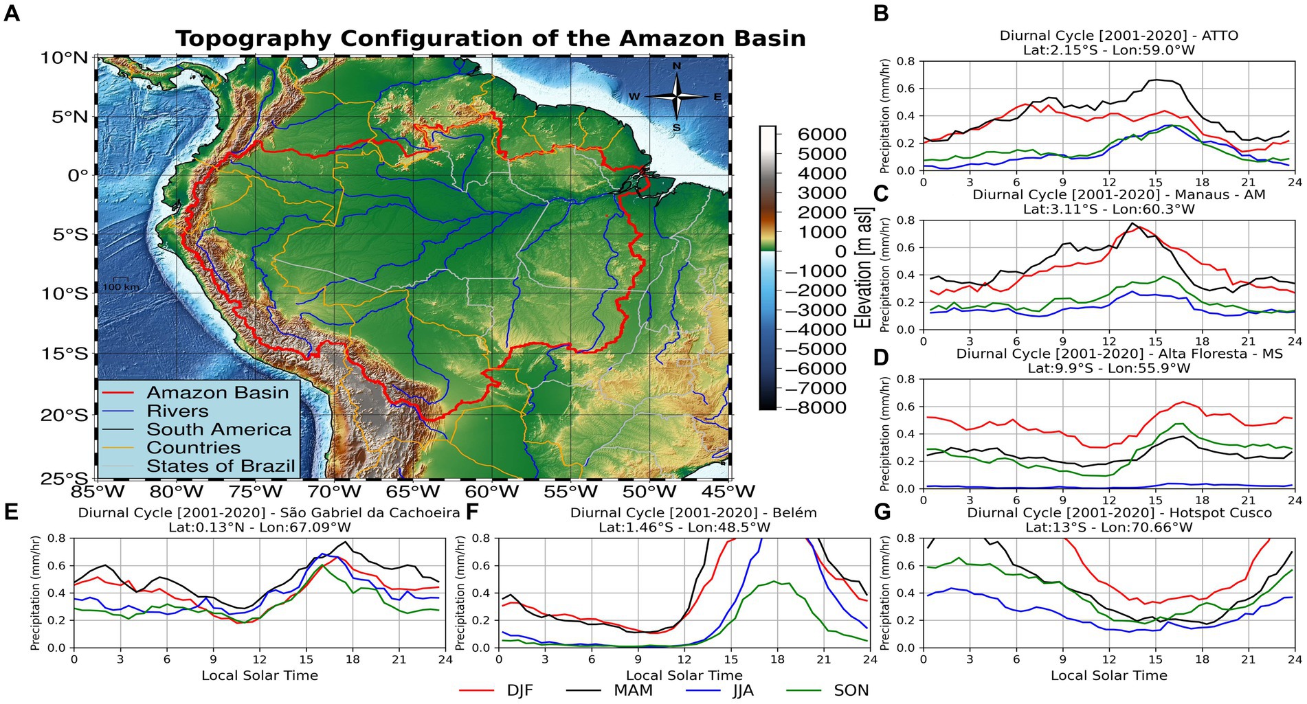
Figure 1. (A) The Amazon Basin (AB) topography (depicted in shades) with main rivers (blue lines), the red line is the outline of the AB, the gray line delimits the states of Brazil, the black line is the outline of South America and the symbols within the AB represent the locations from which the IMERG product precipitation rate time series shown in the panels were extracted. (B) Diurnal cycle of precipitation in ATTO (Amazon Tall Tower Observatory), (C) Manaus – AM, (D) Alta Floresta – MS, (E) São Gabriel da Cachoeira, (F) Belém, and (G) Hotspot Cusco. Curves represent the average diurnal cycle of precipitation for periods December to February – DJF (red), March to May – MAM (black), June to August – JJA (blue) and September to November – SON (green).

2.2 Precipitation data

The precipitation data for the study are from the Integrated Multi-satellitE Retrievals for the Global Precipitation Measurement (GPM) research product (IMERG, Huffman et al., 2019, 2020) for a 20-year period from 2001 to 2020. The IMERG product represents precipitation rate for each pixel with a spatial resolution of 0.1° x 0.1° and a temporal resolution of half an hour. Previous studies have shown that IMERG is a suitable product for analysis and monitoring of the diurnal cycle of precipitation globally (Tan et al., 2019; Watters and Battaglia, 2019; Watters et al., 2021). In the AB, Rehbein and Ambrizzi (2023) used IMERG data to study the behavior and life cycle of mesoscale convective systems (MCSs). Therefore, in this study we have considered the IMERG product as a suitable observational dataset for the analysis of the heterogeneity of the diurnal cycle of precipitation experienced by the AB.

2.3 Diurnal cycle of precipitation

Half-hourly precipitation rate data of IMERG from January 2001 to December 2020 were used to estimate the mean diurnal cycle in the AB. First, we calculated composites of precipitation rate for each time step (Equation 1) and for the seasonal periods December–January–February (DJF), March–April–May (MAM), June–July–August (JJA), and September–October–November (SON):

$\begin{array}{ll}P\left(\phi ,\lambda ,t_{UTC}\right)=\frac{{{\displaystyle \sum }}_{i=1}^{N}P{\left(\phi ,\lambda ,t_{UTC}\right)}_i}{N}& (1)\end{array}$

where N is the number of days of each seasonal period and P_i is the precipitation rate for a given latitude, longitude and time UTC. In this way, P represents forty-eight half-hourly observations of precipitation rate over a diurnal cycle starting at 0000 UTC. After that, the variability of diurnal cycle of precipitation was analyzed using harmonic analysis by first two harmonics, which means precipitation rate oscillations of 24 (first harmonic) and 12 (second harmonic) hours. For each pixel, the time series was represented as a harmonic function (Equation 2) using the methodology proposed by Wilks (2011):

$\begin{array}{ll}{Y}_t=\overline{Y}+{\displaystyle \sum _{k=1}^{n/2}}{C}_k\cos \left(\frac{2\pi tk}{n}-{\varphi }_k\right)& (2)\end{array}$

where $\overline{Y}$is the mean of the series (or fundamental harmonic), n is the sample size, C_k is the amplitude of harmonic k, Φ_k is the phase of harmonic k. To represent diurnal and semi-diurnal oscillations k is restricted to k = 1 e 2, respectively. Next, the amplitude for each harmonic C_k (Equation 3) is estimated by:

$\begin{array}{ll}{C}_k={\left[A_k^2+B_k^2\right]}^{0.5}& (3)\end{array}$

where coefficients of functions cosine (A_k) and sine (B_k) were estimated by were estimated by Equations 4, 5, respectively:

$\begin{array}{ll}{A}_k=\frac{2}{n}{\displaystyle \sum _{t=1}^n}{Y}_t\cos \left(\frac{2\pi tk}{n}\right)& (4)\end{array}$

$\begin{array}{ll}{B}_k=\frac{2}{n}{\displaystyle \sum _{t=1}^n}{Y}_t\sin \left(\frac{2\pi tk}{n}\right)& (5)\end{array}$

Finally, the phase for each harmonic were estimated by Equation (6):

$\begin{array}{ll}{\varphi }_k=\arctan \left(\frac{B_k}{A_k}\right),se{A}_k>0& (6.1)\end{array}$

$\begin{array}{ll}{\varphi }_k=\arctan \left(\frac{B_k}{A_k}\right)\pm \pi ,se{A}_k<0& (6.2)\end{array}$

$\begin{array}{ll}{\varphi }_k=\frac{\pi }{2},se{A}_k=0& (6.3)\end{array}$

For this study, we calculated for each pixel the normalized amplitude, i.e., ratio between the amplitude and the mean value (Equation 7):

$\begin{array}{ll}{A}_N=\frac{C_k}{\overline{Y}}& (7)\end{array}$

In the case of the first harmonic, we follow the criterion of Easterling and Robinson (1985) for the normalized amplitude (Table 1) which establishes the shape of the distribution of the diurnal cycle of precipitation (Figure 2) for each pixel. In fact, Figure 2A shows a bimodal diurnal distribution with two preferred times of peak occurrence (~01 and 14 LST). On the other hand, Figures 2B,C present a unimodal diurnal distribution with one preferred time of occurrence of the maximum of the precipitation rates (around 16 LST).

Table 1

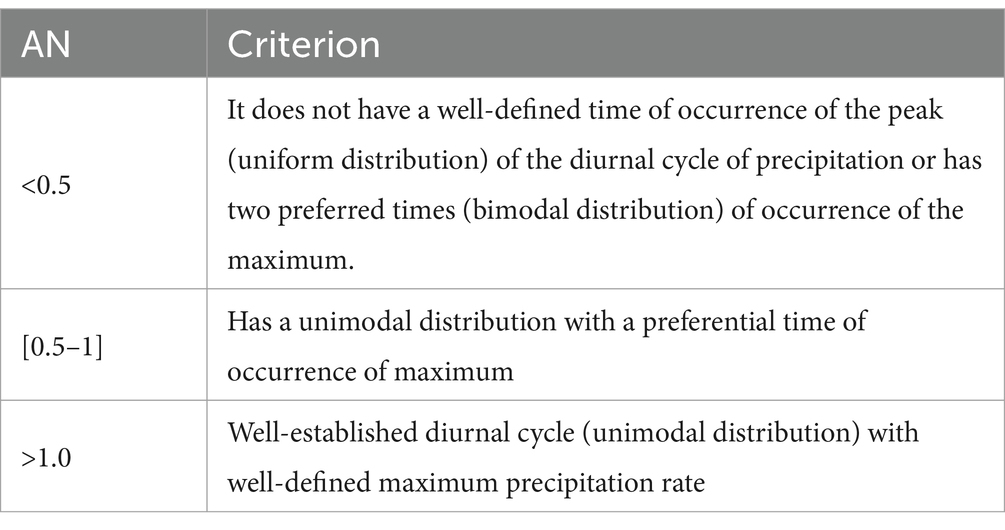
Table 1. Criterion of Easterling and Robinson (1985) for normalized amplitude of the first harmonic in the shape of the distribution of the diurnal cycle of precipitation.

Figure 2

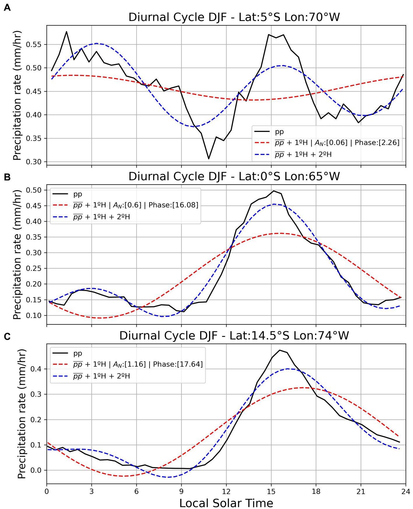
Figure 2. Distribution of the diurnal cycle of precipitation according to Easterling and Robinson (1985). (A) $A_N<0.5$, (B) $0.5⩽A_N⩽1.0$, and (C) $A_N>1.0$. In the three figures the red curve represents the mean precipitation rate + the 1° Harmonic (H), the blue curve represents the mean precipitation rate + 1°H + 2°H, and the black curve represents the mean precipitation rate for each time step.

The time at which the maximum precipitation rate occurs (Equation 8) is established when the argument of the cosine function is equal to zero as follows:

$\begin{array}{ll}{t}_{UTC}=\frac{\varphi n}{2\pi k}& (8)\end{array}$

We converted the time in UTC (t_UTC) to local solar time (t_LST) by Equation (9):

$\begin{array}{ll}{t}_{LST}=t_{UTC}+\frac{\lambda \left(°\right)}{15\left(°h^{-1}\right)}& (9)\end{array}$

where λ is the longitude in unit degrees. Therefore, when we refer to the hours of occurrence of maximum precipitation rates we use the LST format.

Finally, in this section we analyze harmonic metrics such as half-hourly mean precipitation rate, normalized amplitude and phase for the first two harmonics and associate their characteristics with the triggering mechanisms of convection in the Amazon Basin.

2.4 Cluster analysis

For the regionalization of the diurnal cycle of precipitation in the AB in homogeneous groups based on the harmonics metrics of the 24 and 12-h oscillations, we used the unsupervised “K-Means” (Wilks, 2011) clustering method. To use the K-Means algorithm, the dissimilarity measures and the number of k centroids must be specified for it to run and group regions with homogeneous diurnal cycles of precipitation. Once the dissimilarity measure and the number of k centroids have been determined, the first step is to randomly distribute the k centroids (elements representing the center of a cluster). The K-Means algorithm operates on a two-step process called expectation–maximization, where in the expectation step each element is attributed to its nearest centroid. Then in the maximization step, the mean of all the elements in each cluster is calculated and a new centroid is established. This process is repeated until the centroids converge or their position is the same as in the previous process. The quality of the clustering is determined by the sum of the squared error (SSE, Equation 10).

$\begin{array}{ll}{d}_{i,j}={\displaystyle \sum _{k=1}^k}{\left(x_{i,j}-x_{j,k}\right)}^2& (10)\end{array}$

Before applying the K-Means algorithm, we normalized each harmonic metric (half-hourly mean precipitation rate, normalized amplitude and phase for the first two harmonics) by dividing by the maximum value of each them. Next, we used the empirical orthogonal function (EOF, Lorenz, 1956) method to reduce the dimensionality of the harmonics metrics input dataset for each pixel within the AB and only used the first two principal components (PC1 and PC2). This means that we transform a high-dimensional dataset into a meaningful representation (PC1 and PC2) of lower dimension of it (Van Der Maaten et al., 2009). The measure of dissimilarity used in this study was Euclidean distances (Equation 11) which is determined as a distance in the space K-dimensionality between two vectors x_i e x_j (Wilks, 2011). The Euclidean distance is calculated by the following equation:

$\begin{array}{ll}{d}_{i,j}={\left[{\displaystyle \sum _{k=1}^k}\left(x_{i,j}-x_{j,k}\right)\right]}^{0.5}& (11)\end{array}$

where x_i e x_j are two vectors in the space K-dimensional (k = 1, 2, 3, …, K) (Wilks, 2011).

To determine the number of clusters (or centroids), we used two methods: the elbow method and the silhouette scores. Both methods use as input data the times series of PC1 and PC2. The elbow method is applied by running the K-Means algorithm several times increasing the number of clusters (or centroids) in each run and storing the SSE (Equation 10) values. Therefore, the number of clusters (k) is chosen according to the inflection point of the figure generated between the numbers of clusters (X-axis) and the SSE (Y-axis). Silhouette scores are based on two factors: (i) the proximity of the data element to other elements in the cluster, and (ii) the distance of the data element relative to the other elements in the other clusters. Silhouette scores (Equation 12) are calculated using the following equation:

$\begin{array}{ll}{S}_i=\frac{b\left(i\right)-a\left(i\right)}{\max \left\{a\left(i\right),b\left(i\right)\right\}}& (12)\end{array}$

where i is the analyzed element, a(i) is the average dissimilarity of the i-th element with the others elements of the same cluster, and b(i) is the average dissimilarity of the i-th element with all the elements of the nearest cluster (Rousseeuw, 1987). Silhouette coefficient values range from 1 to +1, with values close to +1 indicating that elements are closer to their clusters than to each other (Rousseeuw, 1987). Thus, the choice of the number of clusters was established by convergence of elbow method, silhouette scores and based on previous studies of regionalization of precipitation patterns in the AB (e.g., Sapucci et al., 2022; Ilbay-Yupa et al., 2021, Mayta et al., 2020; López, 2020; Saraiva et al., 2016; Nunes et al., 2016). Finally, we use the time series of the first two principal components and the number of clusters as input data to run the K-means algorithm.

We performed this methodology for each season of the year, i.e., DJF, MAM, JJA and SON in order to show that the diurnal cycle of precipitation in the AB is influenced by the seasonality of synoptic weather systems as well as by local factors. In addition, a time series analysis of each cluster is performed to demonstrate the heterogeneity of the diurnal cycles of precipitation experienced by each cluster as a function of seasonality and local factors. The flow chart of the methodology used in this work is shown in Figure 3.

Figure 3

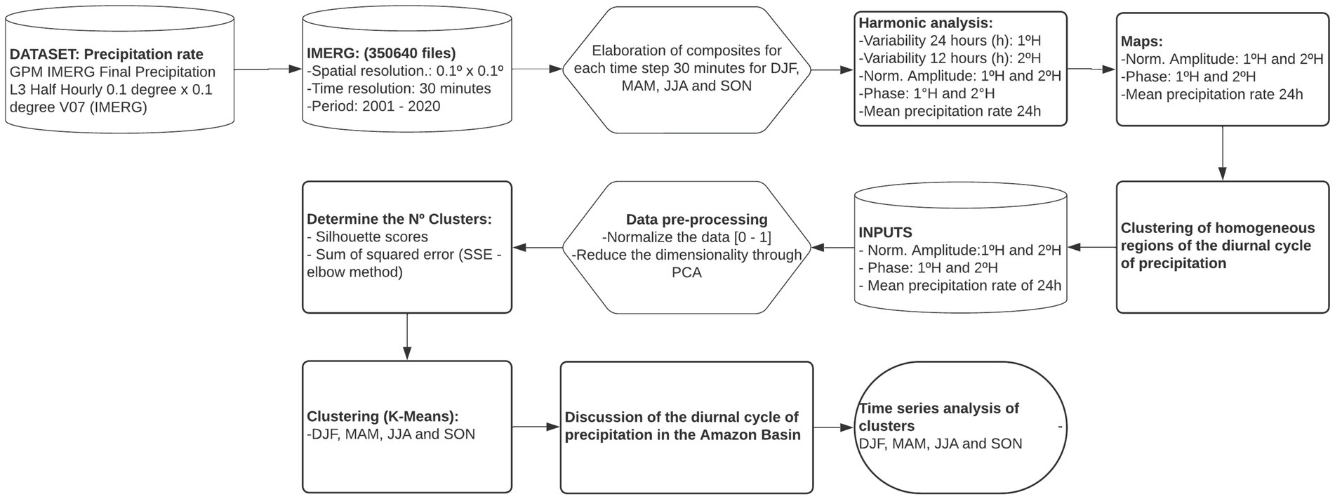
Figure 3. Schematic diagram of the methodology used in this work representing the steps from data collection to final results.

3 Results and discussions

3.1 Mean precipitation rate

Figure 4 shows a clear spatio-temporal variability of the mean hourly precipitation rate (mm/h, hereafter precipitation rate) across the Amazon Basin (AB) domain. Spatial variability is due to the heterogeneity of the surface with areas of the diverse rainforest, pastures, agriculture, rivers, the Andes mountain range and urban centers. These elements of the heterogeneity create thermally driven local circulations that interact with the large-scale circulation and depending on the availability of moisture inducing the formation of precipitation. The temporal variability shows a marked seasonality of the precipitation rate associated with the South American Monsoon System (SAMS, Vera et al., 2006) and large-scale mechanisms (Arraut et al., 2012; Fisch et al., 1998; Marengo and Nobre, 2009; Poveda et al., 2005; Satyamurty et al., 1998) responsible for the onset of convection. According to Nesbitt et al. (2006) the main systems that organize precipitation in the AB are the Mesoscale Convective Systems (MCSs). In this study, we used the 0.254 mm/h threshold (green colors in Figure 4) used in Rehbein et al. (2019) to associate precipitation rate with the occurrence of MCSs. The onset phase of the SAMS (Vera et al., 2006), is characterized by increased convection in the northwestern region of the AB and along the Andes around 1,500 meters (m) altitude. These regions of greater convective activity would be associated with the formation of MCSs, which are identified by precipitation rates greater than 0.254 mm/h. In this period (SON, Figure 4D) convection develops and moves toward the southeast region, thus favoring the production of precipitation. In the DJF period (Figure 4A), convective activity associated with MCSs are present in almost the AB (precipitation rate above 0.254 mm/h), except in the northernmost portion of the AB and in the high parts (above 1,500 m of altitude) of the Andes Mountain. This period (DJF) is associated with the mature phase of the SAMS (Vera et al., 2006) and is characterized by widespread convective activity in tropical South America. The MAM period (Figure 4B) is characterized by a decay phase of the SAMS (Vera et al., 2006) with convective activity moving northward. Precipitation rates associated with MCSs activity show a northward shift, being identified north of 10°S and around 1,500 m altitude in the Andes. The JJA quarter (Figure 4C) is characterized by the absence of SAMS. The convective activity is restricted to the northwestern and northern portion of the AB, with precipitation associated with the formation of MCSs (precipitation rate greater than 0.254 mm/h). In this period (JJA), the southeastern portion and the high parts of the Andes above 1,500 m present precipitation rates below 0.01 mm/h (Figure 4C, regions with crosses), indicating regions with scarce precipitation events.

Figure 4

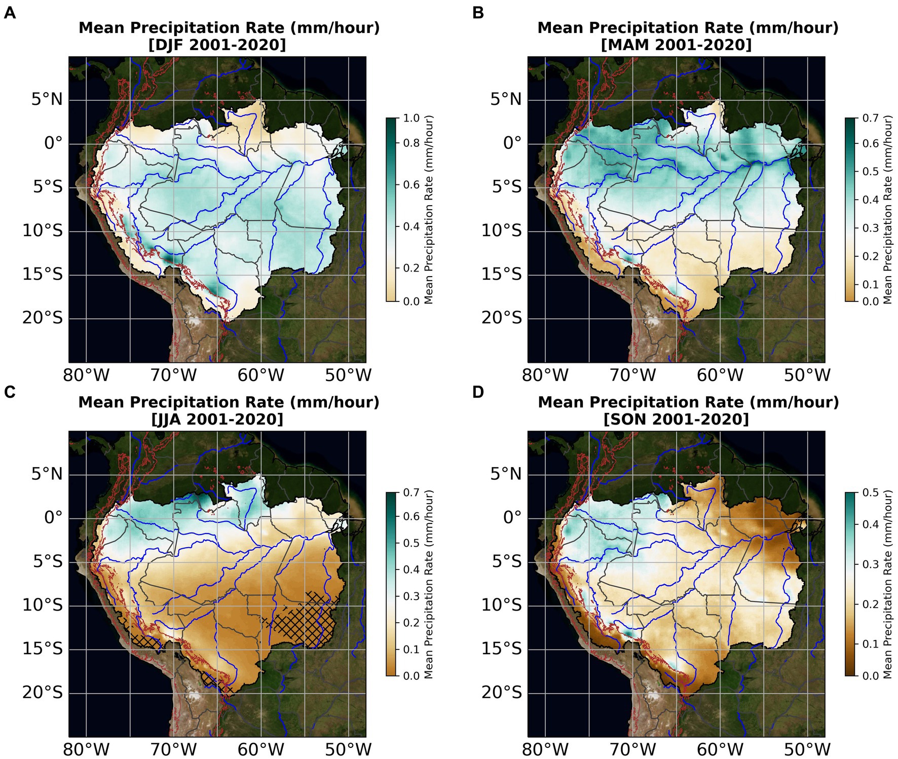
Figure 4. Mean precipitation rate (mm/h). (A) December–January–February (DJF), (B) March–April–May (MAM), (C) June–July–August (JJA), and (D) September–October–November (SON). The blue curve represents the main rivers of the Amazon Basin. The shades of green represent precipitation rate values above 0.254 mm/h. The regions with crosses “xx” cover areas in which the hourly mean precipitation rate is less than 0.01 mm/h. The brown line represents the elevation of the Andes at 1500 m a.s.l.

In addition, the precipitation rates show preferred regions of precipitation in the Andes, denominated precipitation hotspots (Chavez and Takahashi, 2017; Espinoza et al., 2015; Junquas et al., 2018), located in Bolivia and Peru. These precipitation hotspots have a marked seasonality, being more intense in the summer and less intense in the winter. Another significant aspect is observed along the Andean valleys of Peru (around 1,500 m of altitude) where there are centers of intense precipitation rates, showing a high spatial variability. This high spatial variability shows the strong precipitation gradients associated with the abrupt topography of the Andes (Espinoza et al., 2009; Espinoza et al., 2012; Figueroa and Nobre, 1990) creating thermally-driven local circulations and acting as a large-scale flow channelizer. Furthermore, the IMERG product detects intense precipitation rates near the main Amazon rivers, evidencing thermally-driven local circulations (river and land breezes). These regions with intense precipitation rates close to rivers present a marked seasonality and would be associated with flood periods of amazon rivers (dos Santos et al., 2014; Santos et al., 2019; Silva et al., 2004).

3.2 Normalized amplitude and phase of the first two harmonics

According to the criteria defined by Easterling and Robinson (1985) about the normalized amplitude of the first harmonic (hereafter A_N, Table 1), we have that if A_N is less than 0.5 (A_N < 0.5) the shape of the distribution of the diurnal cycle is uniform or bimodal. On the other hand, if A_N is greater than 0.5 (A_N > 0.5) the shape of the distribution of the diurnal cycle is unimodal. In this way, pixels with values of A_N < 0.5 present two preferred times of occurrence of precipitation peaks (bimodal distribution, Figure 2A) or do not present a preferred time of occurrence of precipitation peaks (uniform distribution, Figure 2A). Pixels with values of A_N > 0.5 show a single preferred time of occurrence of precipitation peaks (unimodal distribution, Figures 2B,C).

The spatial distribution of mean A_N calculated for the period 2001–2020 in the AB is shown in Figure 5 for each seasonal period. In Figure 5, pixels with values of A_N < 0.5 are represented with an orange gradient. On the other hand, values of A_N > 0.5 are represented with a violet gradient.

Figure 5

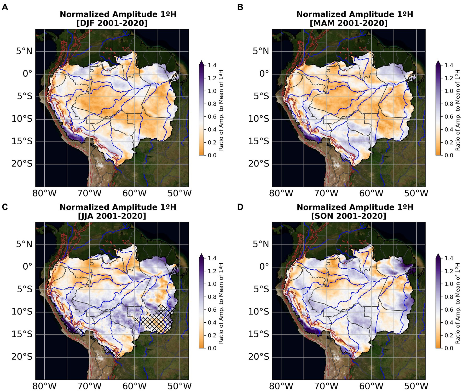
Figure 5. Normalized Amplitude 1°H. (A) December–January–February (DJF), (B) March–April–May (MAM), (C) June–July–August (JJA), and (D) September–October–November (SON). The blue curve represents the main rivers of the Amazon Basin. The regions with crosses “xx” cover areas in which the hourly mean precipitation rate is less than 0.01 mm/h. The shades of orange represent normalized amplitude values below 0.5 and shades of purple values above 0.5. The brown line represents the elevation of the Andes at 1500 m a.s.l.

Figure 6 shows the mean occurrence moments of the maximum hourly precipitation rates (phase) associated with diurnal oscillations (first harmonic) for each pixel over the AB calculated for the period 2001–2020. Times are defined in “Local Solar Times (LST)” format as follows: morning (06–12 LST), afternoon (12–18 LST), evening (18–24 LST) and dawn (00–06 LST).

Figure 6

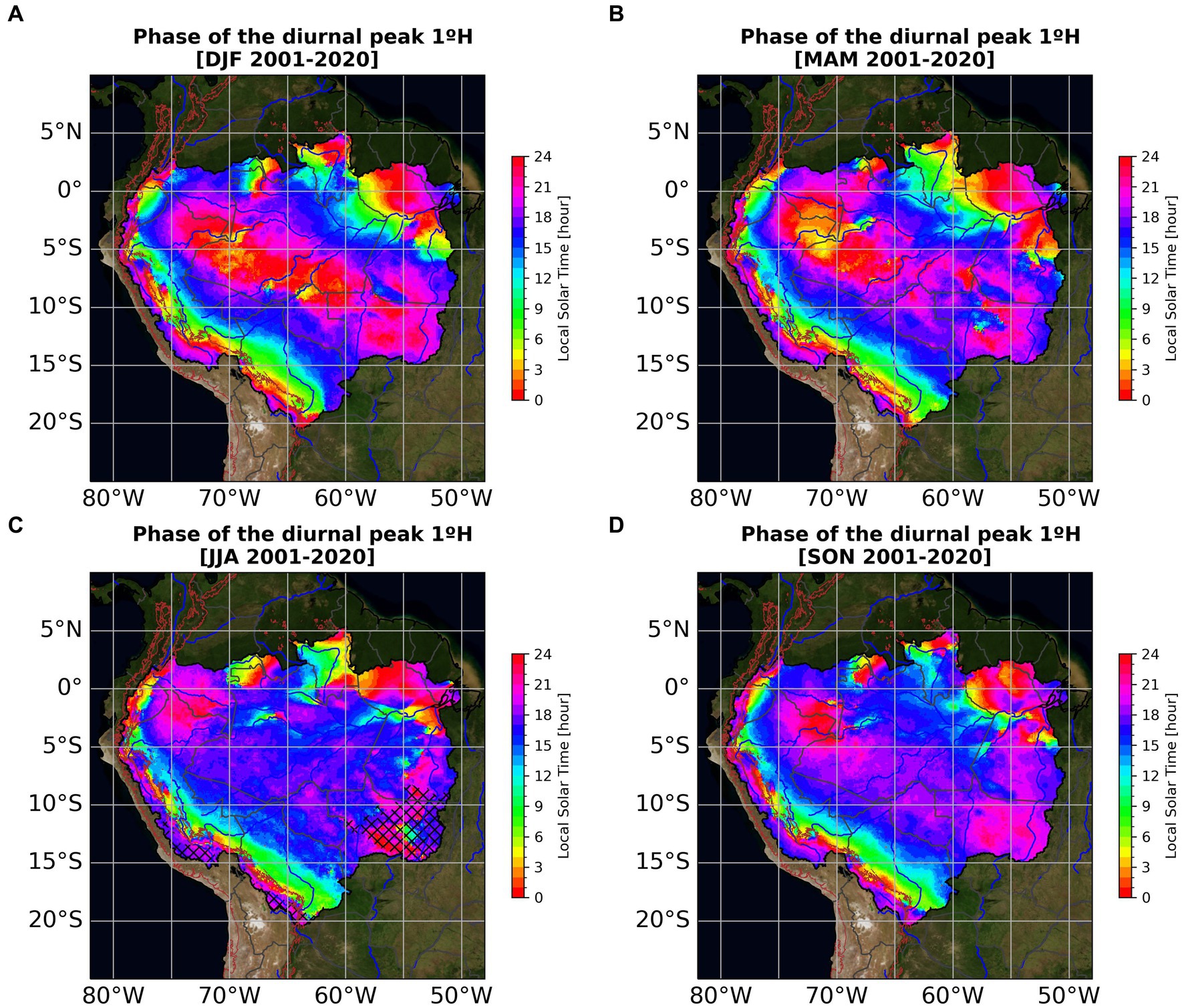
Figure 6. Phase of the time of occurrence (LST, Local Solar Time) of the peak of the 1°H oscillation. (A) December–January–February (DJF), (B) March–April–May (MAM), (C) June–July–August (JJA), and (D) September–October–November (SON). The blue curve represents the main rivers of the Amazon Basin. The regions with crosses “xx” cover areas in which the hourly mean precipitation rate is less than 0.01 mm/h. The brown line represents the elevation of the Andes at 1500 m a.s.l.

The normalized amplitude shows a seasonal behavior in the change of the spatial configuration of values lower than 0.5 (Figure 5). The seasonal spatial configuration of the A_N < 0.5 values present approximately the same spatial configuration of the seasonal mean density of the geometric centers of MCSs identified by Rehbein (2021, their Figure 8) and Rehbein et al. (2017, their Figure 5). These results suggest that values of A_N < 0.5 are associated with the precipitation signal generated by MCSs over the AB. Rao et al. (1996) highlight that in AB up to 65% of the total annual precipitation occurs between December to May, which is consistent with that shown in Figure 4, where the highest precipitation rates occur in the DJF (Figure 4A) and MAM (Figure 4B) periods. In this sense, the spatial distribution of A_N < 0.5 values would indicate that for the DJF and MAM periods, MCSs would be the main systems that organize precipitation in the AB (Nesbitt et al., 2006).

In Figure 5, the violet-colored pixel regions (A_N > 0.5) present a single precipitation peak of the diurnal cycle, which would be associated with the diurnal cycle of surface heating produced by radiative forcing, occurring generally in the afternoon (Figures 5, 6). Regions with orange pixels (A_N < 0.5) have two preferred times for the diurnal cycle peaks to occur, where a maximum usually occurs in the afternoon, associated with radiative forcing, and the second time occurs either at night, dawn or during the morning (Figures 5, 6). Thus, in Figure 6, the times of occurrence of the maximum precipitation rates (Figure 6) of the pixels with values of A_N < 0.5 correspond to the absolute maximum of their diurnal distributions.

Regarding the maximum that happens between night and morning, it may be associated to different forcing: (1) effect of local river breeze circulations (Cohen et al., 2014; dos Santos et al., 2014; Santos et al., 2019; Silva et al., 2004) or valley-mountain circulations (Ruiz-Hernández et al., 2021; Junquas et al., 2018), (2) episodes of the Amazonian Low Level Jet (ALLJ, Anselmo et al., 2020), (3) episodes of the South American Low-Level Jet (SALLJ, Marengo et al., 2004), (4) continent ward propagation of the sea breeze front (Burleyson et al., 2016), (5) life cycle and displacement of MCSs (Anselmo et al., 2021; Cohen et al., 1995; Rehbein, 2021) and (6) other mechanisms.

Furthermore, Figure 6 shows the diurnal displacement of the meteorological systems in the AB. For example, in the northeastern sector, the phase maps show the inland displacement in the AB of the systems that form in the northeastern coast of Brazil. Typically, the systems that form in this region are squall lines whose forcing is the sea breeze (Alcântara et al., 2011; Burleyson et al., 2016; Cohen et al., 1995; Janowiak et al., 2005). The squall lines reach their mature phase in the afternoon period and as they move inland they bring precipitation between late afternoon and evening (Figures 6A,B). Over this northeastern region, there is a double band with maximums occurring between the early morning and morning hours (yellow and green colors, respéctively) that would show the dissipation region of these systems. The dissipation of the squall lines bring moisture to the atmosphere and will serve as a source for the formation of new MCSs in the afternoon hours, which will continue their displacement toward the interior of the AB, a process that supports the hypothesis put forward in Anselmo et al. (2021). Similar processes occur on the western side of the AB (Figure 6), where a maximum occurs in the afternoon in the higher regions of the Andes Mountain, and as altitude decreases the maximums occur between night-dawn-morning. The mechanism that triggers the formation of precipitation in these regions is the valley-mountain breeze generated by differential heating between the valley and the slopes of the Andean mountains, with maximum heating in the afternoon hours on the slopes. At night-dawn-morning the process is reversed and we have a mountain-valley breeze, generating the displacement of the systems formed toward the east and southeast with the formation of new MCSs or with the intensification of the already existing ones. Here, we hypothesize that the region of maximum precipitation in the dawn-morning hours corresponds to a region of dissipation of the MCSs. This region will serve as a source of moisture that will then be used for the formation of new systems in the afternoon-night hours that will move toward the central region of the AB, where the maximums occur between night and dawn (Figures 6A,B). The central region of the AB presents precipitation peaks at night-morning (Figures 6A,B), probably because it is the region of convergence of the systems that systematically move from east to west (east side of the AB) and from west to east (west side of the AB). In addition, this region presents several mechanisms that will serve as triggers to active convection, e.g., nocturnal river breezes (Cohen et al., 2014; dos Santos et al., 2014; Santos et al., 2019; Silva et al., 2004), nocturnal episodes of ALLJ (Anselmo et al., 2020) and SALLJ (Marengo et al., 2004) and others. The JJA (Figure 6C) and SON (Figure 6D) periods present mainly precipitation peaks in the afternoon hours, with the main mechanism of convection activation being radiative forcing of the surface. The JJA period (Figure 6C) presents large-scale mechanisms that generate subsidence (Espinoza et al., 2013) and, therefore inhibit rainfall formation, which is why some regions present scarce rainfall (marked regions with crosses). During these periods, the northernmost region of the AB experiences precipitation due to the ingress of squall lines formed in the extreme north of South America, the mechanism of formation being a combination of the sea breeze and lifting of the air due to the topographic barrier of the Guiana shield (Alcântara et al., 2011; Cohen et al., 1995).

The normalized amplitude of the 2°H (see Supplementary material) is related to the semidiurnal variability, being bimodal when it is greater than the amplitude of the 1°H; otherwise, it will be unimodal. For the A_N of the 2°H there is no direct criterion to identify whether the distribution is unimodal or bimodal as in the case of the A_N of the 1°H (Easterling and Robinson, 1985, see Table 1). However, the relative difference (see Supplementary material) can be used, which is calculated as the difference between the amplitude of the first (C₁) and second (C₂) harmonics, normalized by the first harmonic and multiplied by 100. Positive values will indicate a unimodal dominant regime, while negative values will indicate a bimodal dominant regime. Regions with a greater contribution of the A_N of the 2°H than the A_N of the 1°H show that they are influenced by mechanisms that trigger convection at different times of the day (e.g., surface heating during the day and nocturnal episodes of the ALLJ favoring the formation of MCSs). On the other hand, These regions could receive precipitation contributions from systems in other regions at a certain time of the day (e.g., the passage of a squall line from the Atlantic coast in its dissipation stage in the northeastern region of AB, contributing light precipitation during the night). Additionally, one mechanism may trigger convection (surface heating generating thermally induced mesoscale circulations during the afternoon) at another time of day [as discussed in Hayden et al., 2023 in their Figure 10], but these two precipitation peaks do not necessarily occur on the same day. The uniform distribution can likely be identified in regions where the A_N of the 1°H and 2°H are very close and below 0.5, resulting in a smoothed wave without prominent peaks. This can probably be observed in the northwest of the AB, where precipitation can occur at any time of the day due to the high humidity and latent heat release experienced in this region.

The harmonic parameters (precipitation rate, normalized amplitude and phase) show that local factors such as the presence of rivers, orientation of mountain barriers, different land use and land cover, urbanized cities, play an important role as triggers of the heterogeneous diurnal cycle in the AB. Likewise, the seasonality of some of these factors (e.g., seasonality of river flooding periods, seasonality of the rainforest fire period, and others) contribute temporal and spatial variability to the diurnal cycle of precipitation in the AB, and motivate the development of more specialized research to better understand their role as triggers.

3.3 Regionalization of the diurnal cycle of precipitation in the Amazon Basin

3.3.1 Determining of the number of clusters of the diurnal cycle of precipitation

Figure 7 shows the results of the application of the silhouette scores (left) and elbow (right) methods, where for the periods DJF, MAM and JJA (Figures 7A–C, respectively) the number of clusters chosen was six. For the SON period (Figure 7D) the choice of the number of clusters was set to seven. The silhouette scores for the DJF, MAM and JJA periods with six clusters (seven for the SON period) show that they are higher than the mean value of the silhouette coefficient (dashed line in red, around 0.4). In addition, for the number of clusters established for each period, the silhouette shapes are relatively homogeneous in thickness. The elbow method shows that for DJF, MAM and JJA periods (Figures 7A–C) the SSE increases abruptly from six clusters (red dashed lines), while for the SON period (Figure 7D) it does so for seven clusters (red dashed line).

Figure 7

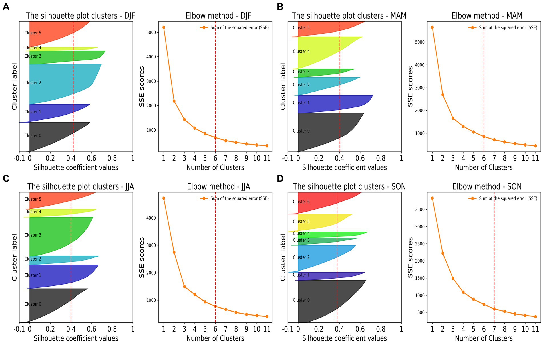
Figure 7. Silhouette (left) and elbow (right) method scores for the periods of (A) December–January–February (DJF), (B) March–April–May (MAM), (C) June–July–August (JJA), and (D) September–October–November (SON). The red lines of the silhouette coefficients indicate the mean value of the silhouette coefficient as a function of the number of clusters, and in the elbow method they represent the SSE value as a function of a given number of clusters.

Since the K-Means algorithm performs a clustering based on the similarity between elements through a distance function (here the metric used is the Euclidean distance), it is necessary to reduce the degrees of freedom of each element. To reduce the dimensionality (degrees freedom) of each element within the AB represented by the six harmonic parameters (mean precipitation rate, normalized amplitude and phase of the first two harmonics – the second harmonic shows two phases in a 24-h period), the principal component analysis (PCA) technique was applied. The first two principal components (PC1 and PC2) were obtained for each period, representing 56.8 and 20.5% for DJF, 49.5 and 25.9% for MAM, 42 and 28.1% for JJA, and 42.2 and 29.9% for SON, of the total variance, respectively. The PCA shows that the criterion of non-overlapping convex hulls is almost satisfied, being that where there is an overlap of the elements between different groups, it would represent the transition region between different behaviors of the diurnal cycle (Figure 8).

Figure 8

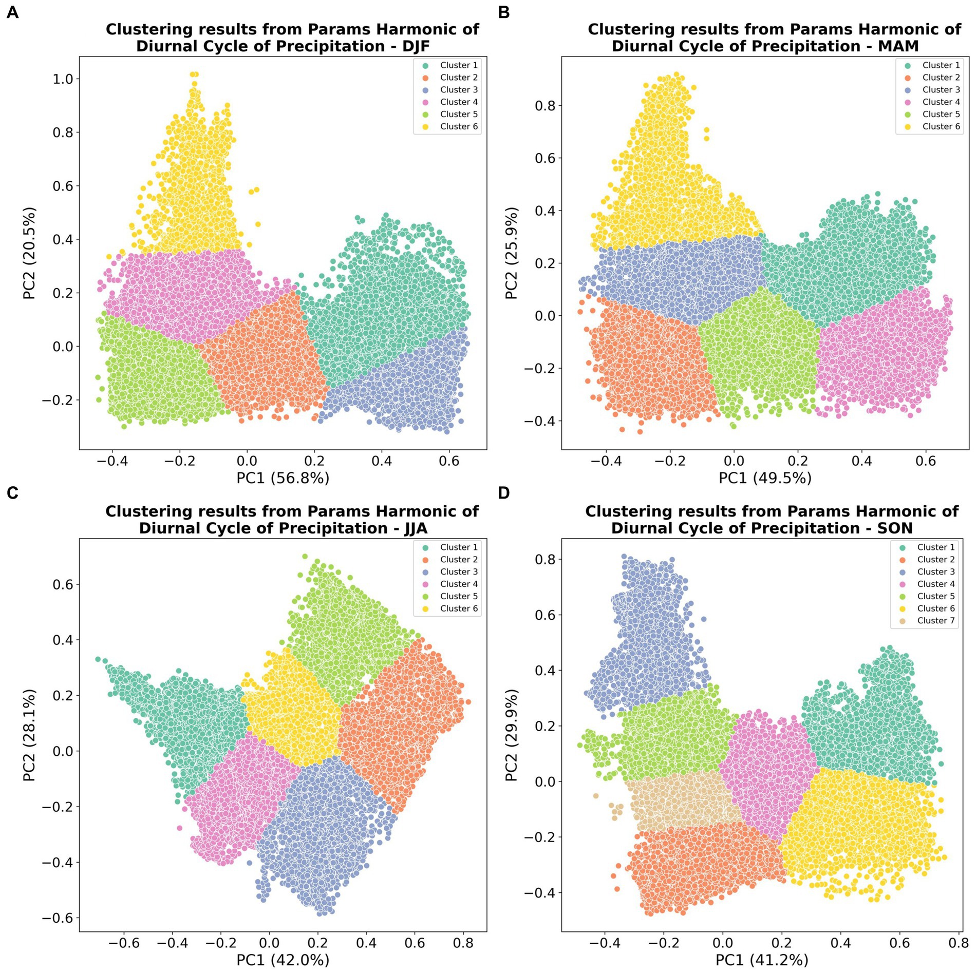
Figure 8. Representation of the clusters of the diurnal cycles in the space of the principal components (PC1 and PC2) estimated using the harmonic parameters for the periods of (A) December–January–February (DJF), (B) March–April–May (MAM), (C) June–July–August (JJA), and (D) September–October–November (SON).

3.3.2 Heterogeneity of the diurnal cycle of precipitation in the Amazon Basin

Figure 9 shows the spatial distribution of the different diurnal cycles of the precipitation (clusters) in the BA for the DJF, MAM, JJA and SON periods (Figures 9A–D). In the maps in Figure 9, black stars indicate pixels with normalized amplitude greater than 0.5 (A_N > 0.5), i.e., pixels with a unimodal diurnal distribution with a single preferred time of occurrence of the peak precipitation rate. On the other hand, pixels without black stars indicate normalized amplitude values lower than 0.5 (A_N < 0.5), i.e., pixels with a bimodal diurnal distribution (two peaks) or have a uniform distribution throughout the day.

Figure 9

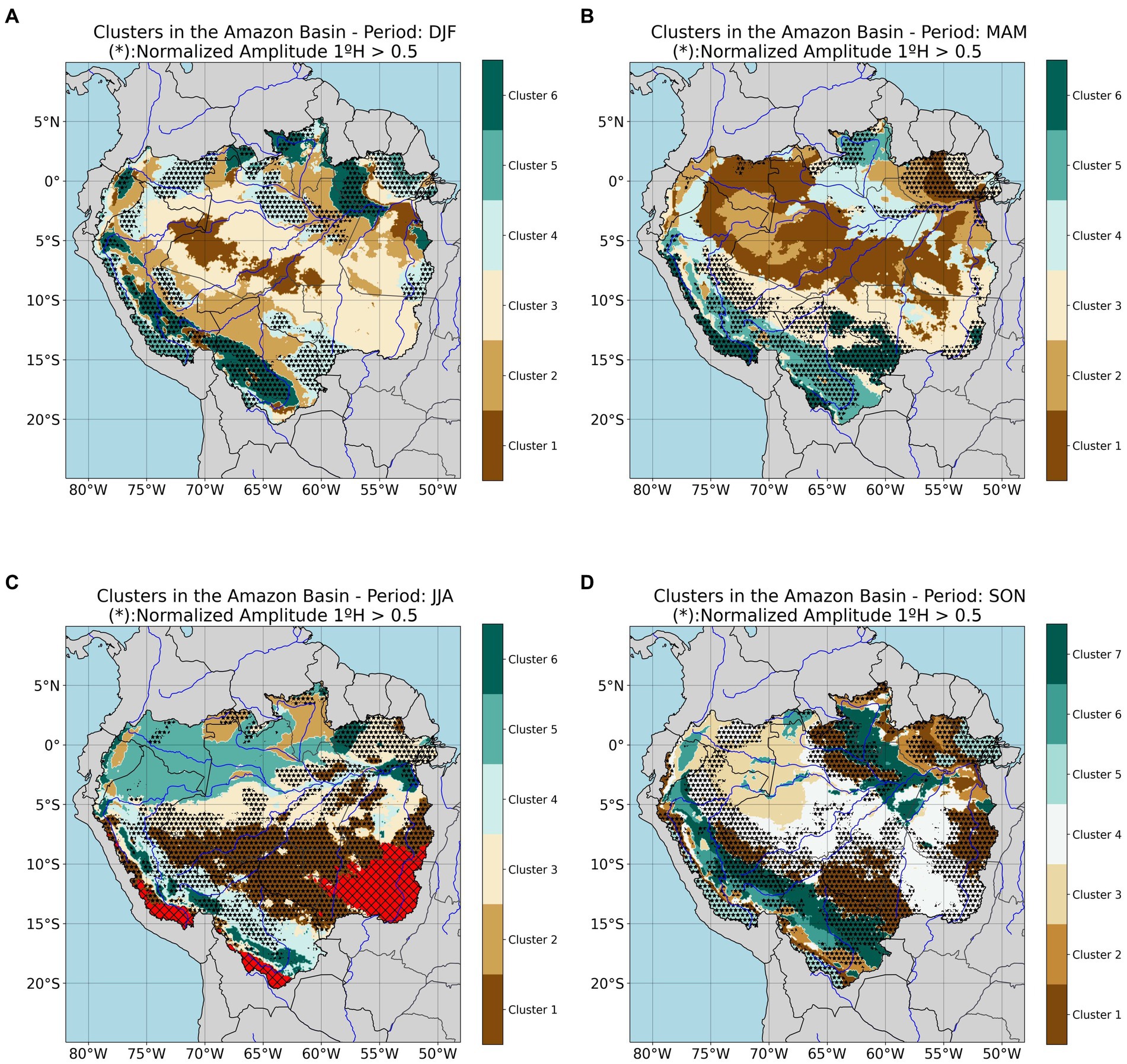
Figure 9. Spatial distribution of clusters (colors) of the diurnal cycle of precipitation in the Amazon basin for the periods of (A) December–January–February (DJF), (B) March–April–May (MAM), (C) June–July–August (JJA), and (D) September–October–November (SON). Black stars indicate $A_N>0.5$. The blue curves represent the main rivers of the AB. Red areas with crosses “xx” indicate regions with weak diurnal signals (mean precipitation rate < 0.01 mm/h).

3.3.2.1 December–January–February (DJF)

In the DJF period (Figure 9A) the AB has six different types of diurnal cycles (clusters). Black stars (A_N > 0.5) indicate that clusters 4, 5, and 6 (shades of green) exhibit a unimodal diurnal cycle, with a single peak of the mean precipitation rate (one predominant hour of peak occurrence). Cluster 4 presents exceptions in its unimodal behavior along the Andes mountain range in Bolivia, Ecuador and Peru (above 2000 meters altitude), and also in Colombia, where the normalized amplitude is less than 0.5 (A_N < 0.5). On the other hand, cluster 1 (brown), cluster 2 (mustard) and cluster 3 (yellow) are groups with a bimodal (or uniform) diurnal distribution characterized by two predominant times of peak occurrence (or no predominant times). Cluster 2 shows an exception to the bimodal or uniform behavior (A_N > 0.5) along the Amazon River near the Manaus region, experiencing a peak of the diurnal cycle in the afternoon (Figure 6), probably being induced by the urban factor. Cluster-1 and cluster-3 present an extension from northeastern Peru in the Loreto region to southeastern of the AB (Tocantis, Brazil), similar to the climatological configuration for this period of the South Atlantic Convergence Zone (SACZ, Carvalho et al., 2002, 2011). The northwest-southeast configuration of cluster-1 and cluster-3 is also associated with the systematic displacement of cloud systems from east to west.

3.3.2.2 March–April–May (MAM)

In the MAM period (Figure 9B) the AB was regionalized into 6 different types of clusters. The spatial configuration of the distribution of the different clusters is similar to the DJF period, but presents differences in the behavior of the diurnal cycle within the same cluster, e.g., a well-marked unimodal diurnal cycle near the Amazon River. Unlike the DJF period, in the MAM period a given cluster may have a unimodal diurnal distribution in one region and a bimodal/uniform distribution in another. For example, it is observed that in the northeastern region, clusters-1, cluster-2 and cluster-3 present a single predominant time of occurrence of precipitation rate peaks (unimodal distribution, A_N > 0.5). However, in the central region of the AB, these same clusters present two predominant times of peak occurrence, but with the absolute peak occurring at the same time (cluster-1 at night, cluster-2 in the early morning and cluster-3 in the afternoon, see Figure 6). Another interesting feature is the unimodal behavior (A_N > 0.5) of the diurnal cycle along the Amazon River of the cluster-4, but with a bimodal behavior away from the river. This different behavior within the same cluster-4 would indicate that the diurnal cycle is influenced by local factors (surface heterogeneity) (Yang and Slingo, 2001). In this period, cluster-1, cluster-2 and cluster-3 present a northwest-southeast spatial configuration similar to the climatological configuration of the SACZ (Carvalho et al., 2002, 2011) and associated with the systematic displacement of cloud systems in the east–west direction.

3.3.2.3 June–July–August (JJA)

In the JJA period the AB was divided into six different types of diurnal cycles (Figure 9C). In this period it is observed that the clusters south of 5°S present A_N values higher than 0.5 (black stars), indicating a unimodal behavior of the diurnal cycle, and the same behavior is observed in the northeastern region of the CA and in the northernmost parts. North of 5°S, in the northern and northwestern sector, clusters-2, cluster-5 and cluster-6 show a bimodal (or uniform) behavior of the diurnal cycle of precipitation (AN<0.5). Sectors with weak diurnal precipitation signals (precipitation rate < 0.01 mm/h, see Figure 4C) are colored red with crosses, representing dry regions or regions experiencing scarce precipitation events. These red areas are located in the southeastern and southern sectors and in the high parts of the Andes Mountains (southwest) of the AB. An interesting detail, observed north of 5°S, over the Amazon River, is that cluster-2 is differentiated within cluster-5. A similar behavior is observed along the Amazon river (cluster-4, formed by the confluence of the Solimões and Negro rivers) and over the urban city of Manaus (cluster-1) differing from cluster-3. This behavior highlights that local factors such as the presence of a river are determinant in modulating the characteristics of the diurnal cycle (Yang and Slingo, 2001).

3.3.2.4 September–October–November (SON)

Unlike the other study periods, in the SON period (Figure 9D) the AB was regionalized with 7 different types of clusters. The spatial configuration of the cluster distribution is similar to the DJF period (Figure 9A), probably associated with the seasonality of the onset of SAMS (Carvalho et al., 2002; Vera et al., 2006). Cluster-3 and cluster-4 configure a diagonal band with a northwest-southeast extension, similar to the climatological configuration of the SACZ (Carvalho et al., 2004, 2011). Much of the AB presents values of A_N > 0.5 indicating a predominant unimodal distribution of the diurnal cycle of precipitation for this period. The northeastern regions of Peru (Loreto) and northwestern Brazil (central AB) are characterized by a predominant bimodal/uniform distribution of precipitation (A_N < 0.5). In these regions mentioned above, it is observed that cluster-6 is formed on the Amazonian rivers, differentiating it from cluster-3, once again local factors are predominantly associated with the behavior of the diurnal cycle (Yang and Slingo, 2001).

In the four periods, it is observed that along the Andes Mountains and the transition zone between the Andean region and the Amazon forest there is a greater heterogeneity of clusters. This greater differentiation over relatively short distances is associated with the strong influence of local factors such as topographic gradients and different surface use and cover (Yang and Slingo, 2001). It is observed that the characteristics that predominated in the regionalization of the diurnal cycle were the normalized amplitude and the 1°H phase, the latter being the most influential. The fact that the 1°H phase is the most predominant feature in the regionalization explains why there are equal clusters in different sectors of the AB, e.g., in the DJF period cluster-6 is located northeast of the AB and along the Andes.

3.3.3 Analysis of time series

Figure 10 shows the time series of the different clusters for the four study periods for the central region of the AB (10°S-0°/70°W-50°W). Time series for the other AB regions are available in the Supplementary material, as well as short videos of the mean diurnal cycle for the entire CA and its regions. Information on the number and type of clusters per period for each AB’s region is summarized in tables in the Supplementary material, as well as the main meteorological systems acting in each region according to the literature available so far.

Figure 10

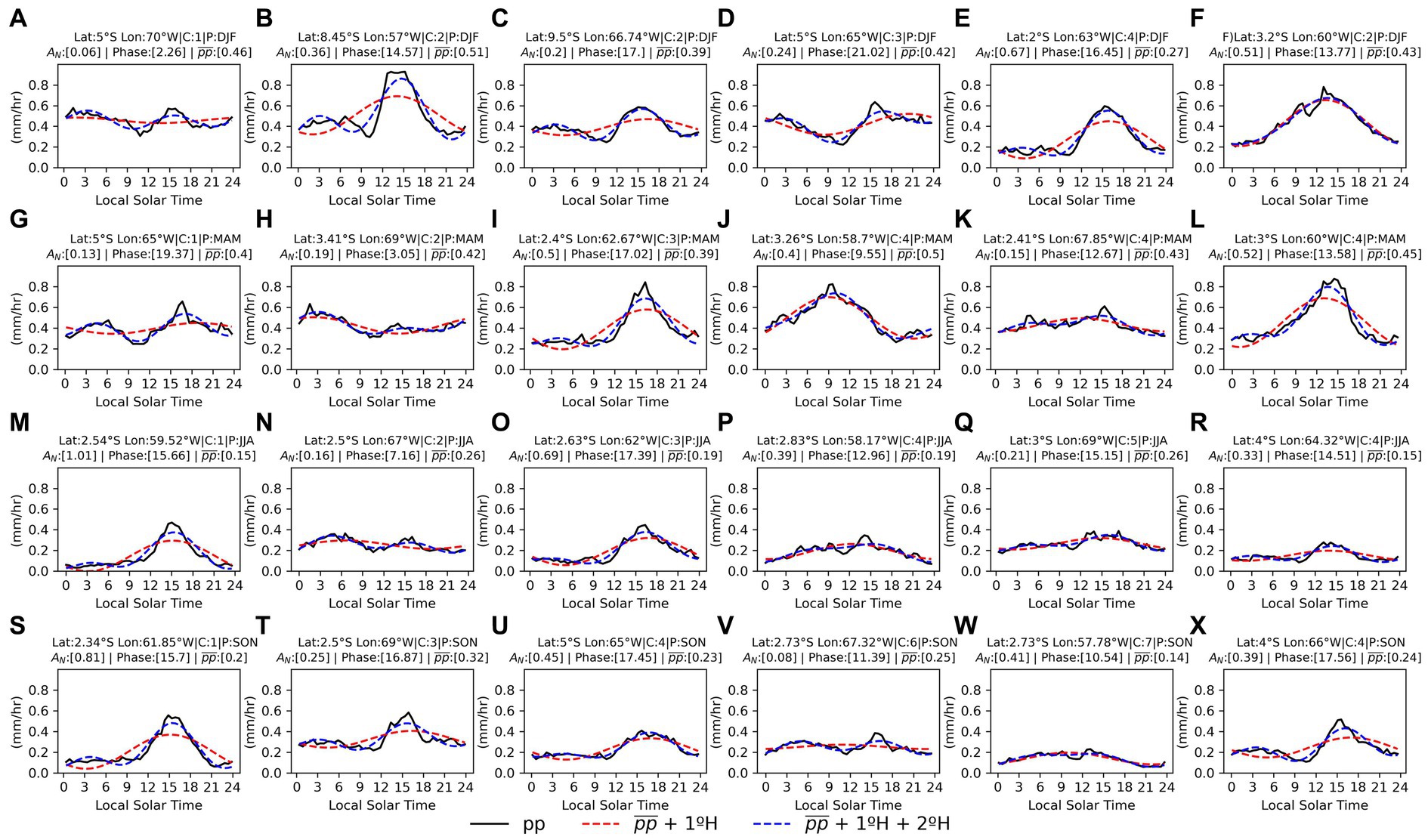
Figure 10. Time series analysis of different types of clusters in the center sector (C) of the Amazon basin. The panels in the first row correspond to the DJF period (A-F), the second row corresponds to the MAM period (G–L), the third row corresponds to the JJA period (M–R), and the last row corresponds to the SON period (S–X). The letter “C” in each panel indicates the label of the cluster in a given period of the year. The black curve represents the mean diurnal cycle of precipitation rate (mm/h). The red curve represents the 24-h oscillation plus the mean precipitation rate. The blue contour represents the mean precipitation rate plus the 24-h and 12-h oscillations.

The DJF period (first row, Figures 10A–F) the central region presents 4 types of clusters: cluster-1, cluster-2, cluster-3 and cluster-4. Clusters’ precipitation rates range from 0.27–0.51 mm/h. The clusters have a bimodal diurnal distribution, with the exception of cluster-4, which has a unimodal distribution. As can be seen in the first row of Figure 10, the clusters differ both in the precipitation rate, the shape of the diurnal cycle distribution and the predominant time of occurrence of the peaks. For example, cluster-1 presents its most intense peak in the dawn (02 LST) and the second lowest intensity peak in the afternoon around 15 LST (Figure 10A). Cluster-2 experiences its largest peak in the afternoon (14–17 LST) and the second peak in the dawn (03–06 LST). Cluster-3 presents a similar behavior to cluster-2 in the time of occurrence of the peaks, but differs in the intensity of the precipitation rates. Finally, cluster-4 presents a unimodal behavior with its peak occurring in the afternoon (16 LST).

For MAM (second row, Figures 10G–L) the central region has 4 clusters (1–4). The precipitation rates of the clusters range from 0.39–0.50 mm/h. Cluster-1 and cluster-2 present a bimodal diurnal distribution, while cluster-3 presents a unimodal diurnal distribution. However, cluster-4 presents a unimodal behavior close to the Amazonas River and the city of Manaus, and as it gets further away from the river its behavior is bimodal. In this period, cluster-1 has its highest intensity peak around 16 LST, and the lowest intensity peak occurs in the early morning (04–06 LST). For cluster-2 the predominant times of its peaks are in the early morning (01–03 LST, peak of highest intensity) and in the afternoon (14–15 LST, peak of lowest intensity). Cluster-3 presents a single predominant time of occurrence of its maximum precipitation rate in the afternoon (16 LST). The bimodal cluster-4 presents its peaks in the morning (09 LST, higher intensity) and in the evening (21 LST, lower intensity), and in the unimodal case its peak occurs in the afternoon (13–16 LST).

In the JJA period (third row, Figures 10M–R) there are 5 different types of diurnal cycle behaviors (clusters 1–5). In this period the precipitation rates range from 0.15–0.26 mm/h. Cluster-1 and cluster-3 present a unimodal diurnal distribution with their peaks occurring 15 LST and 16 LST, respectively. Cluster-2, cluster-4 and cluster-5 present a bimodal/uniform diurnal distribution. Cluster-2 has a peak of highest intensity between dawn and morning (04–07 LST) and the lowest intensity occurring in the afternoon (15–16 LST). Cluster-4 has a clear peak in the afternoon (15 LST) and weak peaks in the early morning (04–05 LST) and morning (07–09 LST). Cluster-5 with a uniform diurnal distribution has a weak peak in the afternoon (13–15 LST).

For SON, the central region of the CA presents 5 types of clusters (1, 3, 4, 6 and 7, see last row of Figures 10S–X). The precipitation rate of the clusters ranges from 0.14–0.32 mm/h. The clusters have a bimodal/uniform diurnal distribution, except for cluster-1 which exhibits unimodal behavior, with its peak happening predominantly between 14 and 16 LST. Cluster-3 and cluster-4 have higher intensity peaks occurring in the afternoon (15–16 LST) and lower peaks occurring in the early morning (03–05 LST). Cluster-6 and cluster-7 have an almost uniform distribution with lower intensity peaks in the early morning (03–06 LST) and a slightly more pronounced peak in the afternoon (14–16 LST).

4 Summary and conclusion

Our results evaluated the heterogeneity of the diurnal cycle of precipitation in the Amazon Basin (AB) identified by comparable past studies in different regions of the basin (Angelis et al., 2004; Tanaka et al., 2014, Nunes et al., 2016; Saraiva et al., 2016; Ruiz-Hernández et al., 2021 and others). This heterogeneity was agglomerated into groups based on precipitation rate, diurnal distribution shape and phase, varying in space–time, coinciding with the circulation large-scale and mechanisms responsible for the onset of the convection. This is the classical behavior of tropical precipitation where surface heterogeneity and diurnal thermal contrast modulate both local-to-regional scale diurnal circulations and the mechanisms responsible for convection initiation (Junquas et al., 2018; Ruiz-Hernández et al., 2021). We analyzed the spatio-temporal variability of the diurnal cycle of precipitation in the AB and performed a regionalization of the different diurnal cycles through cluster analysis. The precipitation rate estimation product IMERG V06B Final Run PrecipitationCal was used with a spatial resolution of 0.1° × 0.1° and temporal resolution of 0.5 h for the period 2001–2020. The harmonic parameters: hourly mean precipitation rate, normalized amplitude and phase, proved to be useful metrics for the quantification and regionalization of the diurnal cycle (Covey et al., 2016).

The precipitation rate and normalized amplitude of the first harmonic allowed us to identify a significant spatio-temporal variability of the diurnal cycle of precipitation. The temporal variability of the heterogeneity of the diurnal cycle of precipitation showed a clear seasonality linked to the seasonal activity of the Mesoscale Convective Systems (MCSs) responsible for organizing precipitation in the AB (Nesbitt et al., 2006). Thus, the temporal variability shows a seasonal shift in precipitation rates generated by MCSs (precipitation rate > 0.254 mm/h, Rehbein et al., 2019, which is associated with large-scale mechanisms linked to the SAMS’ (South American Monsoon System) life cycle (Vera et al., 2006), i.e., related to the regional circulation (Supplementary Figures S1, S2) and local-regional scale processes that induce precipitation. The normalized amplitude associated with a bimodal/uniform diurnal cycle distribution also showed a seasonal shift and linked to the geometric centers of the MCSs observed in past studies (Rehbein, 2021; Rehbein et al., 2017). From the precipitation rate and normalized amplitude it is clear that it is the MCSs that are the main systems distributing precipitation throughout of the AB (Nesbitt et al., 2006) and most of this precipitation is concentrated between the months of December–May (Rao et al., 1996).

Spatial variability of the diurnal cycle, even among nearby clusters, is strongly determined by local factors, thus modulating the intensity, shape of the diurnal distribution and timing of the precipitation peak. For example, in each period, we observed a strong spatial gradient in precipitation rates, highlighting the western region of the AB (Figure 4) associated with the strong topographic gradient of the Andes Mountains. Therefore, in the western part of the AB flanked by the Andes Mountains, it is clearly evident that the topography factor and its windward and leeward configurations determine a strong heterogeneity of the diurnal cycle (Figures 4–6). The phase of the first harmonic allowed us to identify the predominant time of occurrence of the precipitation rate peaks, the displacement of the systems in their different stages in the AB and the link of the diurnal cycle with local factors (rivers, topography, type of surface). The afternoon precipitation peaks (Figure 6) on the Andean ridges would be related to local convection and valley-mountain breezes (anabatic winds) induced by differential heating between mountain slopes and Andean valleys. On the eastern slopes of the Andes, at the foot of the mountains and toward the valleys, precipitation peaks are observed occurring from the night to early morning hours, indicating an eastward shift of the AB of the SCMs. These systems are also called Andes Occurring Systems (AOS, Bendix et al., 2006) and are characterized by the formation of rain bands with eastward and southward displacement in the AB. The AOS are formed by the interaction between the local scale katabatic winds flowing from the Andes toward the Amazon rainforest and interacting with the humid and warm air coming from the Amazon and with the large-scale flow channeled by the mechanical action of the topographic barrier of the Andes. In the northern and northeastern part of the AB, the proximity to the sea and the elevation of the terrain are the main factors that induce a heterogeneous behavior of the diurnal cycle. The main systems acting in these regions are the squall lines originated by the sea breeze front (Burleyson et al., 2016) produced by a thermal differential between the sea and the continent. Thus, regions close to the coast experience peaks in the late afternoon and the further away from the coast the peaks occur between night and early morning. As these systems move toward the interior of the AB, they lose intensity and dissipate, serving as a source of moisture for the atmosphere and this moisture is recycled to form new systems that will continue to move toward the center of the AB. Other factors such as the presence of large Amazonian rivers and their seasonal flooding cycle, urban cities and their heat island effect are determinants in the diurnal distribution and predominant times of occurrence of the peaks. Also, it has been noted in past studies that the seasonality of forest fires and their aerosol contributions to the atmosphere impact the intensity of the diurnal cycle, generating more intense convective activity with lightning incidence (Albrecht et al., 2011; Andreae et al., 2004; Gonçalves et al., 2015; Martins et al., 2009).

Using cluster analysis, we identified for the DJF, MAM and JJA periods, for the first time, six (seven for the SON period) different types of diurnal cycle behaviors as a function of their precipitation rate, distribution shape and phase. Through the spatial distribution of the clusters, we identify that their configuration varies seasonally, and it may be the SAMS and large-scale physical mechanisms that configure their spatial distribution. However, we observe that local factors modulate the intensity, the shape of the diurnal cycle distribution, and the time of day of maximum occurrence. The findings of this work complement previous studies in different regions within of the AB that analyzed the diurnal cycle over different surfaces, but from a global view, showing that the diurnal cycle of precipitation is heterogeneous.

A detailed understanding of the diurnal cycle of precipitation in the AB requires high-resolution numerical modeling studies of the atmosphere to investigate how certain processes control the diurnal cycle in specific clusters. It is of interest to know the role that certain meteorological phenomena would have on the behavior of the diurnal cycle, e.g., LLJA (Anselmo et al., 2020) and LLJSA (Marengo et al., 2004) episodes. The application of artificial intelligence algorithms to understand the degree of contribution of different drivers acting on a cluster could bring light to improve our picture of the diurnal cycle in the AB and thus be able to improve the representation of this mode of fine-scale variability of the next generation of numerical weather and climate models.

The knowledge gained in this study could help to improve the representation of the diurnal cycle of precipitation in state-of-the-art weather and climate models, which to date fail to adequately represent its intensity and phase (e.g., Dai, 2006; Da Rocha et al., 2009; Dirmeyer et al., 2012; Watters et al., 2021). In addition, it lays the groundwork for future research on the role of local factors and different triggers linked to the heterogeneous diurnal cycle of precipitation experienced by the AB. For example, understanding how the presence of a river and the seasonal flooding it experiences can affect the thermally induced local circulations and the formation of a certain behavior of the diurnal cycle of precipitation.

Data availability statement

The datasets presented in this study can be found in online repositories. The names of the repository/repositories and accession number(s) can be found in the article/Supplementary material.

Author contributions

RR-N: Conceptualization, Data curation, Formal analysis, Funding acquisition, Investigation, Methodology, Project administration, Resources, Software, Validation, Visualization, Writing – original draft, Writing – review & editing. MS: Conceptualization, Formal analysis, Funding acquisition, Methodology, Project administration, Resources, Supervision, Visualization, Writing – review & editing.

Funding

The author(s) declare that financial support was received for the research, authorship, and/or publication of this article. The research has been funded by Fundação de Amparo à Pesquisa do Estado de São Paulo (FAPESP) Grant 2017/17047-0 and by graduate student scholarship by Conselho Nacional de Desenvolvimento Científico e Tecnológico (CNPq) grant 131010/2020-4.

Conflict of interest

The authors declare that the research was conducted in the absence of any commercial or financial relationships that could be construed as a potential conflict of interest.

Publisher’s note

All claims expressed in this article are solely those of the authors and do not necessarily represent those of their affiliated organizations, or those of the publisher, the editors and the reviewers. Any product that may be evaluated in this article, or claim that may be made by its manufacturer, is not guaranteed or endorsed by the publisher.

Supplementary material

The Supplementary material for this article can be found online at: https://www.frontiersin.org/articles/10.3389/fclim.2024.1370097/full#supplementary-material

References

Albrecht, R. I., Rodríguez, C. A. M., and Silva Dias, M. A. F. da. (2011). Electrification of precipitating systems over the Amazon: physical processes of thunderstorm development. J. Geophys. Res. Atmos. 116. doi: 10.1029/2010JD014756

Crossref Full Text | Google Scholar

Alcântara, C. R., Dias, M. A. S., Souza, E. P., and Cohen, J. C. (2011). Verification of the role of the low level jets in Amazon squall lines. Atmos. Res. 100:36. doi: 10.1016/j.atmosres.2010.12.023

Crossref Full Text | Google Scholar

ANA. (2014). Região hidrográfica da Amazônia. Available at: http://www2.ana.gov.br/Paginas/portais/bacias/amazonica.aspx (Accessed March 29, 2021)

Google Scholar

ANA. (2019). Expedição quer provar que o rio Amazonas é maior que o Nilo. Available at: http://www.ana.gov.br/noticias-antigas/expediassapso-quer-provar-que-o-rio-amazonas-a-c.2019-03-14.9802971096 (Accessed March 29, 2021)

Google Scholar

Andreae, M. O., Rosenfeld, D., Artaxo, P., Costa, A., Frank, G., Longo, K., et al. (2004). Smoking rain clouds over the Amazon. Science 303:1337. doi: 10.1126/science.1092779

PubMed Abstract | Crossref Full Text | Google Scholar

Angelis, C. F., McGregor, G. R., and Kidd, C. (2004). Diurnal cycle of rainfall over the Brazilian Amazon. Clim. Res. 26:139. doi: 10.3354/cr026139

PubMed Abstract | Crossref Full Text | Google Scholar

Anselmo, E. M., Machado, L. A., Schumacher, C., and Kiladis, G. N. (2021). Amazonian mesoscale convective systems: life cycle and propagation characteristics. Int. J. Climatol. 41:3968. doi: 10.1002/joc.7053

Crossref Full Text | Google Scholar

Anselmo, E. M., Schumacher, C., and Machado, L. A. (2020). The Amazonian low-level jet and its connection to convective cloud propagation and evolution. Mon. Weather Rev. 148:4083. doi: 10.1175/MWR-D-19-0414.1

Crossref Full Text | Google Scholar

Arraut, J. M., Nobre, C., Barbosa, H. M., Obregon, G., and Marengo, J. (2012). Aerial rivers and lakes: looking at large-scale moisture transport and its relation to Amazonia and to subtropical rainfall in South America. J. Clim. 25:543. doi: 10.1175/2011JCLI4189.1

Crossref Full Text | Google Scholar

Bendix, J., Rollenbeck, R., Göttlicher, D., and Cermák, J. (2006). Cloud occurrence and cloud properties in Ecuador. Clim. Res. 30, 133–147. doi: 10.3354/cr030133

Crossref Full Text | Google Scholar

Biasutti, M., and Yuter, S. E. (2013). Observed frequency and intensity of tropical precipitation from instantaneous estimates. J. Geophys. Res. Atmos. 118:9534. doi: 10.1002/jgrd.50694

Crossref Full Text | Google Scholar

Burleyson, C. D., Feng, Z., Hagos, S. M., Fast, J., Machado, L. A., and Martin, S. T. (2016). Spatial variability of the background diurnal cycle of deep convection around the GoAmazon2014/5 field campaign sites. J. Appl. Meteorol. Climatol. 55:1579. doi: 10.1175/JAMC-D-15-0229.1

Crossref Full Text | Google Scholar

Callède, J., Cochonneau, G., Alves, F., Guyot, J.-L., Guimarães, V., and De Oliveira, E. (2010). Les apports en eau de l’Amazone à l’Océan Atlantique. J. Water Sci. 23:247. doi: 10.7202/044688ar

Crossref Full Text | Google Scholar

Callède, J., Guyot, J.-L., Ronchail, J., and Oliveira, E. (2004). Evolution du débit de l’Amazone à Óbidos de 1903 à 1999. Hydrol. Sci. J. 49:85. doi: 10.1623/hysj.49.1.85.53992

Crossref Full Text | Google Scholar

Carvalho, L. M. V., Jones, C., and Liebmann, B. (2004). The South Atlantic convergence zone: intensity, form, persistence, and relationships with Intraseasonal to interannual activity and extreme rainfall. J. Clim. 17, 88–108. doi: 10.1175/1520-0442(2004)017<0088:TSACZI>2.0.CO;2

Crossref Full Text | Google Scholar

Carvalho, L. M., Jones, C., and Silva, D. M. (2002). Intraseasonal large-scale circulations and mesoscale convective activity in tropical South America during the TRMM-LBA campaign. J. Geophys. Res. Atmos. 107, 1–9. doi: 10.1029/2001jd000745

Crossref Full Text | Google Scholar

Carvalho, L. M., Jones, C., Silva, A. E., Liebmann, B., and Silva, D. P. (2011). The south American monsoon system and the 1970s climate transition. Int. J. Climatol. 31:1248. doi: 10.1002/joc.2147

Crossref Full Text | Google Scholar

Chavez, S. P., and Takahashi, K. (2017). Orographic rainfall hot spots in the Andes-Amazon transition according to the TRMM precipitation radar and in situ data. J. Geophys. Res. Atmos. 122:5870. doi: 10.1002/2016JD026282

Crossref Full Text | Google Scholar

Cohen, J. C. P., Fitzjarrald, D. R., D’Oliveira, F. A. F., Saraiva, I., Barbosa, I. R. D. S., Gandu, A. W., et al. (2014). Radar-observed spatial and temporal rainfall variability near the Tapajós-Amazon confluence. Rev. Brasil. Meteorol. 29:23. doi: 10.1590/0102-778620130058

Crossref Full Text | Google Scholar

Cohen, J. C., Silva Dias, M. A., and Nobre, C. A. (1995). Environmental conditions associated with Amazonian squall lines: a case study. Mon. Weather Rev. 123:3163. doi: 10.1175/1520-0493(1995)123<3163:ECAWAS>2.0.CO;2

Crossref Full Text | Google Scholar

Covey, C., Gleckler, P. J., Doutriaux, C., Williams, D. N., Dai, A., Fasullo, J., et al. (2016). Metrics for the diurnal cycle of precipitation: toward routine benchmarks for climate models. J. Clim. 29:4461. doi: 10.1175/JCLI-D-15-0664.1

Crossref Full Text | Google Scholar

Cutrim, E. M., Martin, D. W., Butzow, D. G., Silva, I. M., and Yulaeva, E. (2000). Pilot analysis of hourly rainfall in central and eastern Amazonia. J. Clim. 13:1326. doi: 10.1175/1520-0442(2000)013<1326:PAOHRI>2.0.CO;2

Crossref Full Text | Google Scholar

Da Rocha, R. P., Morales, C. A., Cuadra, S. V., and Ambrizzi, T. (2009). Precipitation diurnal cycle and summer climatology assessment over South America: an evaluation of regional climate model version 3 simulations. J. Geophys. Res. Atmos. 114:D10108. doi: 10.1029/2008JD010212

Crossref Full Text | Google Scholar

Dai, A. (2006). Precipitation characteristics in eighteen coupled climate models. J. Clim. 19:4605. doi: 10.1175/JCLI3884.1

Crossref Full Text | Google Scholar

Dirmeyer, P. A., Cash, B. A., Kinter, J. L., Jung, T., Marx, L., Satoh, M., et al. (2012). Simulating the diurnal cycle of rainfall in global climate models: resolution versus parameterization. Clim. Dyn. 39:399. doi: 10.1007/s00382-011-1127-9

Crossref Full Text | Google Scholar

dos Santos, M. J., Silva, D. M., and Freitas, E. D. (2014). Influence of local circulations on wind, moisture, and precipitation close to Manaus City, Amazon Region, Brazil. J. Geophysic. Res. 119:13. doi: 10.1002/2014JD021969

Crossref Full Text | Google Scholar

Easterling, D. R., and Robinson, P. J. (1985). The diurnal variation of thunderstorm activity in the United States. J. Appl. Meteorol. Climatol. 24:1048.

Google Scholar

Espinoza, J. C., Chavez, S., Ronchail, J., Junquas, C., Takahashi, K., and Lavado, W. (2015). Rainfall hotspots over the southern tropical Andes: spatial distribution, rainfall intensity, and relations with large-scale atmospheric circulation. Water Resour. Res. 51:3459. doi: 10.1002/2014WR016273

Crossref Full Text | Google Scholar

Espinoza, J. C., Garreaud, R., Poveda, G., Arias, P. A., Molina-Carpio, J., Masiokas, M., et al. (2020). Hydroclimate of the Andes part I: main climatic features. Front. Earth Sci. 8:65. doi: 10.3389/feart.2020.00064

Crossref Full Text | Google Scholar

Espinoza, J. C., Lengaigne, M., Ronchail, J., and Janicot, S. (2012). Large-scale circulation patterns and related rainfall in the Amazon Basin: a neuronal networks approach. Clim. Dyn. 38:121. doi: 10.1007/s00382-011-1010-8

Crossref Full Text | Google Scholar

Espinoza, J. C., Ronchail, J., Guyot, J. L., Cochonneau, G., Naziano, F., Lavado, W., et al. (2009). Spatio-temporal rainfall variability in the Amazon basin countries (Brazil, Peru, Bolivia, Colombia, and Ecuador). Int. J. Climatol. 29:1574. doi: 10.1002/joc.1791

Crossref Full Text | Google Scholar

Espinoza, J. C., Ronchail, J., Lengaigne, M., Quispe, N., Silva, Y., Bettolli, M. L., et al. (2013). Revisiting wintertime cold air intrusions at the east of the Andes: propagating features from subtropical Argentina to Peruvian Amazon and relationship with large-scale circulation patterns. Clim. Dyn. 41:1983. doi: 10.1007/s00382-012-1639-y

Crossref Full Text | Google Scholar

Figueroa, S. N., and Nobre, C. A. (1990). Precipitation distribution over central and western tropical South America. Climanálise 5:36.

Google Scholar

Fisch, G., Marengo, J. A., and Nobre, C. A. (1998). Uma revisão geral sobre o clima da Amazônia. Acta amazônica 28:101. doi: 10.1590/1809-43921998282126

Crossref Full Text | Google Scholar

Gonçalves, W., Machado, L., and Kirstetter, P.-E. (2015). Influence of biomass aerosol on precipitation over the Central Amazon: an observational study. Atmos. Chem. Phys. 15:6789. doi: 10.5194/acp-15-6789-2015

Crossref Full Text | Google Scholar

Hayden, L. J. M., Tan, J., Bolvin, D. T., and Huffman, G. J. (2023). Variations in the diurnal cycle of precipitation and its changes with distance from shore over two contrasting regions as observed by IMERG, ERA5, and Spaceborne Ku radar. J. Hydrometeorol. 24, 675–689. doi: 10.1175/JHM-D-22-0154.1

Crossref Full Text | Google Scholar

Hersbach, H., Bell, B., Berrisford, P., Hirahara, S., Horányi, A., Muñoz-Sabater, J., et al. (2020). The ERA5 global reanalysis. Q. J. R. Meteorol. Soc. 146:1999. doi: 10.1002/qj.3803

PubMed Abstract | Crossref Full Text | Google Scholar

Huffman, G., Braithwaite, D., Hsu, K., Joyce, R., Kidd, C., Nelkin, E., et al. (2020). Integrated Multi-satellite Retrievals for the Global Precipitation Measurement (GPM) Mission (IMERG). In: V. Levizzani, C. Kidd, D. B. Kirschbaum, C. D. Kummerow, K. Nakamura, and F. J. Turk (eds) Satellite Precipitation Measurement. Advances in Global Change Research, vol 67. Springer: Cham. doi: 10.1007/978-3-030-24568-9_19

Crossref Full Text | Google Scholar

Huffman, G. J., Stocker, E. F., Bolvin, D. T., Nelkin, E. J., and Tan, J., (2019) GPM IMERG final precipitation L3 half hourly 0.1 degree x 0.1 degree V06, greenbelt, MD, Goddard earth sciences data and information services Center (GES DISC). (Accessed November 1, 2021).

Google Scholar

Ilbay-Yupa, M., Lavado-Casimiro, W., Rau, P., Zubieta, R., and Castillón, F. (2021). Updating regionalization of precipitation in Ecuador. Theor. Appl. Climatol. 143:1513. doi: 10.1007/s00704-020-03476-x

PubMed Abstract | Crossref Full Text | Google Scholar

Janowiak, J. E., Kousky, V. E., and Joyce, R. J. (2005). Diurnal cycle of precipitation determined from the CMORPH high spatial and temporal resolution global precipitation analyses. J. Geophys. Res. Atmos. 110:D23105. doi: 10.1029/2005JD006156

Crossref Full Text | Google Scholar

Junquas, C., Takahashi, K., Condom, T., Espinoza, J.-C., Chávez, S., Sicart, J.-E., et al. (2018). Understanding the influence of orography on the precipitation diurnal cycle and the associated atmospheric processes in the Central Andes. Clim. Dyn. 50:3995. doi: 10.1007/s00382-017-3858-8

Crossref Full Text | Google Scholar

López, K. L. C. (2020). Interannual variability of tropical Atlantic and its influence on extreme precipitation events: focus on the Amazon Basin. Tese de Doutorado: Universidade de São Paulo.

Google Scholar

Lorenz, E. N. (1956). Empirical orthogonal functions and statistical weather prediction. Cambridge: Massachusetts Institute of Technology, Department of Meteorology.

Google Scholar

Marengo, J., and Nobre, C. A. (2009). Clima da região Amazônica. Tempo Clima Brasil 1:198.

Google Scholar

Marengo, J. A., Soares, W. R., Saulo, C., and Nicolini, M. (2004). Climatology of the low-level jet east of the Andes as derived from the NCEP–NCAR reanalyses: characteristics and temporal variability. J. Clim. 17:2261. doi: 10.1175/1520-0442(2004)017<2261:COTLJE>2.0.CO;2

Crossref Full Text | Google Scholar

Martins, J., Silva Dias, M. A. F. D., and Gonçalves, F. L. T. (2009). Impact of biomass burning aerosols on precipitation in the Amazon: a modeling case study. J. Geophys. Res. Atmos. 114:D02207. doi: 10.1029/2007JD009587

Crossref Full Text | Google Scholar

Mayta, V. C., Silva, N. P., Ambrizzi, T., Dias, P. L. S., and Espinoza, J. C. (2020). Assessing the skill of all-season diverse madden–Julian oscillation indices for the intraseasonal Amazon precipitation. Clim. Dyn. 54:3729. doi: 10.1007/s00382-020-05202-9

Crossref Full Text | Google Scholar

Molinier, M., Guyot, J-L, Oliveira, E., and Guimaraes, V. (1996). Les régimes hydrologiques de l’Amazone et de ses affluents. In: P. Chevallier and B. Pouyaud (eds). L’hydrologie tropicale: géosciences et outil pour le développement: mélanges à la mémoire de Jean Rodier. Wallingford: AISH, p. 209–222. (Publication - AISH; 238). Journées Hydrologiques de l’ORSTOM: Conférence de Paris, 11., Paris (FRA), 1995/05/02-04.

Google Scholar

Nesbitt, S. W., Cifelli, R., and Rutledge, S. A. (2006). Storm morphology and rainfall characteristics of TRMM precipitation features. Mon. Weather Rev. 134:2702. doi: 10.1175/MWR3200.1

Crossref Full Text | Google Scholar

Nunes, A. M., Silva Dias, M. A., Anselmo, E. M., and Morales, C. A. (2016). Severe convection features in the Amazon Basin: a TRMM-based 15-year evaluation. Front. Earth Sci. 4:37. doi: 10.3389/feart.2016.00037

Crossref Full Text | Google Scholar

Paccini, L., and Stevens, B. (2023). Assessing precipitation over the Amazon basin as simulated by a storm-resolving model. J. Geophys. Res. Atmos. 128:e2022JD037436. doi: 10.1029/2022JD037436

Crossref Full Text | Google Scholar

Paiva, R. C. D., Buarque, D. C., Clarke, R. T., Collischonn, W., and Allasia, D. G. (2011). Reduced precipitation over large water bodies in the Brazilian Amazon shown from TRMM data. Geophys. Res. Lett. 38:L04406. doi: 10.1029/2010GL045277

Crossref Full Text | Google Scholar

Poveda, G., Mesa, O. J., Salazar, L. F., Arias, P. A., Moreno, H. A., Vieira, S. C., et al. (2005). The diurnal cycle of precipitation in the tropical Andes of Colombia. Mon. Weather Rev. 133:228. doi: 10.1175/MWR-2853.1

Crossref Full Text | Google Scholar

Rao, V. B., Cavalcanti, I. F., and Hada, K. (1996). Annual variation of rainfall over Brazil and water vapor characteristics over South America. J. Geophys. Res. Atmos. 101:26539. doi: 10.1029/96JD01936

Crossref Full Text | Google Scholar

Rehbein, A. (2021). Sistemas convectivos de mesoescala na bacia Amazônica: clima presente e projeções futuras em cenários de mudanças climáticas. Tese de Doutorado: Universidade de São Paulo.

Google Scholar

Rehbein, A., and Ambrizzi, T. (2023). Mesoscale convective systems over the Amazon basin in a changing climate under global warming. Clim. Dyn. 61, 1815–1827. doi: 10.1007/s00382-022-06657-8

Crossref Full Text | Google Scholar

Rehbein, A., Ambrizzi, T., and Mechoso, C. R. (2017). Mesoscale convective systems over the Amazon basin. Part I: climatological aspects. Int. J. Climatol. 38, 215–229. doi: 10.1002/joc.5171

Crossref Full Text | Google Scholar

Rehbein, A., Ambrizzi, T., Mechoso, C. R., Ibarra-Espinosa, S., and Myers, T. A. (2019). Mesoscale convective systems over the Amazon basin: the GoAmazon2014/5 program. Int. J. Climatol. 39, 5599–5618. doi: 10.1002/joc.6173

Crossref Full Text | Google Scholar

Rousseeuw, P. J. (1987). Silhouettes: a graphical aid to the interpretation and validation of cluster analysis. J. Comput. Appl. Math. 20:53. doi: 10.1016/0377-0427(87)90125-7

Crossref Full Text | Google Scholar

Ruiz-Hernández, J.-C., Condom, T., Ribstein, P., Le Moine, N., Espinoza, J.-C., Junquas, C., Villacı́s, M., Vera, A., Muñoz, T., Maisincho, L., et al. Spatial variability of diurnal to seasonal cycles of precipitation from a high-altitude equatorial Andean valley to the Amazon Basin, journal of hydrology: Reg. Stud. (2021). vol. 38:100924. doi: 10.1016/j.ejrh.2021.100924

Crossref Full Text | Google Scholar

Santos, M. J., Medvigy, D., Silva Dias, M. A., Freitas, E. D., and Kim, H. (2019). Seasonal flooding causes intensification of the river breeze in the Central Amazon. J. Geophys. Res. Atmos. 124:5178. doi: 10.1029/2018JD029439

Crossref Full Text | Google Scholar

Sapucci, C., Mayta, V., and Silva, D. P. (2022). Evaluation of diverse-based precipitation data over the Amazon region. Theor. Appl. Climatol. 149, 1167–1193. doi: 10.1007/s00704-022-04087-4

Crossref Full Text | Google Scholar

Saraiva, I., Dias, M. A. F. S., Morales, C. A. R., and Saraiva, J. M. B. (2016). Regional variability of rain clouds in the Amazon Basin as seen by a network of weather radars. J. Appl. Meteorol. Climatol. 55:2657. doi: 10.1175/JAMC-D-15-0183.1

Crossref Full Text | Google Scholar

Satyamurty, P., Nobre, C. A., and Silva, D. P. (1998). Meteorology of the southern hemisphere : Springer, Boston: American Meteorological Society. 119–139.

Google Scholar

Silva, D. M., Silva, D. P., Longo, M., Fitzjarrald, D. R., and Denning, A. S. (2004). River breeze circulation in eastern Amazonia: observations and modelling results. Theor. Appl. Climatol. 78, 111–121. doi: 10.1007/s00704-004-0047-6

Crossref Full Text | Google Scholar

Tan, J., Huffman, G. J., Bolvin, D. T., and Nelkin, E. J. (2019). Diurnal cycle of IMERG V06 precipitation. Geophys. Res. Lett. 46:13584. doi: 10.1029/2019GL085395

Crossref Full Text | Google Scholar

Tanaka, L. M. D. S., Satyamurty, P., and Machado, L. A. T. (2014). Diurnal variation of precipitation in Central Amazon Basin. Int. J. Climatol. 34:3574. doi: 10.1002/joc.3929

Crossref Full Text | Google Scholar

Van Der Maaten, L., Postma, E., and Van den Herik, J. (2009). Dimensionality reduction: a comparative. J. Mach. Learn. Res. 10:13.

Google Scholar

Vera, C., Higgins, W., Amador, J., Ambrizzi, T., Garreaud, R., Gochis, D., et al. (2006). Toward a unified view of the American monsoon systems. J. Clim. 19:4977. doi: 10.1175/JCLI3896.1

Crossref Full Text | Google Scholar

Watters, D., and Battaglia, A. (2019). The summertime diurnal cycle of precipitation derived from IMERG. Remote Sens. 11:1781. doi: 10.3390/rs11151781

Crossref Full Text | Google Scholar

Watters, D., Battaglia, A., and Allan, R. P. (2021). The diurnal cycle of precipitation according to multiple decades of global satellite observations, three CMIP6 models, and the ECMWF reanalysis. J. Clim. 34:5063. doi: 10.1175/JCLI-D-20-0966.1

Crossref Full Text | Google Scholar

Webler, A. D., Aguiar, R. G., and Aguiar, L. J. (2007). Características da precipitação em área de floresta primária e área de pastagem no Estado de Rondônia, Ciência e. Natura, 55–58. doi: 10.5902/2179460X9755

Crossref Full Text | Google Scholar

Wilks, D. S. (2011). Statistical methods in the atmospheric sciences, 3rd Edn. vol. 100. Oxford: Academic press.

Google Scholar

Yang, G.-Y., and Slingo, J. (2001). The diurnal cycle in the tropics. Mon. Weather Rev. 129:784. doi: 10.1175/1520-0493(2001)129<0784:TDCITT>2.0.CO;2

PubMed Abstract | Crossref Full Text | Google Scholar

Zängl, G., Reinert, D., Rípodas, P., and Baldauf, M. (2015). The ICON (ICOsahedral non-hydrostatic) modelling framework of DWD and MPI-M: description of the non-hydrostatic dynamical core. Meteorol. Soc. 141, 563–579. doi: 10.1002/qj.2378

Crossref Full Text | Google Scholar