On the uncertainty of long-period return values of extreme daily precipitation

Methods for calculating return values of extreme precipitation and their uncertainty are compared using daily precipitation rates over the Western U.S. and Southwestern Canada from a large ensemble of climate model simulations. The roles of return-value estimation procedures and sample size in uncertainty are evaluated for various return periods. We compare two different generalized extreme value (GEV) parameter estimation techniques, namely L-moments and maximum likelihood (MLE), as well as empirical techniques. Even for very large datasets, confidence intervals calculated using GEV techniques are narrower than those calculated using empirical methods. Furthermore, the more efficient L-moments parameter estimation techniques result in narrower confidence intervals than MLE parameter estimation techniques at small sample sizes, but similar best estimates. It should be noted that we do not claim that either parameter fitting technique is better calibrated than the other to estimate long period return values. While a non-stationary MLE methodology is readily available to estimate GEV parameters, it is not for the L-moments method. Comparison of uncertainty quantification methods are found to yield significantly different estimates for small sample sizes but converge to similar results as sample size increases. Finally, practical recommendations about the length and size of climate model ensemble simulations and the choice of statistical methods to robustly estimate long period return values of extreme daily precipitation statistics and quantify their uncertainty.

1 Introduction

There are numerous sources of uncertainty in both observed and simulated climate statistics. The finite length of climate data records is a source of uncertainty due to the intrinsically chaotic nature of the Earth’s climate system. Although a significant source of uncertainty in describing the mean climate, this sample size uncertainty is exacerbated for extreme values, as the tail of a distribution is only a subset of the already limited parent sample. While ensemble climate model simulations, especially the newly available Large Ensemble Simulations (LENS), that provide statistical replicates through multiple independent realizations can alleviate the data length shortcomings, this is not possible for the observations. Analysts must be aware of other observational shortcomings such as station relocations, instrumental errors and other data processing errors. Transforming from pointwise weather station data to a regular grid can introduce other errors, especially regarding extreme precipitation (Chen and Knutson, 2008; Gervais et al., 2014; Risser and Wehner, 2020; Wehner et al., 2021). Climate model simulations of the past and future climate contain additional uncertainties from the imperfect nature of the climate model simulations themselves. Indeed, such model structural differences are the largest source of uncertainty in long term climate change projections under a specific emissions scenario or fixed global warming level (Hawkins and Sutton, 2009). Sample size and methodological choices can also limit how extreme the subset of the parent data might be leading to biases in estimation of long period return values due to violation of the assumptions of extreme value theory. Here we use a single climate model to generate a very large extreme value sample to explore the properties of sample size uncertainty, but we neglect uncertainty due to model imperfections and differences.

Extreme value theory provides a rigorous and formal method to both extrapolate and interpolate the properties of the tails of distributions under a suitable set of assumptions (Coles, 2001). A previous study (Wehner, 2010) demonstrated that sample size is an important source of uncertainty in the estimation of 20-year return values of the annual maxima of daily temperatures from publicly available multi-model datasets (i.e., Kharin et al., 2013). However, sample size uncertainty was found to be smaller than the structural uncertainty across different climate models of the same class. While not investigated here, model structural uncertainty is likely larger for extreme precipitation than for extreme temperature due to the variety of moist physics parameterization schemes (Hawkins and Sutton, 2011).

In addition to model structural uncertainty and sample size uncertainty, estimated long-period return values and their uncertainty can vary depending on the statistical methods used. In this study, we investigate statistical uncertainty in simulated long-period return values of daily precipitation for a variety of methodologies and data set sizes. Methods to calculate long-period return values from the tails of samples fall into two broad categories: nonparametric (empirical) and parametric methods. Nonparametric methods, such as calculating a simple percentile threshold, are computationally and conceptually straightforward, and make no assumptions about the nature of the data. In contrast, parametric methods invoke assumptions on the shape of the distribution, and so may introduce bias if the underlying data generation processes do not produce the assumed distribution. A particular class of parametric methods are the often-used generalized extreme value (GEV) methods of fitting a three-parameter distribution to the tail rather than the entire distribution. GEV methods are well supported by statistical theory so long as the dataset satisfy the following assumptions: The data in the tail are independent and identically distributed (“i.i.d.”) and the subsample of the tail of the distribution is sufficiently extreme, technically known as “max-stability” in the statistical literature (Coles, 2001).

We compare the estimation techniques described above for a variety of sample sizes and return periods. Intuitively we expect that the uncertainty from finite sample size is reduced as more data becomes available relative to the length of the return period of interest. For example, estimates of the 1-in-100-year event with 20 years of data should have much larger uncertainty than estimates with 200 years of data. This sample size uncertainty becomes zero in the limit of a complete population of the true climatology regardless of whether a parametric or nonparametric method is used.

In this study, we use simulated daily precipitation in the western U.S. and Southwestern Canada as a test bed for quantifying uncertainty in long-period return values. This is enabled by a very large single-year ensemble simulation made possible through the public computing project, climateprediction.net. While the climate model is not a perfect representation of the earth’s actual climate system, this particular experiment, described below, has two principal advantages over actual observations for this study. First, it generated a very large ensemble of simulations, permitting subsetting to explore sample size effects. Second, all of the realizations of the ensemble simulation are of the same year and hence data from different years are stationary and largely independent from one another, which is advantageous because the GEV distribution assumes that data are stationary, independent, and identically distributed (i.i.d.). Here we use annual-maximum daily precipitation. Annual-maximum daily precipitation data are likely not completely identically-distributed because different precipitation events may result from different underlying weather patterns, especially if extreme precipitation events span different seasons. The western U.S. and Southwestern Canada includes both wet and dry regions with different degrees of variability across time scales with an associated variety of uncertainty properties. Reducing the block size to individual seasons would bring the dataset closer to i.i.d. at the cost of causing it to be further from the asymptotic regime of the tail of the distribution. Furthermore, there is no reason to assume that different storm types within a season would behave in statistically identical manners. Despite these less-than-ideal properties, annual maximum daily precipitation is a commonly used basis for constructing an extreme value sample.

Our intent in this paper is to provide guidance to climate data analysts, not to present any intrinsically new statistical methods. Hence, the primary contributions of this paper are four-fold: to compare uncertainty in estimated precipitation return values between various methods of estimating return values (Section 5); to compare uncertainty in estimated precipitation return values across various sample sizes (Section 6); to compare practical ways of quantifying uncertainty when the sample size is limited (Section 7); and to evaluate whether uncertainty approaches zero at increasing sample size (Section 8). While there are numerous parametric methods for estimating GEV parameters, we focus here on two of the most commonly used fitting methods: maximum likelihood estimation (MLE) and L-moments.

In Section 2 we introduce generalized extreme value theory. In Section 3 we introduce our large model dataset. In Section 4 we describe the climatology of precipitation over the Western US and Southwestern Canada. In Section 5, we compare GEV derived long-period return values to those obtained from a simple non-parametric estimation. In Section 6, by subsampling the entire sample, we explore the return value uncertainty as a function of sample size and return period for the L-moments and MLE parameters estimation methods, finding significant differences between them when sample size is small. In Section 7 using only the MLE fitting procedure, we explore different methods of estimating uncertainty as a function of sample size and return period, again finding significant differences between them when sample size is small. In Section 8 we explore the behavior of uncertainty with increasing sample size. Finally, in the conclusion, we discuss how practitioners can decide what sample size is required for their analyses as well as some guidance to the choice of parameter and uncertainty estimation methods available to them.

2 Materials and methods I: a short description of generalized extreme value theory

The stationary three parameter Generalized Extreme Value (GEV) distribution, G(z),

$G\left(z\right)=\{\begin{array}{cc}\hfill exp\left\{-{\left[1+\xi \left(\frac{z-\mu }{\sigma }\right)\right]}^{-\frac{1}{\xi }}\right\}\hfill & \hfill \xi \ne 0\hfill \\ \hfill exp\left[-exp\left\{-\frac{z-\mu }{\sigma }\right\}\right]\hfill & \hfill \xi =0\hfill \end{array}\text{ (1)}\text{,}$

is the asymptotically-correct function describing the probability distribution function of block maxima where z satisfies $1+\frac{\xi \left(z-\mu \right)}{\sigma }>0$ (Coles, 2001). In our usage of Equation (1), z represents the annual maximum daily precipitation and μ, σ, and ξ are the location, scale, and shape parameters to be estimated. Truly rare precipitation events can be described by considering behavior of the upper tail of the GEV distribution function. The GEV distribution is fitted to “block” maxima (in this case, annual maxima) and inverted to provide estimates of long-period return values across a range of sample sizes and return periods. We note that a transformation to a peaks-over-thresholds methodology and associated Generalized Pareto Distribution can be made (Embrechts et al., 1997; Coles, 2001) but we expect that our conclusions would be similar. As we will see below, simulated precipitation often exhibits a “heavy” tail (ξ > 0). In our stationary example here, the return value, z_T, is that value of the daily precipitation that is exceeded, on average, once every T years over a long period of time. Alternatively, given our assumptions, there is a 1/T chance of any daily average exceeding z_T in a given year (where T is in years). Formally, this is defined as

$\begin{array}{ll}G\left(z_T\right)=1-\frac{T_0}{T}\text{,}& (2)\end{array}$

where T₀ is a characteristic time whose value is 1 year. Solving for zT using the above definition of the GEV distribution yields (Coles, 2001),

$z_T=\{\begin{array}{cc}\hfill \mu -\frac{\sigma }{\xi }\left[1-{\left\{-log\left(1-\frac{T_0}{T}\right)\right\}}^{-\xi }\right]\hfill & \hfill \xi \ne 0\hfill \\ \hfill \mu -\sigma log\left\{-log\left(1-\frac{T_0}{T}\right)\right\}\hfill & \hfill \xi =0\hfill \end{array}\text{ (3)}\text{.}$

Hence, estimates of long-period return values of annual maximum daily precipitation are obtained by this inversion of the GEV distribution function after its three parameters have been estimated by a fitting procedure. These parameters in Equation 1 can be estimated using a variety of methods (e.g., Coles, 2001). In this paper, we consider the two most commonly used approaches of (MLE) maximum likelihood estimation (Coles, 2001) and L-moments procedures (Hosking and Wallis, 1997). Other less popular parameter estimation methods such as Maximum Product of Spacings, Elemental Percentile, Minimum Density Power Divergence Estimators, Generalized Maximum Likelihood and Weighted Least Squares were reviewed by Nerantzaki and Papalexiou (2022). In particular, the Generalized Maximum Likelihood which incorporates Bayesian prior distributions to inform estimates of the shape parameter may be superior to both L-moments and MLE methods (Martins and Stedinger, 2000; Nerantzaki and Papalexiou, 2022). However, the MLE and L-moments are widely used in part due of the widespread availability of easy to use software (Hosking and Wallis, 1997; Gilleland and Katz, 2016).

3 Materials and methods II: a large sample of i.i.d. simulated daily precipitation

Observations of the real world are limited by the length of the monitoring period. Climate model simulation datasets can be made much larger by construction of an ensemble of independent realizations created through perturbations of the initialized weather state of the climate system. Additionally, observations are significantly non-stationary due to the effects of anthropogenic climate change (Min et al., 2011; Zhang et al., 2013) but climate model simulations need not be. In this study, we use an ensemble of simulations generated with the HadAM3-N144 global atmospheric model (Pope and Stratton, 2002) where each simulation has a unique perturbation to its initial state. These simulations were enabled by publicly volunteered computer processing time on personal computers, through the Seasonal Attribution Experiment of the climateprediction.net project (Pall et al., 2011). The numerical experiment is composed of 2,346 individual simulations of April 2000 – March 2001, forced by realistic representations of sea surface temperature, sea ice concentration, solar irradiance, and atmospheric trace gas and aerosol concentrations. HadAM3-N144 has a resolution of 0.83° latitude by 1.25° longitude and adequately captures the large-scale synoptic conditions relevant to extreme precipitation although models at this horizontal resolution typically underpredict observed daily local values (Wehner, 2013; Wehner et al., 2014). The present analysis focuses on the annual maxima of daily precipitation output from the 2,346 simulations over the western U.S. and Southwestern Canada.

In general, we are interested in long period return values and their uncertainties calculated at each individual grid cell. In this block maxima approach, we compute the annual maximum of the daily precipitation at each grid cell for each individual simulation. We then fit the GEV parameters and estimate return values and their uncertainties at each grid cell. Finally, we calculate the area weighted averages of these grid cell return values and uncertainties over the regions shown in Figure 1. As a result, uncertainties are presented here as the “regional average of the uncertainty” rather than the “uncertainty of the regional average.”

Figure 1

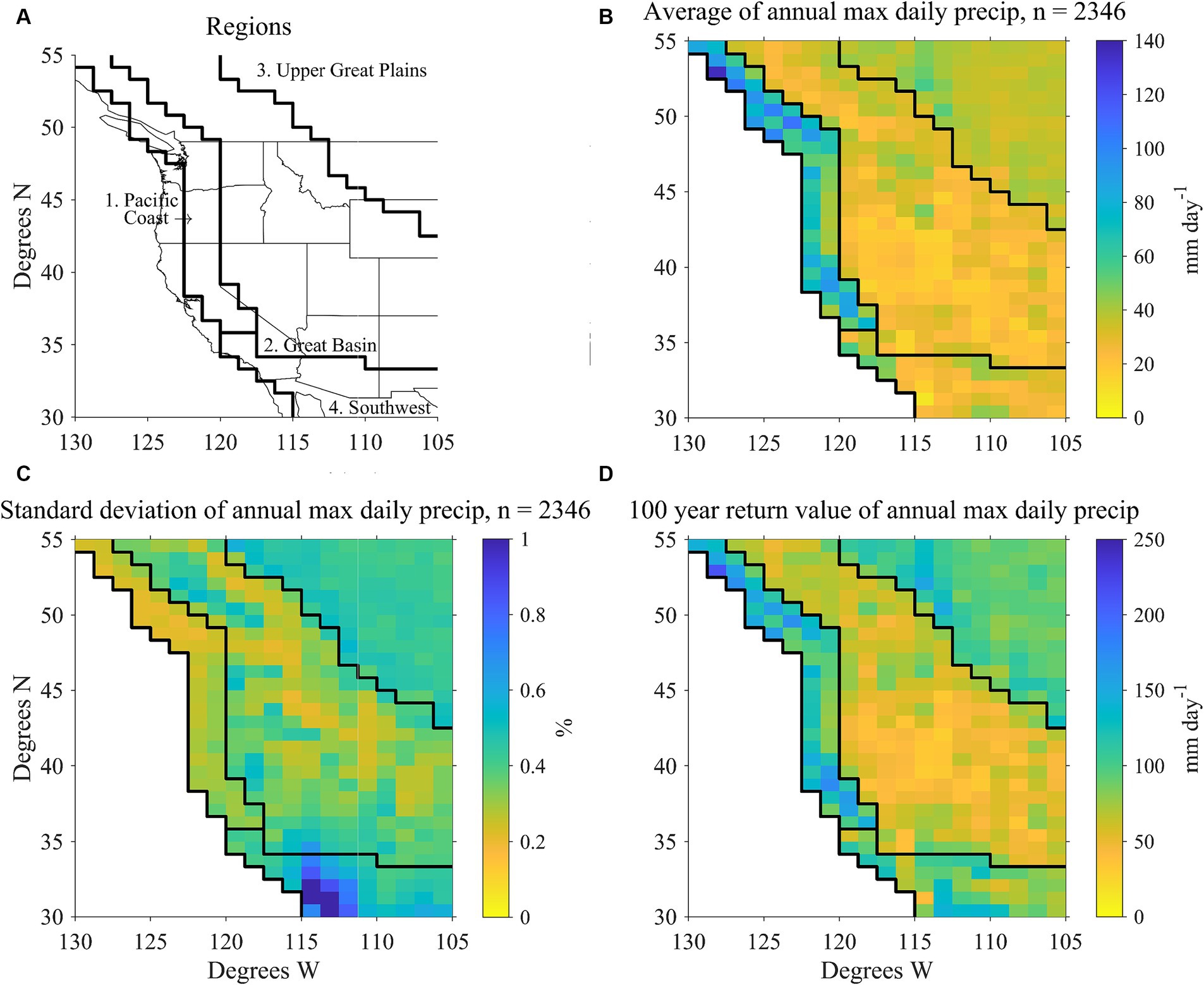
Figure 1. (A) Boundaries of the four homogenous regions. (B) Average of annual maximum of daily precipitation (mm day⁻¹) from 2,346 simulations. (C) Normalized ensemble standard deviation of annual maximum of daily precipitation (%). (D) 100-year return value of annual maximum of daily precipitation, calculated empirically (mm day⁻¹). Note the different color scales used in panels (B,D).

In the far Western U.S., extreme precipitation typically occurs during the winter months and in the Southwest U.S. precipitation typically occurs during the monsoonal season of July to September (Colorado-Ruiz and Cavazos, 2021), well after the April 1 start date of the simulations and allowing plenty of time for the atmospheric initial conditions in these atmosphere-only simulations to be forgotten. However, land surface moisture has memory for longer time scales than atmospheric process, and therefore likely retains some memory of the initial land conditions, which do not differ across the simulations, preventing the individual simulations from being truly independent. The strong seasonality of annual maximum precipitation in these two regions strengthens both the stationarity and identically-distributed assumptions. In other regions, where extreme precipitation can occur in any season, annual maximum samples may not be identically-distributed as they are the results of different storm processes, i.e., strong winter storms are different than strong summer storms.

4 Regional properties of Western U.S. and Southwestern Canada annual maximum daily precipitation

Statistical properties of precipitation in the Western U.S. and Southwestern Canada vary greatly across the region. We divide the domain into four contiguous regions based on similarities in the mean, variability and extremes of annual precipitation maxima and have labeled them as (1) Pacific Coast, (2) Great Basin, (3) Upper Great Plains, and (4) Southwest (Figure 1A). Annual-maximum daily precipitation averaged across the 2,346 ensemble members is shown in Figure 1B, its interannual standard deviation normalized by that average is shown in Figure 1C; and its 100-year return value (calculated empirically as discussed below) is shown in Figure 1D. All regional results in this paper are first calculated at individual grid cells before aggregating regionally. Regional boundaries are drawn such that the regions are relatively homogenous in the statistical properties (center and spread) of extreme precipitation (Table 1) and represent four different classes of extreme precipitation behavior. The Pacific Coast region, where most precipitation occurs in the winter months, has both large average annual maxima and return values but low interannual variability of annual maxima compared to the other regions. The semi-arid Great Basin region has low values of all three of these extreme precipitation metrics. The Upper Great Plains region, where daily precipitation maximum occurs in the summer months, has low values of average annual maxima but moderate interannual variability and high return values. The desert Southwest region has low average annual maxima but high interannual variability and return values.

Table 1

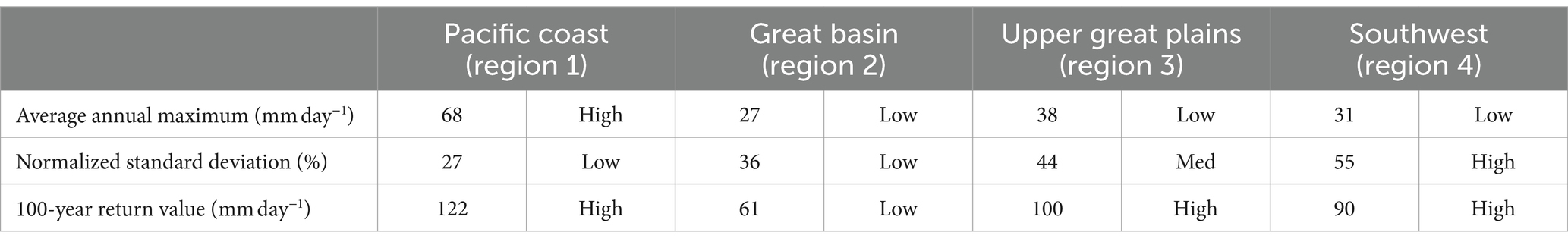
Table 1. Summary of regional properties of the annual maximum daily precipitation as obtained from all 2,346 samples.

5 A comparison of return value uncertainty from non-parametric and parametric methods

In this section, we use all 2,346 simulations to compare three methods of estimating long-period return values of daily precipitation at each grid cell: empirical, GEV using maximum likelihood estimation (MLE), and GEV using L-moments. The empirical method is nonparametric and the GEV methods are parametric. Maximum likelihood estimates of the GEV parameters are calculated using the MATLAB function gevfit. L-moments estimates of the GEV parameters are calculated using the FORTRAN routines supplied by Hosking and Wallis (1997). For both parametric GEV methods, after the parameters are estimated the return value is calculated using the MATLAB function icdf with the distribution name ‘Generalize Extreme Value’ for the MLE methods and directly from Equation 3 using the fitted parameters for the L-moments method. Regional averages of return value best estimates and their uncertainties using these two methods are compared in Figure 2 to estimates made empirically (Makkonen, 2006) for each of the four regions for return periods ranging from 20 to 1,000 years. The error bars in Figure 2 are obtained via a bootstrap with replacement scheme as described below and are averaged over each grid cell within the regions. Note that the y-axes differ for each region. Empirical estimates are simply calculated by taking the percentile values corresponding to return periods. With the exception of the Southwest region at return periods of 100 years or longer, there is effectively no difference between the best estimate of the two parametric methods and very little difference from the empirical best estimate. The high variability of the annual maximum precipitation in the Southwest region and its large return value relative to the average daily maximum (Figure 1 and Table 1) sets it apart from the other regions and methodological uncertainty in return value estimates is much higher in such desert regions even with very large extreme sample size.

Figure 2

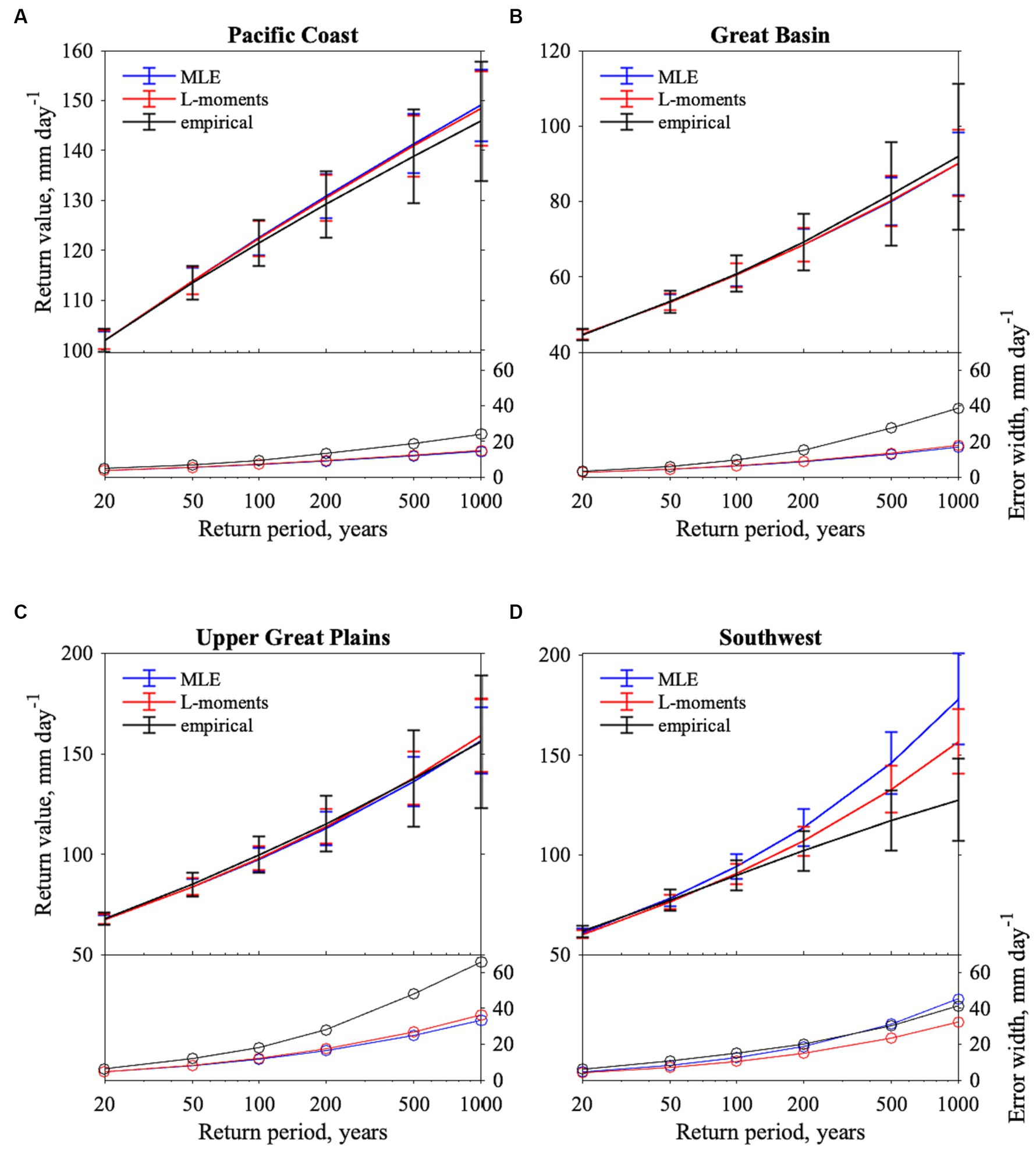
Figure 2. Regional average return value estimates made empirically (black), using MLE estimates of GEV parameters (blue), and using L-moments estimates of GEV parameters (red) for return periods of 20, 50, 100, 200, 500, and 1,000 years in four regions and using all 2,346 samples. Error bars are the regional average 2.5 and 97.5 percentiles of 500 bootstrap samples. The lower half of each panel shows the width of the error bars in mm day⁻¹. Data from all 2,346 simulations are used. The y-axes have different scales for each region in the upper half of each panel, but are consistent for the lower half of each panel. (A) Pacific Coast, (B) Great Basin, (C) Upper Great Plains, (D) Southwest.

The error bars show the 95% confidence interval of estimated return values, calculated as the 2.5th and 97.5th percentiles of 500 nonparametric bootstrap samples of size 2,346. “Best estimates” in Figure 2 and following figures indicate the estimate obtained by fitting the actual simulated datasets. This method of estimating uncertainty is compared to other methods in Section 7. For clarity, the width of these error bars is shown again in the lower half of each panel in Figure 2 as a function of return period for each method, this time with consistent y-axes.

In the Southwest region for long return periods there are differences in the bootstrap-estimated uncertainties between the two GEV methods, as there are with the return value estimates themselves. The apparent agreement in uncertainty estimates between the empirical and MLE in the Southwest is likely coincidental as the return value estimates are so different. We note that in the Southwest region at return periods of 200 years or longer, some return value estimates fall outside the confidence intervals of the other methods illustrating that methodological choices in this difficult region are important.

In the Upper Great Plains, Pacific Coast, and Great Basin regions, the uncertainties associated with both GEV parametric estimation methods are nearly identical at all return periods considered. However, the empirical uncertainty estimates are consistently higher in these regions than those of the parametric methods. We also note that return value estimates in these three regions are within the confidence intervals of each method over this range of return periods, indicating that discrepancies across methods are less important than sampling uncertainty even with these large sample sizes, except for very long return periods in the desert Southwest. Do these lower uncertainty estimates but consistent return value estimates demonstrate increased confidence for the parametric methods over an empirical method for very large samples? Indeed, there is added information in the GEV methods, that of a presumed underlying distribution for the annual maxima. This additional information imposes constraints on both the point estimate of return values and their confidence intervals even for the large data set size considered here. When extrapolating to return times past the duration of the time series, this effect would be larger and depend both on data set size and the degree of extrapolation. However, if the assumptions of the extreme value method are not satisfied by the data sample then an empirical approach, without these assumed constraints, would be more justified than a parametric approach. Of particular concern for annual maximum precipitation are the GEV requirements both of underlying i.i.d. and the shortness of the block size (Ben-Alaya et al., 2020). While we cannot know the true uncertainty for the full sample of 2,346 values, we show below that the GEV distribution is indeed well calibrated for small samples of this dataset for three of the four regions. However, the Southwest stands out from the other three regions in that there are substantial differences in long period return values obtained from all three methods, even the two parametric approaches. This desert region, characterized by low annual average precipitation but high variability and occasional intense monsoons illustrates that bias arising from methodological choices can significantly contribute to the overall uncertainty in long period return values.

The upward curvature of return value with increasing return period (i.e., its second derivative is positive) indicates that the fitted distributions averaged over each region, except the Pacific Coast, obtained from either the MLE and L-Moments methods are unbounded (ξ > 0), even for this very large sample of 2,346 annual values. As a return value of infinity for infinite return periods is clearly unphysical, a positive shape parameter of a fitted GEV distribution may indicate that it may not be appropriate estimating very long period return values or the upper bound on precipitation (Kunkel et al., 2013).

6 Return value uncertainty due to sample size for two parametric GEV methods

As a practical matter, observed or modeled daily climate datasets rarely span thousands of years. In this section, we take advantage of the large sample introduced in Section 5 to investigate the uncertainty of return value estimates as a function of shorter sample sizes for the two parametric GEV methods, still considering only a single method for uncertainty quantification. We did not consider empirical methods in this section. We divide the entire 2,346-member sample into subsamples of lengths, N (varying between 25 and 200) to construct n = integer(2,346/N) independent subsamples. For instance, there are n = 23 independent 100-member samples contained in the available data. For each sample, we calculate return values using the both the L-moments (solid) and MLE (dashed) procedures for return periods of 20, 50, 100, and 200 years and calculate the normalized standard deviation for each method across the n samples for each subsample length N, as shown in Figure 3. Normalization of the standard deviation by the averaged return value is done to permit comparison across the regions. This method of calculating uncertainty is referred to as the “true uncertainty” in Section 5 where we compare different uncertainty estimation techniques as it exploits all or nearly all of the available data.

Figure 3

Figure 3. Regional average uncertainty associated with GEV estimate of extreme precipitation value for sample sizes of 25–200. Uncertainty is standard deviation of the samples of estimates (see text), normalized by the GEV estimate of precipitation for the given region and return period. Uncertainties for both MLE (dashed) and L-moments (solid) estimates of precipitation extreme values are calculated for 20-year return period (black), 50-year return period (blue), 100-year return period (red), and 200-year return period (green). (A) Pacific Coast, (B) Great Basin, (C) Upper Great Plains, (D) Southwest.

As expected, the normalized standard deviation decreases with increasing sample size for both GEV parameter fitting methods, although rather slowly after the sample size exceeds the return period. The L-moments estimates have lower variation than the MLE estimates, especially for the smaller sample sizes. Hosking and Wallis (1997) showed that L-moments can be more efficient than MLE for small and moderate sample sizes, and Figure 3 suggests that such is the case for simulated Western U.S. and Southwestern Canada precipitation. This lower variance of L-moments estimates has been independently established in other studies.

The Pacific Coast region, with high long-period return values compared to a high average annual precipitation maximum and low interannual variability exhibits the smallest variations in return value estimates with sample size. Hence, both fitting methods are similar at sample sizes greater than 50. As in the previous section, the largest normalized standard deviations are in the Southwest region, as are the differences between L-Moments and MLE uncertainties. Uncertainty in the Upper Great Plains and Great Basin regions are similar to each other in Figure 3 despite their differences in statistical properties stated in Table 1.

The preceding analysis shows that return value uncertainty depends on both sample size and the return period (Figure 3). For a given sample size, uncertainty increases with return period. For a given return period, uncertainty increases as sample size decreases. To explore how these two effects interact, we present a measure of uncertainty as a function of the expected value of the number of extreme events in a sample. The expected value is the ratio of sample size to return period. For example, an expected value of two means that the sample size is twice as long as the return period (e.g., the expected value is two if the sample size is 200 for 1-in-100-year return period and if the sample size is 40 for 1-in-20-year return period).

Figure 4 shows the uncertainty as a function of the expected number of extreme events. Figure 4 is created by replicating Figure 3 except sample size is divided by the return period to get the expected number of extreme events. As shown in Figure 4, we find that for a given expected value, longer return periods (larger sample sizes) yield lower uncertainty than shorter return periods (smaller sample sizes). For example, for an expected value of 2 events, the uncertainty for the 1-in-100 year GEV estimate (sample size of 200) is smaller than for the 1-in-50 year GEV estimate (sample size of 100) which is smaller than the 1-in-20 year GEV estimate (sample size of 40). This indicates that the uncertainty in GEV estimate depends not only on the expected number of extreme events, but also on the sample size itself. Intuitively, this makes sense as we expect additional sample data to better constrain GEV parameters. Figure 4 also sheds insight into the additional uncertainty incurred by fitting a GEV using MLE techniques instead of L-moments techniques. Where the two GEV estimates converge depends on both sample size and on return period. At longer return periods, convergence occurs at lower expected values but higher sample sizes than shorter return periods.

Figure 4

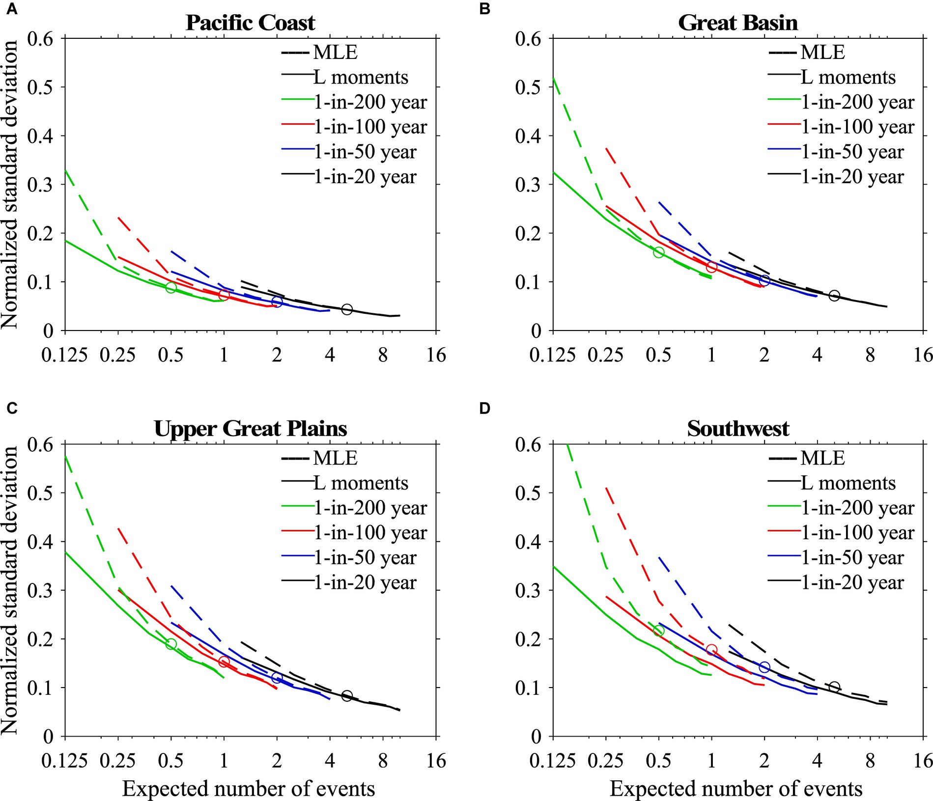
Figure 4. As in Figure 3 except regional average standard deviation is plotted as a function of the expected number of extreme events. The expected number of extreme events is the sample size divided by the return periods: 20 years (black), 50 years (blue), 100 years (red), and 200 years (green). Open circles denote MLE estimates of uncertainty with a bootstrap sample size of 100. (A) Pacific Coast, (B) Great Basin, (C) Upper Great Plains, (D) Southwest.

7 Different methods of estimating return value uncertainty

In this section, we compare various methods of estimating uncertainty. In Section 6 we were able to calculate the approximately “true” uncertainty by dividing the entire 2,346-member sample into ensembles of smaller sample sizes using all available data. In most practical applications, the task at hand is to estimate uncertainty from a single sample of smaller size N. Here, we have identified three practical methods of estimating uncertainty from smaller samples and compare to the true uncertainty as presented in Figure 3.

The first method is a standard non-parametric bootstrap with 500 generated draws similar to that used in Figure 2. Each of the 500 bootstrap draws of length (N = 20, 50, 100, 200 years) use a sampling scheme with replacement. The second is a parametric bootstrap constructed by first fitting the original data set to a GEV distribution (in this case by the MLE method), then generating 500 bootstrapped samples of similar lengths with a random number generator distributed according to that fitted GEV distribution (Efron and Tibshirani, 1994; Hosking and Wallis, 1997). A third approach is to use the delta method, which provides a formula for the asymptotic standard error of a function of maximum likelihood estimates (and is hence only applicable to the MLE approach). This formula (also presented in Equation 3.10 in Section 3.3.3 of Coles, 2001) propagates uncertainty in the GEV parameters (along with the degree of their co-variance) to corresponding uncertainty in the return values; note that this calculation can be done much more quickly than the bootstrap given that it is based on the raw input data and no additional resampling is required. We chose these three methods as they are straightforward and thus commonly used but we note that other uncertainty estimation techniques are also available including the profile likelihood method (Coles, 2001) or a full Bayesian implementation. Figure 5 compares the three methods to the true normalized standard deviation of estimated 200-year return values as a function of sample size for the four regions for results from the MLE fitted GEV distributions as calculated in Figure 4.

Figure 5

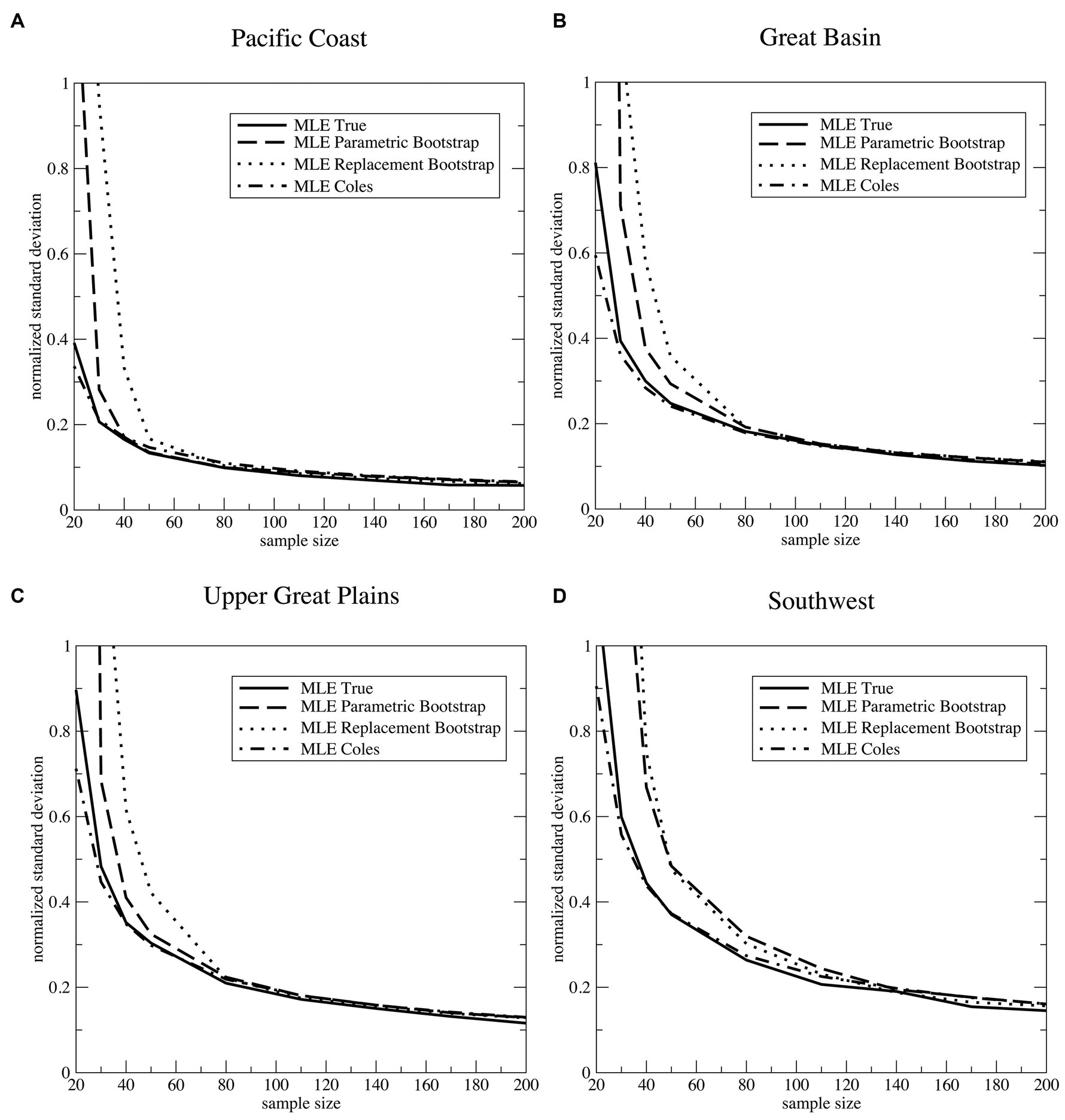
Figure 5. Four different estimates of normalized regional average uncertainty for the 200-year return value of annual maximum daily precipitation as fit by the MLE technique averaged over each of the four regions defined in Figure 1. Solid line: “True” uncertainty obtained by division of the entire dataset into 2,346/N samples as in Figure 3. Dashed line: The parametric bootstrap method of Hosking and Wallis (1997). Dotted line: A non-parametric bootstrap by a replacement method. Dashed-dotted line: Delta method of Coles (2001). (A) Pacific Coast, (B) Great Basin, (C) Upper Great Plains, (D) Southwest.

While all three of the approximate methods approach the true variance with increasing sample sizes, the delta method converges to it much faster. At the smallest sample sizes, the delta method slightly underestimates the true uncertainty, but both bootstrap methods substantially overestimate it. Of the two bootstrap methods, the non-parametric replacement sampling scheme estimates larger uncertainty than the parametric random number scheme except in the Southwest, where the two bootstrap uncertainties are about the same.

8 Uncertainty at much larger sample sizes

We showed in Section 7 that in the limit of large sample size, four different methods of estimating the normalized standard error converge to the same curves, whether the standard error is calculated as the standard deviation of estimates based on all available data, resampling (either parametrically or non-parametrically), or using asymptotic statistical theory (i.e., the delta method).

As plotted on linear scales in the previous figures, one might erroneously conclude that the uncertainty does not converge to zero with infinite sample size and that some sort of residual uncertainty underlies extreme precipitation. To further investigate convergence behavior beyond the available 2,346 simulations, we repeated the bootstrap procedure on idealized datasets of up to length N = 1,000,000 generated from presumed GEV distributions of μ = 0, σ = 1, and ξ = −0.2, 0.0, 0.2. (Note for the actual climate model data, the average of the shape parameter is ξ = −0.05 for the Pacific region, ξ = 0.10 for the Great Basin, ξ = 0.16 for the Upper Great Plains and ξ = 0.18 for the Southwest). Figure 6 shows the normalized standard deviation of these prescribed data sets on a log–log plot revealing that it is always decreasing with increasing sample size N regardless of whether the parent GEV distribution is bounded or not. The slope of all the lines in Figure 6 is −0.5, regardless of the shape parameter ξ and return period. Only the intercepts of these lines are controlled by shape parameter ξ and return period. Because of the normalization, these lines are independent of the scale parameter, σ. In hindsight, this behavior should be obvious as the empirical standard deviation across a large number of samples, n, is asymptotically equivalent to the true standard error, which scales with the inverse of the square root of the sample size, N, based on the Cramér-Rao lower bound.

Figure 6

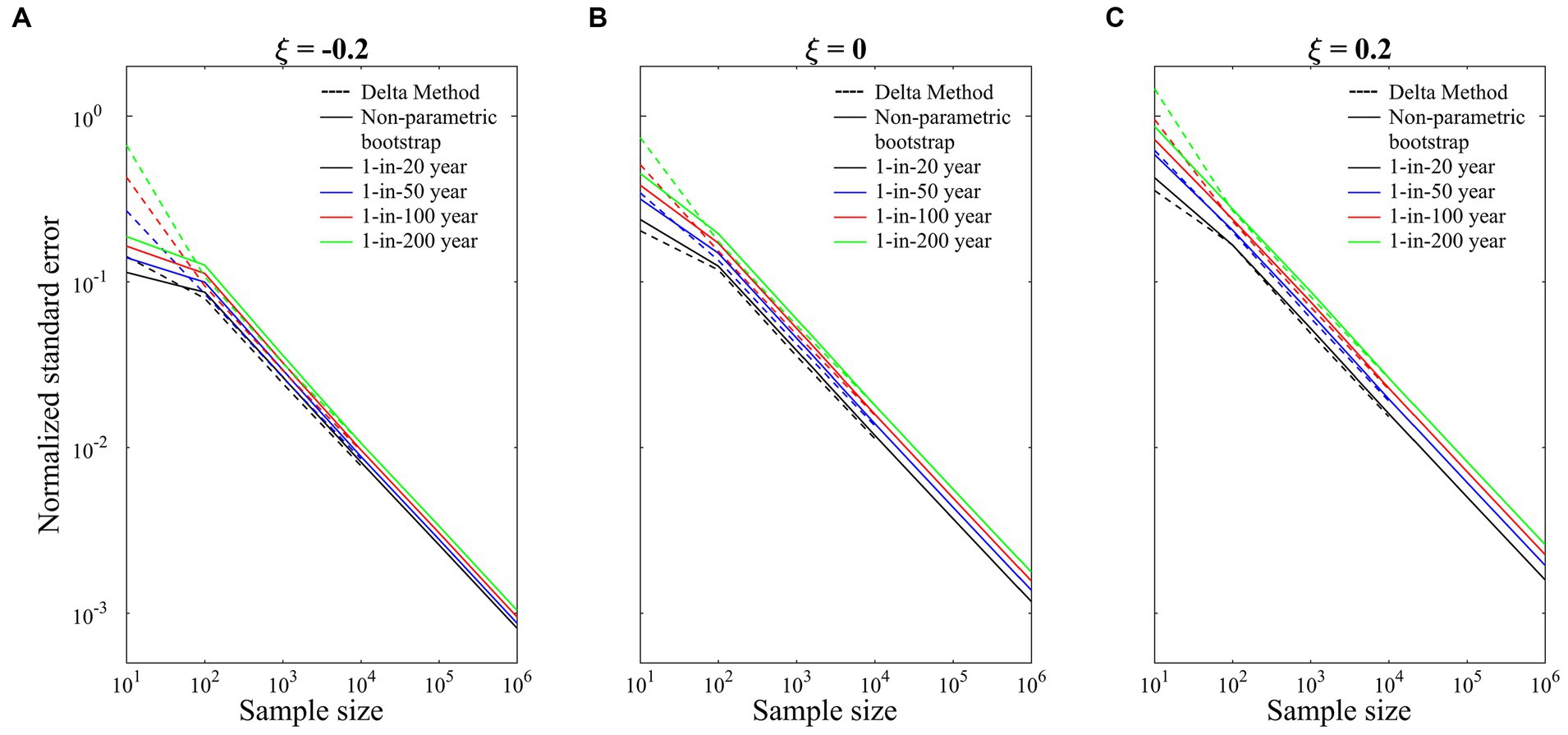
Figure 6. Normalized standard error of return value estimates for sample sizes ranging from 10 to 1,000,000, for artificial data drawn from GEV distributions that are (A) bounded, ξ = −0.2, (B) unbounded but with exponential tail ξ = 0, and (C) unbounded with polynomial tail, ξ = 0.2. Results are shown for both the Delta method as well as the nonparametric bootstrap.

9 Discussion and conclusion

Before summarizing our recommendations for practitioners, we disclose a number of caveats about the results in this paper. The experimental design of a large number of simulations of a single year does not contain all of the low frequency climate variability (Zhang et al., 2010). Hence, while Figures 2–6 are useful for comparing methodologies, they only characterize the uncertainty of extreme values of a single year generated by HadAM3-N144. Uncertainty in extreme values of longer duration datasets from this model would thus be larger due to internal variability. Second, our choice for block size is the annual maxima of daily precipitation. While very common in the literature (Sillmann et al., 2013), a single year is not a large enough block to avoid biases when extrapolating into the deep upper tail (Ben-Alaya et al., 2020). While there are good physical reasons to consider the extreme precipitation of each season separately (Risser et al., 2018), such blocks would be even smaller. Since it does not precipitate every day in a season, this source of bias is worse for extreme precipitation compared to temperature. This lack of max-stability in seasonal or annual maxima is further exacerbated when considering sub-daily extreme precipitation (Ben-Alaya et al., 2020).

Nonetheless, the results of this study permit several recommendations. The first recommendation, from Section 5, is that even for very large ensembles, it is worth performing GEV analyses to reduce uncertainty in estimating long-period return values rather than simply calculating percentiles and the empirical uncertainty therein, provided the assumptions underlying GEV theory are appropriate.

A second recommendation, involving the choice of GEV parameter fitting methods has more caveats. In the stationary case presented here, return value uncertainty converges faster for the L-moments method than for the MLE method as expected from its initial derivations (Hosking et al., 1985). While variance estimates are lower for L-Moment, MLE methods may exhibit less bias in precipitation extremes (Vivekanandan, 2018). However, MLE methods sometimes fail to converge even for large datasets such as used here (Nerantzaki and Papalexiou, 2022), or may produce unrealistic shape parameters for small samples (Martins and Stedinger, 2000). L-moments generally provide results in such situations (although possibly more biased). Although not widely utilized by climate data analysts, a Generalized Maximum Likelihood Estimator (GLM) combines both these methods to reduce variance compared to MLE at the same time reducing bias compared to L-moments by utilizing a Bayesian prior distribution to the shape parameter to reasonable values (Martins and Stedinger, 2000; Ailliot et al., 2011). However, widespread adoption of GLM by climate analysts would require inclusion of the method in publicly available software tools.

However, extreme precipitation from observations or longer realistically forced historical and future projection climate model simulations are non-stationary due to the effects of climate change. While there are non-stationary MLE formalisms and software allowing the use of covariates to incorporate both relevant external forcings and internal modes of variability (Risser et al., 2021, 2023), there are no such practical non-stationary implementations for L-moments. Hence, in order to use L-moments on such datasets, some studies have presumed a quasi-stationary assumption by temporally sub-setting the dataset into segments of one or two decades, as significantly longer time series would have a detectable trend (Kharin et al., 2013). As Figure 3 reveals, the sampling uncertainty for such small samples can be very large when estimating long period return values. Although this uncertainty can be significantly reduced by combining the multiple realizations of climate model ensemble simulations to expand the sample size, it cannot be reduced for observations in this manner. As a practical matter, despite the greater efficiency of the L-moments method, the covariate MLE methods (Coles, 2001) and the usage of much longer time series would generally be preferable, except for very large ensembles (Tebaldi and Wehner, 2018).

Indeed, the recent development of very large ensembles of both coupled ocean atmosphere models (Kay et al., 2015; Smith et al., 2022) and standalone atmosphere models (Stone et al., 2019) permits more flexibility in the choice of extreme value estimation techniques. For instance, the single year methodology shown in the previous sections can be replicated by constructing samples for each individual simulated year using all the realizations. Figure 7 shows a time series of estimated 100 year return values of annual maximum daily precipitation from the Climate of the 20th Century Plus (C20C+) simulations of the Community Atmospheric Model version 5 at a resolution of approximately 0.9^o × 1.25^o, similar to HadAM3-N144 (Wehner et al., 2018; Stone et al., 2019). This stand-alone atmospheric model dataset consists of 100 individual realizations, perturbed at initialization, forced under the AMIP protocols (Gates, 1992). Return values and uncertainties were calculated separately for each year with a sample size of 100 using L-moments. Standard deviation was calculated by the parametric bootstrap method (Efron and Tibshirani, 1994; Hosking and Wallis, 1997). Figure 7 reveals that simulated trends in the 100 year return value averaged over the four western North American regions are small over this 23 year period compared to sampling uncertainty, supporting the 20 year quasi-stationary assumption mentioned above. However, this may not be the case in other regions nor over longer periods experiencing larger anthropogenic forcing. Also, we note that in this AMIP experiment each realization is simulated not only with the same external forcings but also with identical modes of oceanic natural variability via the prescribed sea surface temperatures. Similar large ensembles from coupled ocean–atmosphere models would differ each year in their ocean states. Hence, the stationary assumption required by L-moments may not be satisfied and non-stationary MLE methods as discussed below may be more appropriate.

Figure 7

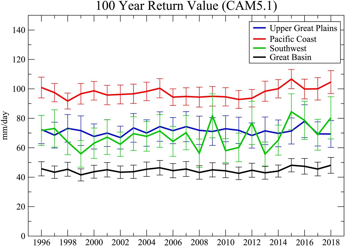
Figure 7. Regionally averaged 100 year return values and standard deviations of annual maximum daily precipitation as simulated by the Community Atmospheric Model (CAM5.1) and obtained by the L-Moments method. Standard deviation calculated by the parametric bootstrap method (Units = mm/day).

While we have not investigated non-stationary covariates in this study, we comment on them here as previous work reveals how useful they can be in reducing return value uncertainty by allowing increased sample size over the quasi-stationary assumption. While it is tempting to simply use time itself to represent non-stationarity due to anthropogenic forcing, other covariates more physically represent these processes. For instance, radiative forcing has been shown to be proportional to the logarithm of greenhouse gas equivalent carbon dioxide concentration (Etminan et al., 2016) and has been used to represent part of the human component of non-stationarity in event attribution studies (Risser and Wehner, 2017). Land use changes and aerosol and ozone concentrations as well as volcanic and solar irradiance may also be suitable covariates representing forcings external to the climate system. It is also well established that natural, internal modes of variability such as El Niño, the Atlantic Meriodional Mode, the Pacific Decadal Oscillation can influence extreme precipitation and/or temperature and can serve as useful covariates either globally or locally (Risser et al., 2021, 2023). While temporal covariates have been used to represent non-stationarity in both the location and scale parameters, it is prudent to investigate whether or not goodness of fit is improved by their usage, as each covariate increases the number of fitting parameters. For example, Zhang et al. (2024) found that adding covariates without enforcing spatial coherence in their estimates worsened GEV fits relative to a simple time trend model illustrating that covariate choice is not always straightforward. It has been suggested that non-stationarity should also be considered in the shape parameter (Richard Smith, private communication) but as uncertainty in the shape parameter is generally high, the usefulness of this suggestion has not been yet demonstrated to be necessary. Adding additional covariates increases the degrees of freedom and may not improve the quality of fitted distributions, especially if the uncertainty in the covariate terms includes zero. Careful assessments of fit quality and information content are recommended. However, recent work in the rapidly developing field of spatial statistics may alleviate this problem. By exploiting the similarities in nearby observations or model grid cells, effective sample sizes can be increased (Risser and Wehner, 2020; Zhang et al., 2022). Hence, our second recommendation is that for observations and small ensemble simulations, judicious choice of covariates may reduce uncertainty by allowing increased sample sizes.

Our third recommendation is that for large ensemble simulations, forgoing covariates and presuming a quasi-stationary assumption over short analysis periods may be simpler and computationally more efficient.

If a quasi-stationary assumption is made, Peaks over Threshold (POT) methods of constructing precipitation maxima may be a more efficient usage of the available data than block maxima. However, declustering should be applied as high values may occur sequentially and lead to a low bias in estimated return values (Coles, 2001). We note that similar to the arbitrary choice of yearly as a block size, threshold choice is similarly arbitrary and presents a tradeoff between extremal data set size and the requisite asymptotic assumption of extreme value theory. In the non-stationary case, while it is possible to introduce covariates into the Generalized Pareto Distribution (Mackay and Jonathan, 2020), experience is limited.

There is a point of diminishing returns in the reduction of uncertainty with increasing sample size. Although uncertainty goes to zero for any shape parameter and the rate of decreasing uncertainty asymptotes at very large sample size for any return period (Figure 7), there are stark differences at the moderate sample sizes both regionally and at different return periods (Figure 3). The bounded distributions in the Pacific Coast region flatten at significantly smaller samples than do the very heavy tailed distributions of the Southwest region. The fourth recommendation is when designing large climate model ensemble simulations, that consideration of uncertainty behavior in the variables and regions of interest be taken into account. In the absence of previously performed large ensembles, estimation of uncertainty obtained by segmenting long stationary control runs can provide guidance. Previous work, presuming quasi-stationarity over 11 year periods suggests that 20 realizations (effective sample size of 220) may suffice (Tebaldi et al., 2021).

The fifth recommendation is that in the limit of reasonably large samples, any method of estimating return value uncertainty is equivalent but the delta method provides a more accurate estimate of the uncertainty at smaller sample sizes obtained from the MLE method, and is substantially computationally simpler for any sample size. However as a cautionary note, the delta method can underestimate uncertainty if the sample size is very small compared to the return value. The two bootstrap methods considered here tend to overestimate the true internal variability at such small sample sizes (Figure 5). But as pointed out in (Paciorek et al., 2018), bootstrap methods are known to perform poorly both theoretically and in practice when examining tails of distributions. Paciorek et al. (2018) also discuss estimating the uncertainty in the ratio of return times as the climate changes and present additional recommendations for this related but more specialized issue.

The sixth recommendation comes from Figure 5 that shows that using the number of expected events of a given rarity to estimate optimal sample size may be misleading in GEV analyses and is not a recommended best practice. We find that for shorter return periods more expected events in the sample are required to estimate return values to within a specified normalized uncertainty.

Finally, although we have not investigated systematic bias in return value estimates, we will make a few comments. The principal sources of return value bias are (a) the sub-sampling of the parent dataset to construct an extreme value sample, (b) the validity of a max-stable assumption, (c) the length of the record, and (d) selection bias.

As discussed above, it is critical that extreme value samples be independent and identically distributed (i.i.d). In many regions annualized precipitation extrema would not be i.i.d. due to the seasonality of precipitation (Wehner, 2004, 2013; Wehner et al., 2021). Furthermore, extreme precipitation differs by storm type (Kunkel et al., 2012) and an extreme value sample should be further sub-sampled using storm trackers (Prabhat et al., 2012; Ullrich and Zarzycki, 2017) or some other technology. We recognize that this is not a standard practice but recommend it as an aspiration.

Extreme value theory dictates that the sample be representative of the far tail of the distribution. To be within this asymptotic or max-stable regime requires both large parent data size and that it be sampled correctly (Ben-Alaya et al., 2020) tested for max-stability by testing the convergence of fitted shape parameters of hourly maxima as a function of block size finding strong variations across North America. At locations where annual maxima were not max-stable, fitted distributions also demonstrated poor quality of fit in the upper tail. At two locations considered where shape parameter stabilized at block sizes of 5 years or less, return value bias was rather small. But at a location where shape parameter increased (decreased) with block size, estimated return values were biased low (high). We note that the same issue is faced with choice of threshold in Generalized Pareto extreme value methods. While threshold plays the same role as block size in determining max-stability, it may be more intuitive to some.

It is a common practice in event attribution studies to perform “out of sample” statistical analyses where the event in question (often the maximum value in the observations) is excluded. It has recently been pointed out that this can introduce a selection bias (Miralles and Davison, 2023; Zeder et al., 2023). However, it can be the case that the maxima in question can be far outliers and cause very poor quality of fit for the rest of the extreme value sample data if included in the fitting data (Bercos-Hickey et al., 2022) casting doubts on the validity of the attribution statements. These recent studies were motivated by the 2021 Pacific Northwest heatwave (Philip et al., 2022). This source of selection bias is likely to depend on whether the fitted GEV distribution is sharply bounded as for temperature or exhibits a long or heavy tail as for precipitation and much more work needs to be done.

Hence our final recommendation is that whatever choice of data set size, sampling method or max-stability criteria, those estimating long period return values from limited data sets must be aware of the bias-variance tradeoffs. High confidence in an estimate may not necessarily be better. Caution would suggest that multiple lines of testing be performed as the data allows.

Data availability statement

Original datasets are available in publicly accessible repositories: HadAM3-N144 model output data was obtained from the Seasonal Attribution Experiment and is available at https://www.climateprediction.net/projects/completed-project/hadcm3-and-other-models/seasonal-attribution-experiment/. Model output from the C20C+ experiments is available at https://portal.nersc.gov/c20c/. The original contributions presented in the study are also publicly available as follows: Codes to calculate the GEV are available at https://cran.r-project.org/web/packages/climextRemes/index.htmland https://github.com/CDAT/cdat. Annual and seasonal maximum precipitation data from the HadAM3-N144 experiments is available at https://portal.nersc.gov/archive/home/projects/cascade/www/frontier_GEV_max_precip.tar.

Author contributions

MW: Conceptualization, Investigation, Methodology, Software, Supervision, Visualization, Writing – original draft, Writing – review & editing. MD: Investigation, Software, Visualization, Writing – original draft, Writing – review & editing. MR: Investigation, Writing – review & editing. CP: Investigation, Writing – review & editing. DS: Writing – review & editing. PP: Data curation, Writing – review & editing.

Funding

The author(s) declare that financial support was received for the research, authorship, and/or publication of this article. This research was supported by the Director, Office of Science, Office of Biological and Environmental Research of the U.S. Department of Energy under Contract No. DE340AC02-05CH11231. Support from the Regional and Global Model Analysis program as part of the Calibrated and Systematic Characterization, Attribution, and Detection of Extremes (CASCADE) project is gratefully acknowledged. This document was prepared as an account of work sponsored by the United States Government. While this document is believed to contain correct information, neither the United States Government nor any agency thereof, nor the Regents of the University of California, nor any of their employees, makes any warranty, express or implied, or assumes any legal responsibility for the accuracy, completeness, or usefulness of any information, apparatus, product, or process disclosed, or represents that its use would not infringe privately owned rights. Reference herein to any specific commercial product, process, or service by its trade name, trademark, manufacturer, or otherwise, does not necessarily constitute or imply its endorsement, recommendation, or favoring by the United States Government or any agency thereof, or the Regents of the University of California. The views and opinions of authors expressed herein do not necessarily state or reflect those of the United States Government or any agency thereof or the Regents of the University of California. This work used resources at the National Energy Research Supercomputer Center (NERSC) at the Lawrence Berkeley National Laboratory. This material is also based upon work supported by the NSF National Center for Atmospheric Research, which is a major facility sponsored by the U.S. National Science Foundation under Cooperative Agreement No. 1852977.

Acknowledgments

The authors thank Hari Krishnan for help with implementing software. MD acknowledges the support of the Department of Energy’s Science Undergraduate Laboratory Internship (SULI) program.

Conflict of interest

The authors declare that the research was conducted in the absence of any commercial or financial relationships that could be construed as a potential conflict of interest.

Publisher’s note

All claims expressed in this article are solely those of the authors and do not necessarily represent those of their affiliated organizations, or those of the publisher, the editors and the reviewers. Any product that may be evaluated in this article, or claim that may be made by its manufacturer, is not guaranteed or endorsed by the publisher.

References

Ailliot, P., Thompson, C., and Thomson, P. (2011). Mixed methods for fitting the GEV distribution. Water Resour. Res. 47:W05551. doi: 10.1029/2010WR009417

Crossref Full Text | Google Scholar

Ben-Alaya, M. A., Zwiers, F. W., and Zhang, X. (2020). An evaluation of block-maximum-based estimation of very long return period precipitation extremes with a large ensemble climate simulation. J. Clim. 33, 6957–6970. doi: 10.1175/JCLI-D-19-0011.1

Crossref Full Text | Google Scholar

Bercos-Hickey, E., O’Brien, T. A., Wehner, M. F., Zhang, L., Patricola, C. M., Huang, H., et al. (2022). Anthropogenic contributions to the 2021 Pacific northwest heatwave. Geophys. Res. Lett. 49:e2022GL099396. doi: 10.1029/2022GL099396

Crossref Full Text | Google Scholar

Chen, C.-T., and Knutson, T. (2008). On the verification and comparison of extreme rainfall indices from climate models. J. Clim. 21, 1605–1621. doi: 10.1175/2007JCLI1494.1

Crossref Full Text | Google Scholar

Coles, S. (2001). An introduction to statistical modeling of extreme values. Berlin: Springer.

Google Scholar

Colorado-Ruiz, G., and Cavazos, T. (2021). Trends of daily extreme and non-extreme rainfall indices and intercomparison with different gridded data sets over Mexico and the southern United States. Int. J. Climatol. 41, 5406–5430. doi: 10.1002/joc.7225

Crossref Full Text | Google Scholar

Efron, B., and Tibshirani, R. J. (1994). An introduction to the bootstrap. New York: CRC Press.

Google Scholar

Embrechts, P., Klüppelberg, C., and Omas Mikosch, T. (1997). Modelling extremal events for insurance and finance. Springer, New York

Google Scholar

Etminan, M., Myhre, G., Highwood, E. J., and Shine, K. P. (2016). Radiative forcing of carbon dioxide, methane, and nitrous oxide: a significant revision of the methane radiative forcing. Geophys. Res. Lett. 43, 12,614–12,623. doi: 10.1002/2016GL071930

Crossref Full Text | Google Scholar

Gates, W. L. (1992). AN AMS CONTINUING SERIES: GLOBAL CHANGE--AMIP: the atmospheric model intercomparison project. Bull. Am. Meteorol. Soc. 73, 1962–1970. doi: 10.1175/1520-0477(1992)073<1962:ATAMIP>2.0.CO;2

Crossref Full Text | Google Scholar

Gervais, M., Tremblay, L. B., Gyakum, J. R., and Atallah, E. (2014). Representing extremes in a daily gridded precipitation analysis over the United States: impacts of station density, resolution, and gridding methods. J. Clim. 27, 5201–5218. doi: 10.1175/JCLI-D-13-00319.1

Crossref Full Text | Google Scholar

Gilleland, E., and Katz, R. W. (2016). extRemes 2.0: an extreme value analysis package in R. J. Stat. Softw. 72, 1–39. doi: 10.18637/jss.v072.i08

Crossref Full Text | Google Scholar

Hawkins, E., and Sutton, R. (2009). The potential to narrow uncertainty in regional climate predictions. Bull. Am. Meteorol. Soc. 90, 1095–1108. doi: 10.1175/2009BAMS2607.1

Crossref Full Text | Google Scholar

Hawkins, E., and Sutton, R. (2011). The potential to narrow uncertainty in projections of regional precipitation change. Clim. Dyn. 37, 407–418. doi: 10.1007/s00382-010-0810-6

Crossref Full Text | Google Scholar

Hosking, J., and Wallis, J. R. (1997). Regional frequency analysis. Cambridge: Cambridge University Press.

Google Scholar

Hosking, J. R. M., Wallis, J. R., and Wood, E. F. (1985). Estimation of the generalized extreme-value distribution by the method of probability-weighted moments. Technometrics 27, 251–261. doi: 10.1080/00401706.1985.10488049

Crossref Full Text | Google Scholar

Kay, J. E., Deser, C., Phillips, A., Mai, A., Hannay, C., Strand, G., et al. (2015). The community earth system model (CESM) large ensemble project: a community resource for studying climate change in the presence of internal climate variability. Bull. Am. Meteorol. Soc. 96, 1333–1349. doi: 10.1175/BAMS-D-13-00255.1

Crossref Full Text | Google Scholar

Kharin, V. V., Zwiers, F. W., Zhang, X., and Wehner, M. (2013). Changes in temperature and precipitation extremes in the CMIP5 ensemble. Clim. Chang. 119, 345–357. doi: 10.1007/s10584-013-0705-8

Crossref Full Text | Google Scholar

Kunkel, K. E., Easterling, D. R., Kristovich, D. A. R., Gleason, B., Stoecker, L., and Smith, R. (2012). Meteorological causes of the secular variations in observed extreme precipitation events for the conterminous United States. J. Hydrometeorol. 13, 1131–1141. doi: 10.1175/JHM-D-11-0108.1

Crossref Full Text | Google Scholar

Kunkel, K. E., Karl, T. R., Easterling, D. R., Redmond, K., Young, J., Yin, X., et al. (2013). Probable maximum precipitation and climate change. Geophys. Res. Lett. 40, 1402–1408. doi: 10.1002/grl.50334

Crossref Full Text | Google Scholar

Mackay, E., and Jonathan, P. (2020). Assessment of return value estimates from stationary and non-stationary extreme value models. Ocean Eng. 207:107406. doi: 10.1016/j.oceaneng.2020.107406

Crossref Full Text | Google Scholar

Makkonen, L. (2006). Plotting positions in extreme value analysis. J. Appl. Meteorol. Climatol. 45, 334–340. doi: 10.1175/JAM2349.1

Crossref Full Text | Google Scholar

Martins, E., and Stedinger, J. (2000). Generalized maximum likelihood GEV quantile estimators for hydrologic data. Water Resour. Res. 36, 737–744. doi: 10.1029/1999WR900330

Crossref Full Text | Google Scholar

Min, S.-K., Zhang, X., Zwiers, F. W., and Hegerl, G. C. (2011). Human contribution to more-intense precipitation extremes. Nature 470, 378–381. doi: 10.1038/nature09763

PubMed Abstract | Crossref Full Text | Google Scholar

Miralles, O., and Davison, A. C. (2023). Timing and spatial selection bias in rapid extreme event attribution. Weather Clim. Extremes 41:100584. doi: 10.1016/j.wace.2023.100584

Crossref Full Text | Google Scholar

Nerantzaki, S. D., and Papalexiou, S. M. (2022). Assessing extremes in hydroclimatology: a review on probabilistic methods. J. Hydrol. 605:127302. doi: 10.1016/j.jhydrol.2021.127302

Crossref Full Text | Google Scholar

Paciorek, C. J., Stone, D. A., and Wehner, M. F. (2018). Quantifying statistical uncertainty in the attribution of human influence on severe weather. Weather Clim. Extremes 20, 69–80. doi: 10.1016/j.wace.2018.01.002

Crossref Full Text | Google Scholar

Pall, P., Aina, T., Stone, D. A., Stott, P. A., Nozawa, T., Hilberts, A. G. J., et al. (2011). Anthropogenic greenhouse gas contribution to flood risk in England and Wales in autumn 2000. Nature 470, 382–385. doi: 10.1038/nature09762

PubMed Abstract | Crossref Full Text | Google Scholar

Philip, S. Y., Kew, S. F., van Oldenborgh, G. J., Anslow, F. S., Seneviratne, S. I., Vautard, R., et al. (2022). Rapid attribution analysis of the extraordinary heat wave on the Pacific coast of the US and Canada in June 2021. Earth Syst. Dynam. 13, 1689–1713. doi: 10.5194/esd-13-1689-2022

Crossref Full Text | Google Scholar

Pope, V., and Stratton, R. (2002). The processes governing horizontal resolution sensitivity in a climate model. Clim. Dyn. 19, 211–236. doi: 10.1007/s00382-001-0222-8

Crossref Full Text | Google Scholar

Prabhat, R., Rübel, O., Byna, S., Wu, K., Li, F., Wehner, M., et al. (2012). TECA: a parallel toolkit for extreme climate analysis. Proc. Comput. Sci. 9, 866–876. doi: 10.1016/j.procs.2012.04.093

Crossref Full Text | Google Scholar

Risser, M. D., Collins, W. D., Wehner, M. F., O’Brien, T. A., Paciorek, C. J., O’Brien, J. P., et al. (2023). A framework for detection and attribution of regional precipitation change: application to the United States historical record. Clim. Dyn. 60, 705–741. doi: 10.1007/s00382-022-06321-1

Crossref Full Text | Google Scholar

Risser, M. D., Paciorek, C. J., Wehner, M. F., O’Brien, T. A., and Collins, W. D. (2018). A probabilistic gridded product for daily precipitation extremes over the United States. Clim. Dyn. 53, 2517–2538. doi: 10.1007/s00382-019-04636-0

Crossref Full Text | Google Scholar

Risser, M. D., and Wehner, M. F. (2017). Attributable human-induced changes in the likelihood and magnitude of the observed extreme precipitation during hurricane Harvey. Geophys. Res. Lett. 44, 12,457–12,464. doi: 10.1002/2017GL075888

Crossref Full Text | Google Scholar

Risser, M. D., and Wehner, M. F. (2020). The effect of geographic sampling on evaluation of extreme precipitation in high-resolution climate models. Adv. Stat. Climatol. Meteorol. Oceanogr. 6, 115–139. doi: 10.5194/ascmo-6-115-2020

Crossref Full Text | Google Scholar

Risser, M. D., Wehner, M. F., O’Brien, J. P., Patricola, C. M., O’Brien, T. A., Collins, W. D., et al. (2021). Quantifying the influence of natural climate variability on in situ measurements of seasonal total and extreme daily precipitation. Clim. Dyn. 56, 3205–3230. doi: 10.1007/s00382-021-05638-7

Crossref Full Text | Google Scholar

Sillmann, J., Kharin, V., Zhang, X., Zwiers, F. W., and Bronaugh, D. (2013). Climate extremes indices in the CMIP5 multimodel ensemble: part 1. Model evaluation in the present climate. J. Geophys. Res. Atmos. 118, 1716–1733. doi: 10.1002/jgrd.50203

Crossref Full Text | Google Scholar

Smith, D. M., Gillett, N. P., Simpson, I. R., Athanasiadis, P. J., Baehr, J., Bethke, I., et al. (2022). Attribution of multi-annual to decadal changes in the climate system: the large ensemble single forcing model intercomparison project (LESFMIP). Front. Clim. 4:955414. doi: 10.3389/fclim.2022.955414

Crossref Full Text | Google Scholar

Stone, D. A., Christidis, N., Folland, C., Perkins-Kirkpatrick, S., Perlwitz, J., Shiogama, H., et al. (2019). Experiment design of the international CLIVAR C20C+ detection and attribution project. Weather Clim. Extremes 24:100206. doi: 10.1016/j.wace.2019.100206

Crossref Full Text | Google Scholar

Tebaldi, C., Dorheim, K., Wehner, M., and Leung, R. (2021). Extreme metrics from large ensembles: investigating the effects of ensemble size on their estimates. Earth Syst. Dynam. 12, 1427–1501. doi: 10.5194/esd-12-1427-2021

Crossref Full Text | Google Scholar

Tebaldi, C., and Wehner, M. F. (2018). Benefits of mitigation for future heat extremes under RCP4.5 compared to RCP8.5. Clim. Chang. 146, 349–361. doi: 10.1007/s10584-016-1605-5

Crossref Full Text | Google Scholar

Ullrich, P. A., and Zarzycki, C. M. (2017). TempestExtremes: a framework for scale-insensitive pointwise feature tracking on unstructured grids. Geosci. Model Dev. 10, 1069–1090. doi: 10.5194/gmd-10-1069-2017

Crossref Full Text | Google Scholar

Vivekanandan, N. (2018). Comparison of probability distributions in extreme value analysis of rainfall and temperature data. Environ. Earth Sci. 77:201. doi: 10.1007/s12665-018-7356-z

Crossref Full Text | Google Scholar

Wehner, M. F. (2004). Predicted twenty-first-century changes in seasonal extreme precipitation events in the parallel climate model. J. Clim. 17, 4281–4290. doi: 10.1175/JCLI3197.1

Crossref Full Text | Google Scholar

Wehner, M. (2010). Sources of uncertainty in the extreme value statistics of climate data. Extremes 13, 205–217. doi: 10.1007/s10687-010-0105-7

Crossref Full Text | Google Scholar

Wehner, M. F. (2013). Very extreme seasonal precipitation in the NARCCAP ensemble: model performance and projections. Clim. Dyn. 40, 59–80. doi: 10.1007/s00382-012-1393-1

Crossref Full Text | Google Scholar

Wehner, M., Lee, J., Risser, M., Ullrich, P., Gleckler, P., and Collins, W. D. (2021). Evaluation of extreme sub-daily precipitation in high-resolution global climate model simulations. Philos. Trans. R. Soc. A Math. Phys. Eng. Sci. 379:20190545. doi: 10.1098/rsta.2019.0545

PubMed Abstract | Crossref Full Text | Google Scholar

Wehner, M., Reed, K., Li, F., Prabhat, B., Bacmeister, J., Chen, C.-T., et al. (2014). The effect of horizontal resolution on simulation quality in the community atmospheric model, CAM5.1. J. Adv. Model. Earth Syst. 6, 980–997. doi: 10.1002/2013MS000276

Crossref Full Text | Google Scholar

Wehner, M., Stone, D., Shiogama, H., Wolski, P., Ciavarella, A., Christidis, N., et al. (2018). Early 21st century anthropogenic changes in extremely hot days as simulated by the C20C+ detection and attribution multi-model ensemble. Weather Clim. Extremes 20, 1–8. doi: 10.1016/j.wace.2018.03.001

Crossref Full Text | Google Scholar

Zeder, J., Sippel, S., Pasche, O. C., Engelke, S., and Fischer, E. M. (2023). The effect of a short observational record on the statistics of temperature extremes. Geophys. Res. Lett. 50:e2023GL104090. doi: 10.1029/2023GL104090

Crossref Full Text | Google Scholar

Zhang, L., Risser, M. D., Molter, E. M., Wehner, M. F., and O'Brien, T. A. (2022). Accounting for the spatial structure of weather systems in detected changes in precipitation extremes. Weather Clim. Extremes 38:100499. doi: 10.1016/j.wace.2022.100499

Crossref Full Text | Google Scholar

Zhang, L., Risser, M. D., Wehner, M. F., and O’Brien, T. A. (2024). Explaining the unexplainable: leveraging extremal dependence to characterize the 2021 Pacific Northwest heatwave, Revision in review at Journal of Agricultural, Biological, and Environmental Statistics. Preprint Available at https://arxiv.org/abs/2307.03688

Google Scholar

Zhang, X., Wan, H., Zwiers, F. W., Hegerl, G. C., and Min, S.-K. (2013). Attributing intensification of precipitation extremes to human influence. Geophys. Res. Lett. 40, 5252–5257. doi: 10.1002/grl.51010

Crossref Full Text | Google Scholar

Zhang, X., Wang, J., Zwiers, F. W., and Groisman, P. Y. (2010). The influence of large-scale climate variability on winter maximum daily precipitation over North America. J. Clim. 23, 2902–2915. doi: 10.1175/2010JCLI3249.1

Crossref Full Text | Google Scholar