 Philipp Heinrich
 Stefan Hagemann
 Ralf Weisse
 Lidia Gaslikova
95% of researchers rate our articles as excellent or good
Learn more about the work of our research integrity team to safeguard the quality of each article we publish.
Find out more
ORIGINAL RESEARCH article
Front. Clim. , 01 September 2023
Sec. Predictions and Projections
Volume 5 - 2023 | https://doi.org/10.3389/fclim.2023.1227613
The simultaneous occurrence of increased river discharge and high coastal water levels may cause compound flooding. Compound flood events can potentially cause greater damage than the separate occurrence of the underlying extreme events, making them essential for risk assessment. Even though a general increase in the frequency and/or severity of compound flood events is assumed due to climate change, there have been very few studies conducted for larger regions of Europe. Our work, therefore, focuses on the high-resolution analysis of changes in extreme events of coastal water levels, river discharge, and their concurrent appearance at the end of this century in northern and central Europe (2070–2099). For this, we analyze downscaled data sets from two global climate models (GCMs) for the two emissions scenarios RCP2.6 and RCP8.5. First, we compare the historical runs of the downscaled GCMs to historical reconstruction data to investigate if they deliver comparable results for northern and central Europe. Then we study changes in the intensity of extreme events, their number, and the duration of extreme event seasons under climate change. Our analysis shows increases in compound flood events over the whole European domain, mostly due to the rising mean sea level. In some areas, the number of compound flood event days increases by a factor of eight at the end of the current century. This increase is concomitant with an increase in the annual compound flood event season duration. Furthermore, the sea level rise associated with a global warming of 2K will result in double the amounts of compound flood event days for nearly every European river estuary considered.
Floods are worldwide the most common natural disaster (Douben, 2006). Drivers for coastal floods are usually a combination of tides, waves, precipitation, storm surges, and strong river discharge (Zscheischler et al., 2020). They pose a big threat to some of the most important economic centers in Europe and the 50 million people living in the low-elevation coastal zone (Neumann et al., 2015). The damage caused by floods is potentially even higher when two driver of floods, like strong river discharge and high coastal water levels, occur at the same time or in close succession (Seneviratne et al., 2012). Leonard et al. (2014) defined compound flood events as an “extreme impact that depends on multiple statistically dependent variables or events”. There has been a number of studies conducted for compound flood events in the past, like Zscheischler and Seneviratne (2017) or Hendry et al. (2019), which found that neglecting the dependence of drivers results in a large underestimation of coastal flood risks. Due to their severe nature, compound flood events are becoming more and more relevant for risk assessment and scientific research.
Due to the large damage that can be caused, it is essential to understand how compound floods will change in the future because of anthropogenic climate change (Zscheischler et al., 2018). To better analyze different climate futures, the fifth Assessment Report (Pachauri et al., 2014) of the Intergovernmental Panel on Climate Change (IPCC) introduced four Representative Concentration Pathways (RCP) scenarios. These pathways represent different possible climate futures based on different developments of factors such as greenhouse gas and aerosol concentrations, or land use (Moss et al., 2010). Recently, the RCP scenarios have been extended by the Shared Socioeconomic Pathways scenarios, which have been used for the climate simulations in the AR6 report (IPCC, 2021). However, due to the availability of required data at high spatial resolution, the present study utilizes data from RCP2.6 and RCP8.5 scenarios for assessing future climate change. RCP2.6 assumes a reduction in carbon dioxide emission starting from 2020 and negative emission at the end of the century and is therefore often referred to as the “peak” scenario (Van Dingenen et al., 2018). This scenario is in line with the goal of the Paris Agreement, which aims to limit the global mean temperature rise to below 2K (United Nations, 2015). It requires a massive reduction in the emission of other greenhouse gases like methane (Van Vuuren et al., 2011b). RCP8.5 on the other hand projects a rise in greenhouse emissions throughout the century and is generally seen as a worst-case scenario (Hausfather and Peters, 2020). Both scenarios are accompanied by a rise in mean sea level which will pose a major threat along the coastlines (Vousdoukas et al., 2018).
The potential changes in coastal flood damage due to sea level rise were investigated by various studies. Vousdoukas et al. (2020) estimate up to e 239 billion annual costs from damage caused by coastal flooding toward the end of the century in Europe for RCP8.5 if no countermeasures are taken. The damages caused by coastal floods will therefore represent a noticeable share of some countries' national gross domestic product (GDP) at the end of the century in case of a high-emissions scenario like RCP8.5 (Feyen et al., 2020). Despite those findings, a study recent by McEvoy et al. (2021) revealed that still not all European countries plan for sea level rise and therefore do not improve their flood protection accordingly.
There are several studies investigated future changes to compound flood events in Europe. Most of them were local while a few addressed the problem from a global perspective. These comprise, for example, the studies by Bermúdez et al. (2021) for the rivers Mandeo and Mendo in Spain, Harrison et al. (2022) for the estuaries Humber and Dyfi in the United Kingdom, Kew et al. (2013) for the Rhine delta, Klerk et al. (2015) for the Rhine–Meuse delta, Pasquier et al. (2019) for the Broadland River in England, and Poschlod et al. (2020) for Norway. While a European perspective is to some extent inherent in global studies, like in Bevacqua et al. (2020), Couasnon et al. (2020), and Ridder et al. (2022), they lack regional details due to coarse resolution. To the authors' knowledge, the studies of Bevacqua et al. (2019) and Ganguli et al. (2020) are the only ones that analyze future changes to compound flood events in Europe on a continental scale. Bevacqua et al. (2019) carried out their analysis for the period of 2070–2099 and considered precipitation and sea level under emission scenario RCP8.5. They projected a strong increase of compound flood events, due to the warmer atmosphere allowing storms to carry more moisture, in addition to sea level rise. Ganguli et al. (2020) studied changes under RCP8.5 using high-resolution dynamically downscaled RCM simulations available at a EURO–CORDEX domain for the time period 2040–2069. Their analysis focused on discharge and sea level extremes in northwestern Europe. For the majority of locations, they reported a lower risk of compound flood events in the projected scenario due to a lower dependence between storm surges and river discharge extremes, which they attributed to a potential poleward shift of the North Atlantic jet. Furthermore, they noted that considering the projected SLR suggests an increase in compound flood potential across low elevated lands, i.e., ~30% of sites. Both studies were conducted for different decades of the current century and focused on different drivers. Their results can therefore hardly be directly compared. However, those studies did not provide a detailed analysis on changes in different scenarios. Our work aims to contribute further to this scientific discussion by adding detailed analysis of the scenarios RCP2.6 and RCP8.5 to it.
For the analysis of the dependence of the factors driving compound flood events tail correlation coefficient methods or copulas are often utilized (Xu et al., 2022). They are used to evaluate the complex dependence structures and describe the bivariate joint distribution (Couasnon et al., 2020). For robust estimates, large data sets are needed (Serinaldi, 2013; Serinaldi et al., 2015) which are often unavailable. For this reason we use a Monte Carlo–based approach that is less dependent on sample size (Heinrich et al., 2023) to study the dependence between drivers of compound flood events.
In the present study, we focus on a detailed analysis of changes in compound flood events in Europe toward the end of the current century (2070–2099). Using high-resolution coastal water levels, discharge data, and regional sea level projections from the Sixth Assessment Report (AR6) of the IPCC, we provide an assessment of future changes in compound flooding across northern and central Europe. The assessment is made for the high-emission scenario RCP8.5 and the low-emission scenario RCP2.6 to account for different climate futures. Especially for RCP2.6 very little scientific analysis in terms of compound flood analysis has been done, with most studies focusing on the more extreme high-emission scenario RCP8.5. First, we compare the historical runs of the dynamically downscaled global climate models to reconstruction data in order to evaluate their skill in representing compound flood events. We used their output to simulate discharge and coastal water levels. Afterwards, we examine how different aspects of extreme events change for the two emission scenarios which includes sea level rise caused by global warming. This is combined with an analysis on how much future developments in coastal water levels and discharge contribute to those changes. Furthermore, we analyze changes in the extreme event seasonality, i.e., the number of months in which extreme events can occur. Additionally, we investigate if future scenarios show differences in the intensity of extreme events. Finally, we look into potential changes in correlations between discharge and coastal water levels extremes. This enables us to examine if the underlying mechanisms that might cause compound flood events may change in the future.
Spatial and temporal consistent long time series of daily river runoff (discharge) and coastal water levels are required to study compound flood events. These were derived from existing climate change scenario simulations at a sufficiently high spatial resolution. We selected two data sets from the COordinated Regional climate Downscaling Experiment [CORDEX; Giorgi et al. (2009)], i.e., from its EURO–CORDEX initiative1 that provides regional climate projections for Europe at 12.5km (0.11°) resolution (Jacob et al., 2014). These two data sets comprise regional climate model (RCM) simulations (Section 2.1) that were dynamically downscaled from simulations of two different global climate models (GCMs). The simulations cover a historical period (1950–2005) and two different future climate scenarios each that range until the end of the 21st century (2006–2099) without any gaps. The RCM simulations were then used to generate the necessary data for the analysis of compound flood events. For one thing, time series of daily river runoff were simulated with the Hydrological Discharge model (Section 2.2). For another, tide-surge levels were generated with the Tidal Residual and Intertidal Mudflat model (Section 2.3). A flowchart of the modeling framework can be seen in Supplementary Figure S1. Note that the choice of the EURO–CORDEX simulations was largely constrained by the data requirements of the coastal water levels simulations. In addition, we utilized long-term reconstructions of river runoff and coastal water levels (Section 2.4) to evaluate the simulated compound flood events during the historical period.
In our study we consider and analyze data from central and northern Europe. Our analysis region is shown in Figure 1 in which the names of all seas, regions and river catchments that are used in the the study are introduced. Figures used in the remainder of this study show only the largest rivers to avoid visual clutter. All together there are 181 river mouths shown by circles, regardless of the rivers being displayed in the following figures.
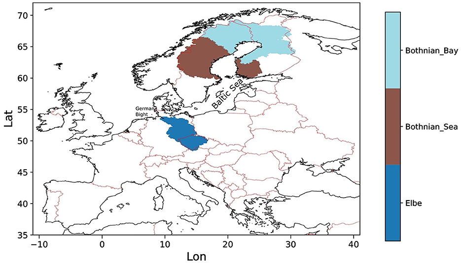
Figure 1. This image displays the seas, catchments, and regions that are mentioned by name in this study. The first two entries in the colorbar are catchment areas of rivers that discharge into the Bothnian Bay and Bothnian Sea. The last entry is the catchment area of the river Elbe.
In order to generate high-resolution water level data, hourly data of near-surface (10 meter height) wind components and sea level pressure are required (see Section 2.3). At the time of the study, only two data sets from the EURO–CORDEX archive were available to us that fulfilled this requirement. Both data sets comprise historical simulations from 1950–2005, and two scenarios following the Representative Concentration Pathways RCP 2.6 and 8.5 (Van Vuuren et al., 2011a), which span from 2005 until the end of the 21st century. The historical simulations are not based on reanalysis and can be only compared in a statistical sense.
We used two available atmospheric data sets, REMO–MPI and REMO–Had (see below), originating from two different GCMs that were dynamically downscaled to the EURO–CORDEX 0.11° domain with two different versions of the RCM REMO (Jacob et al., 2007). REMO is a three-dimensional, hydrostatic, atmospheric circulation model within a limited area, which is hosted at the Climate Service Center Germany (GERICS). The forcing data from the global simulations are prescribed at the lateral boundaries of the European domain with an exponential decrease toward the center of the model domain. The main direct influence of the boundary data lies in the eight outer grid boxes using a relaxation scheme according to Davies (1976). Both REMO versions used 27 hybrid sigma-pressure levels, which follow the surface orography in the lower levels but are independent from it at higher atmospheric model levels.
In REMO–MPI, the global climate simulations were conducted with MPI–ESM, the Earth System Model (ESM) of the Max Planck Institute for Meteorology (Giorgetta et al., 2013). The MPI–ESM consists of coupled general circulation models for the atmosphere and the ocean, and their subsystem models for land and vegetation and for the marine biogeochemistry, respectively. For the atmosphere, the LR configuration was used with a T63 (~1.9°) horizontal resolution and 47 hybrid sigma—pressure levels, while the ocean utilized a bipolar grid with 1.5° resolution (near the equator) and 40 z-levels. The two RCP scenario simulations cover actual years for the period 2005–2099. The MPI–ESM simulations were downscaled with REMO2009 (Jacob et al., 2012).
REMO–Had has utilized global climate simulations that were conducted with HadGEM2–ES, the ESM of the UK Met Office Hadley Centre (Jones et al., 2011). HadGEM2–ES is a coupled atmosphere–ocean GCM that also represents interactive land and ocean carbon cycles as well as dynamic vegetation. It was setup with an atmospheric resolution of N96 (1.875° × 1.25°) and 38 vertical levels and an ocean resolution of 1° (increasing to 1/3° at the equator) and 40 vertical levels. HadGEM2–ES simulations are run with 30-day months and the two RCP scenario simulations cover the period 2005–2099. The HadGEM2–ES simulations were downscaled with REMO2015 (Remedio et al., 2019).
River runoff was simulated with the hydrological discharge (HD) model (Hagemann et al., 2020) covering the entire European catchment region. The HD model v. 5.0 (Hagemann and Ho-Hagemann, 2021) was set up over the European domain covering the land areas between –11° W to 69° E and 27° N to 72° N with a spatial grid resolution of 5′ (ca. 8–9 km). The HD model separates the lateral water flow into the three flow processes of overland flow, baseflow, and riverflow. Overland flow and baseflow represent the fast and slow lateral flow processes within a grid box, while riverflow represents the lateral flow between grid boxes. The HD model requires gridded fields of surface and subsurface runoff (drainage) as input for overland flow and baseflow, respectively, with a temporal resolution of one day or higher. These input fields of surface runoff and drainage were taken from the REMO simulations and interpolated to the HD model grid to simulate daily discharges.
Coastal water levels are the result of an interplay of different factors that are considered in different ways. Strong onshore winds that push water masses toward the coast cause a rise of the sea surface that is commonly referred to as a storm surge. When storm surges coincide and interact with high tides the resulting water level is often referred to as storm-tide level. When mean sea level rises, this will further increase storm tide levels. In the following, we refer to storm tide levels including the effects of mean sea level rise as total water levels.
Daily tide-surge levels were obtained from tide-surge simulations with the Tidal Residual and Intertidal Mudflat Model (TRIM). In particular, a 2D version of TRIM–NP (Kapitza, 2008) was used which is a nested hydrostatic shelf sea model with spatial resolutions increasing from 12.8 km × 12.8 km in the North Atlantic to 1.6 km × 1.6 km in the German Bight. Zonal and meridional wind components at 10-meter height and sea level pressure from the REMO–MPI and REMO–Had simulations were used as hourly atmospheric forcing fields to derive tide-surge levels in the German Bight. To include tides, data from the FES2004 atlas (Lyard et al., 2006) were used at the lateral boundaries.
In order to evaluate compound flood events during the historical period (see Section 4.1), we utilized two long-term reconstructions for discharge and three tide-surge data sets. The two daily discharge data sets are based on consistent long-term reconstructions by the global hydrology model HydroPy (Stacke and Hagemann, 2021) and the hydrological discharge (HD) model (Hagemann et al., 2020). To generate these data sets, both models were forced with the ERA5 reanalysis (Hersbach et al., 2020) of the European Centre for Medium-range Weather Forecasts (ECMWF) for the time period 1979—2018 and E-OBS data (Cornes et al., 2018) for 1950—2019. Both discharge data sets cover the same European domain as described in Section 2.2. The data sets were published as Hagemann and Stacke (2021), and their generation and evaluation is described in Hagemann and Stacke (2022).
The three tide-surge reconstructions were generated by two different shelf sea models. In the first two reconstructions, the TRIM model was forced with the high-resolution regional re-analysis COSMO—REA6 of the German Weather Service (DWD) for the period 1995—2018 (Bollmeyer et al., 2015). In the second and third reconstruction, COSMO—REA6 data and data from the regional climate reconstruction coastDat3 (Petrik and Geyer, 2021) were used to force the physical part of the marine ECOSystem MOdel (ECOSMO) (Schrum and Backhaus, 1999; Daewel and Schrum, 2013) for the period of 1948—2019 (Bundesamt für Seeschifffahrt und Hydrographie, 2022).
Further information on the models, reconstructions and their evaluation are available for the HD5–ERA5 and HD5–E-OBS data in Hagemann and Stacke (2022), for ECOSMO–coastDat3 in Bundesamt für Seeschifffahrt und Hydrographie (2022), as well as for TRIM in Gaslikova et al. (2013) and Weisse et al. (2015).
While changing tide-surge levels are primarily a result of changing wind climatology, changes in total coastal water levels are result of both, changing tide-surge levels and rising mean sea levels. While changes in tide-surge levels can be obtained from the described model simulations, rising mean sea levels remain unaccounted for. In a first approximation, both effects may be added linearly (Sterl et al., 2009; Howard et al., 2010) although some errors will be introduced in shallow waters caused by the modification of tide-surges through rising mean sea level (Arns et al., 2015). Non-linear effects are typically in the order of a few centimeters for sea level rises up to 5 m (Howard et al., 2010) which can still be considered small compared to uncertainties from other neglected effects such as changing bathymetry (Benninghoff and Winter, 2019).
While for tide-surge and discharge simulations we used atmospheric forcing for the two RCP scenarios of IPCC AR5, we were unaware of regionalized sea level projections for those scenarios. We, therefore, used 50th percentiles of corresponding regionalized projections from the IPCC AR6 (Fox-Kemper et al., 2021; Garner et al., 2021a,b) for the Shared Socioeconomic Pathways (SSP) scenarios SSP1-2.6 and SSP5-8.5 (see Figure 2). The SSP scenarios approximately corresponds to the RCP scenarios with the same label (Meinshausen et al., 2020). Given that the ranges of projections by 2,100 are in the order of several decimeters, the error introduced by this approach is probably small. Relative regional sea level was used so that vertical land movements are accounted for. The latter is particularly important in the Baltic Sea where ongoing glacial isostatic adjustment (GIA) is large (Weisse et al., 2021). The region around the Gulf of Bothnia experiences a relative sea level fall, contrary to the rest of Europe. To obtain estimates of total coastal water levels the 50th percentiles derived from these projections were linearly added to the corresponding tide-surges obtained from the model simulations.
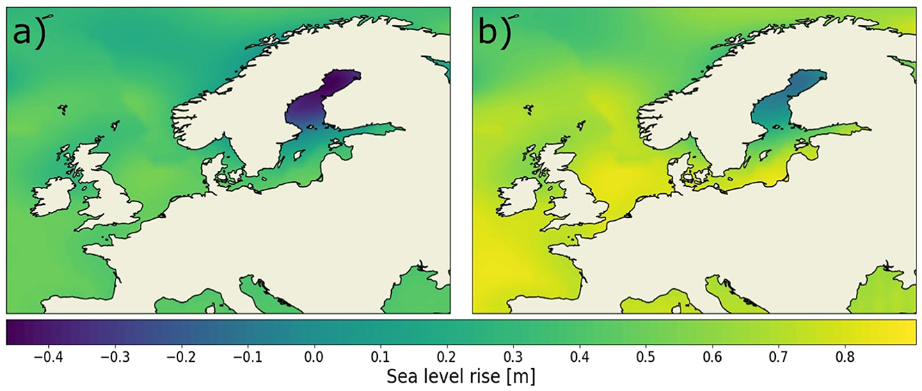
Figure 2. Projected relative sea level rise by 2099 in Europe for the 50th percentile (a) SSP1-2.6 and (b) SSP5-8.5 based on medium confidence scenario (Garner et al., 2021a).
There are several ways to identify extreme events, with no standardized method being used in published research. The goal is always to manage the trade-off between finding a low number of extremes because they are rare per definition, while at the same time having enough data points for statistical analysis. Two commonly used methods are block maxima (for example, in Moftakhari et al., 2017) and Peaks over Threshold (POT) (for example, in Fang et al., 2021), both having their upsides and downsides which were discussed in studies like Jaruskova and Hanek (2006) or Ward et al. (2018). Here, we chose Peaks over Threshold and followed a percentile-based approach for each river individually since we otherwise might miss out on events if, for example, two extreme events occur in one year. For both the water level and discharge data sets, we started at the 90th percentile. We then continued to raise the percentile in small incremental steps until the resulting thresholds for each river yielded on average two extreme events per year. This was done for the historical runs, with the same thresholds being used for future scenarios unless stated otherwise. To ensure that extreme events identified that way are independent of each other we additionally applied a de-clustering algorithm that guaranteed that different extreme events are separated by at least 3 days. Due to the scale of the study domain it is not feasible to employ a site specific de-clustering time for each individual river. Therefore, we chose a time that was used by previous large scale studies like Ward et al. (2018) and Bevacqua et al. (2019). In other words, all events that are less than four days apart from each other are considered to belong to the same extreme event. An event was counted as a compound event when an extreme discharge and extreme coastal water level event occurred on the same day. Some studies use temporal delay (lag) to account for the delays between variables reacting to an event. Ganguli and Merz (2019) calculated the lag based on the catchment area, but for long rivers like the Elbe the actual delay heavily depends on the location of the occurring precipitation. We did not utilize lag so that we only detect events where the variables are extreme at the same time.
We utilized a Monte Carlo approach to identify those rivers in which compound flood occurred more frequently than expected for uncorrelated drivers. Compound flood events in rivers that show a higher number of compound flood events than expected by chance might have a common driver. For this analysis we limited the data sets to the winter seasons, since this is where storm surges mostly occur in northern Europe (Liu et al., 2022). To remove possible correlations between the data sets we shuffled the tide-surge data. This creates a data set where discharge and tide-surge data are independent. Afterwards, we counted the number of compound flood events for the combination of discharge and randomized coastal water level data to see how it changed compared to a data set with possible dependence between extreme events. The process was repeated 10,000 times to create a probability distribution for uncorrelated events for each river. This allowed us to assess whether or not the observed distribution is outside the 95% range (2σ) of the distributions for independent drivers which provides an indication for correlated drivers. A more detailed analysis, including the reasoning for our choices, is given in Heinrich et al. (2023).
We calculated the duration of each season in order to analyze changes in the seasonality of compound flood events. The duration of a season was defined as the shortest time period that contains at least 90% of the compound flood event days, similar to the definition by Bevacqua et al. (2020). For this, we first counted the number of compound flood event days per month in the time period of the data set, e.g., the number of days that occur each March throughout the entire time period that we analyzed. We accumulated the number of days instead of the number of compound flood events to take into account that the length of compound flood events might change in the future, so simply counting the number might underestimate the differences. Furthermore, this approach takes into consideration that a compound flood event might start at the end of a month and continue into the next month. Then we used the NumPy sliding window view function (Harris et al., 2020) to find the shortest combination of months that contained at least 90% of the accumulated compound flood event days. If there was a month without compound flood event days in a season, it was counted as part of it for the sake of continuity.
The intensity of extreme discharge events was defined as the average amount of discharge during an extreme event. This means that the intensity is based on the total discharge during this event. These calculations were also done for coastal water levels, where the intensity is the total water height during the extreme event.
To disentangle the contributions of the different drivers to future changes in compound flood event frequency, we set up different data set combinations (Table 1). As shown in Section 4.4, tide-surges do not show any significant changes under RCP2.6 and RCP8.5 scenarios, as long as sea level rise is neglected. For the analysis it was important to not distort correlations between extreme events of discharge and coastal water levels because this would influence the number of compound flood event days (Heinrich et al., 2023). To have a reference, we calculated the number of compound flood event days in both REMO data sets for the historical time period 1976–2005. To test the contribution of discharge to frequency changes in future compound flood events, we used discharge and tide-surge from the future time period 2070–2099 since the historical and future tide-surge levels are nearly identical. Afterwards, we evaluated the contribution of sea level rise by adding it to the tide-surge levels of the historical data sets. This again preserves possible correlations.
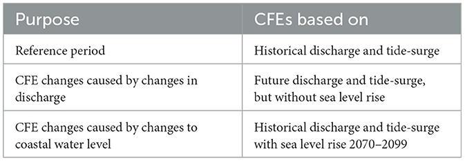
Table 1. Purpose of data sets to analyze the contribution of discharge and sea level rise to future compound flood event frequency.
In the following sections we first evaluate the historical runs of our data sets, then investigate the changes of the separate drivers before proceeding to look into future changes to compound flood events.
Figure 3 shows a comparison between the historical runs of the REMO downscaled global climate models and the reconstruction data HD5–ERA5+TRIM–REA6 for the number of compound flood events over a time period of 24 years. Generally, the REMO data sets show a similar number of compound flood events (Figures 3a, c, e). Only for the northern coast of Norway and occasionally rivers near the Baltic States a systematic overestimation is obtained. Using the Monte Carlo approach (see Section 3.2), we estimated which rivers show a larger number of compounds than could be expected from uncorrelated drivers. The reconstruction data set of HD5–ERA5+TRIM–REA6 shows a larger number of rivers along the western-facing coasts having a higher number of compound flood events than could be expected by random coincidence of uncorrelated extremes (Figures 3a, b). A comparable pattern could also be identified in the REMO data sets, even though it is less pronounced (Figures 3d, f). A comparison of the REMO data sets with HD5–E-OBS+ECOSMO–coastDat3 and HD5–ERA5+ECOSMO–coastDat3 over a time period of 30 years shows again a slight overestimation like the TRIM-based data sets (Supplementary Figure S3). No information is available on potential deviations in Norway and parts of western Europe like Ireland, because ECOSMO–coastDat3 covers a smaller domain. As in the reconstruction data sets, the compound flood events in the REMO data sets are mostly limited to the period of November to March.
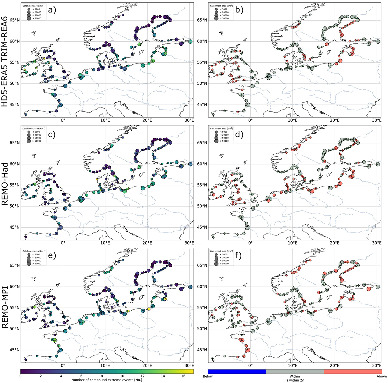
Figure 3. Number of compound flood events (left) and dependence/independence between drivers (right) in the HD5–ERA5+TRIM–REA6 reconstruction (top), the REMO–Had (middle) and the REMO–MPI (bottom) historical runs. Colors indicate the number of compound events over 24 years and whether or not this number is within (gray), above (red) or below (blue) the expected 2σ interval derived from randomized Monte Carlo simulations. The size of the circles indicates the catchment area.
We investigated changes in the frequency and intensity of discharge extreme events for the two scenarios. Discharge intensity increases for most catchments in Ireland and Great Britain under the RCP 2.6 scenario while it decreases for most of the rivers discharging into the Baltic Sea (Figures 4a, c). Similar changes can be observed for the number of extreme discharge days (Figures 5a, c). Slight disagreements arise between the data sets for central Europe. REMO–MPI projects a decrease in intensity at the western coast of the Bothnian Bay, Great Britain, and the north-facing coasts of France, Germany, and Poland, while REMO–Had projects an increase under RCP2.6 for those regions. For the regions with disagreement, the projected changes are rather minor. Despite that, REMO–Had and REMO–MPI mostly agree in their assessment that the northern coasts of Poland and Germany will have a lower number of extreme event days.
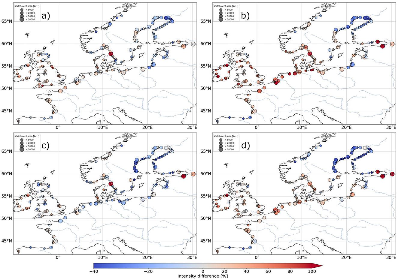
Figure 4. Changes in discharge intensity toward the end of the century (2070–2099) relative to the historical reference period (1976–2005). (a) REMO–Had RCP2.6, (b) REMO–Had RCP8.5, (c) REMO–MPI RCP2.6, (d) REMO–MPI RCP8.5.
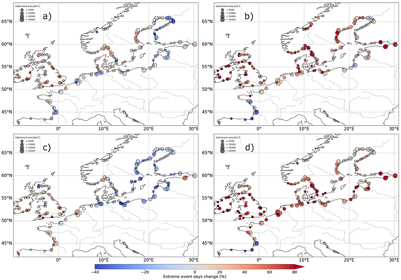
Figure 5. Changes in the total number of days with extreme discharge toward the end of the century (2070–2099) relative to the historical reference period (1976–2005). (a) REMO–Had RCP2.6, (b) REMO–Had RCP8.5, (c) REMO–MPI RCP2.6, (d) REMO–MPI RCP8.5. The percentages are calculated as changes to the number of days with extreme discharge in the historical period.
The REMO data sets show a stronger agreement for intensity and number of extreme days changes under RCP8.5, with most of Europe experiencing an increase for both parameters (Figures 4b, d, 5b, d). A lower intensity is anticipated by both REMO data sets only for northern Spain and the Bothnian Bay. The number of days with extreme discharge increases throughout all of Europe, with the exception of northern Spain. As in RCP 2.6, the REMO data sets disagree for the northern Norwegian coast and the western coast in the Bothnian Sea. The increases and decreases of both variables are much stronger than under RCP2.6.
The tide-surge component of the total coastal water level shows no significant change in both RCP scenarios; that is if sea level rise is neglected. Figure 6 exemplifies this for the coastal water levels at the Elbe river mouth. Both tide-surge data sets show very similar distributions in the histogram. The same behavior can be seen for all other rivers. As a result, the intensity and number of the extreme tide-surge events does stays similar.
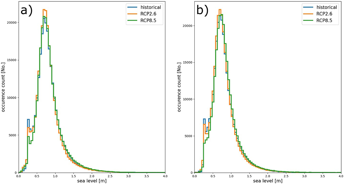
Figure 6. Histogram containing hourly tide-surge level values for (a) REMO–Had and (b) REMO–MPI as calculated by the TRIM model at the Elbe river mouth. The histogram is based on 100 bins with sea level rise being neglected. The historical time period is 1976–2005, while future scenarios RCP2.6 and RCP8.5 cover the years 2070–2099.
The number of compound flood event days at the end of the century shows large local differences (Figure 7). While nearly all of Europe experiences an increase in the number of compound flood events in RCP2.6 and RCP8.5, this is not the case for the Bothnian Bay and Bothnian Sea. There we see mostly similar amounts of compound flood event days under RCP2.6 at the end of the current century, with some rivers even indicating a decrease. The reason for this is that this regions already has a low number of compound flood event days in the historical reference period and in the RCP scenarios, discharge slightly increases while the sea level lowers at the same time. For RCP8.5, the increase of compound flood event days for this region is weaker compared to the rest of Europe. This is because the sea level is similar to the historical one, while there is an increase in discharge event days.
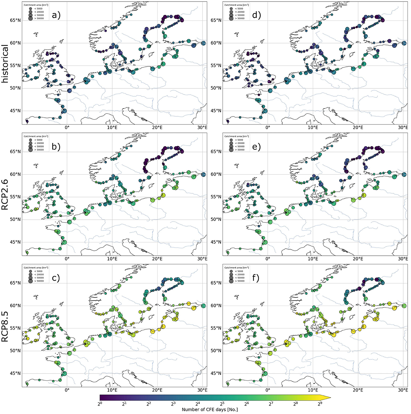
Figure 7. Number of compound flood event days in Europe over a period of 30 years on a logarithmic scale. The historical reference period covers 1976–2005, while the future scenarios cover 2070–2099. The left column shows the REMO–Had scenarios (a) historic, (b) RCP2.6, and (c) RCP8.5. In the same way, the right column shows REMO–MPI for (d) historical scenario, (e) RCP2.6, and (f) RCP8.5.
The mean duration of the compound flood event season in all rivers elongates in both REMO data sets for the future scenarios (Table 2). For RCP2.6, REMO–Had and REMO–MPI project an increase of around 0.8 and 0.3 months respectively. For RCP8.5 the compound flood event season is even longer by around 1.6 and 1.1 months in comparison to the historical reference period. This increase can be attributed to the rising sea level extending the duration of the storm surge season and therefore creating a bigger overlap with the discharge season.
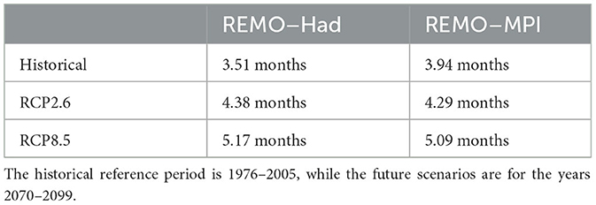
Table 2. Average compound flood event season duration calculated over all rivers that are considered in this study.
In the historical period (Figure 8) western-facing coasts have a higher chance of showing more compound flood events than expected by chance. If the chosen thresholds are adapted to the future scenarios (see Section 3.1), a similar pattern can be inferred. If thresholds are not adapted to future changes, however, nearly all rivers will have a number of compound flood events that is above the expected 2σ value of the historical reference period. The only exception to this are the rivers in the Bothnian Bay and Bothnian Sea.
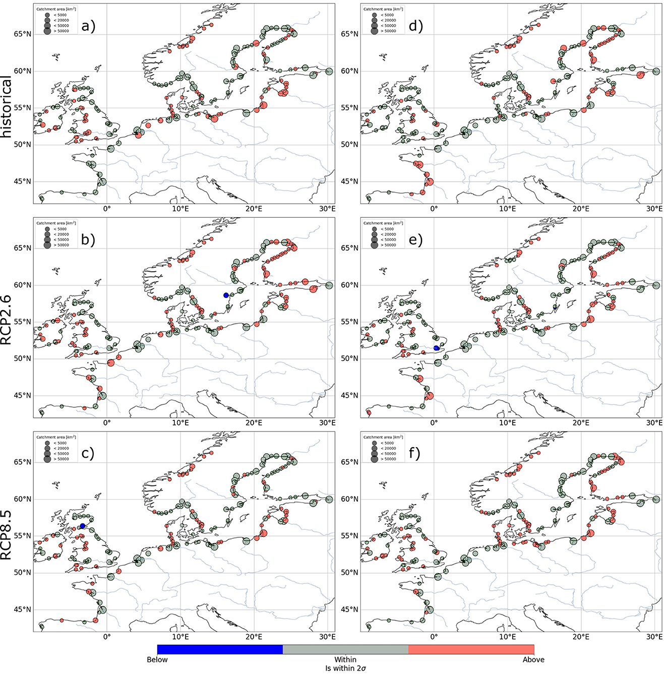
Figure 8. Comparison of dependence/independence between drivers for rivers in northern Europe for the historical reference period (1976–2005) and the end of the century (2070–2099), with each using thresholds that were newly calculated for the corresponding time period. The color of the circles displays if the amount of compound flood events is within (gray), above (red), or below (blue) the expected 2σ interval interval derived from randomized Monte Carlo simulations. (Left) column contains REMO–Had data and the (right) one REMO–MPI. The rows contain historical reference (top), RCP2.6 scenario (middle), and RCP8.5 scenario (bottom).
How much future changes in discharge and sea level rise contribute to changes in the number of compound flood event days, can be seen for RCP2.6 in Figure 9 and for RCP8.5 in Figure 10. It shows that sea level rise is the main contributor to the observed changes in compound flood events. Nevertheless, future changes in discharge will add to those changes, tide-surge share in it is negligible.
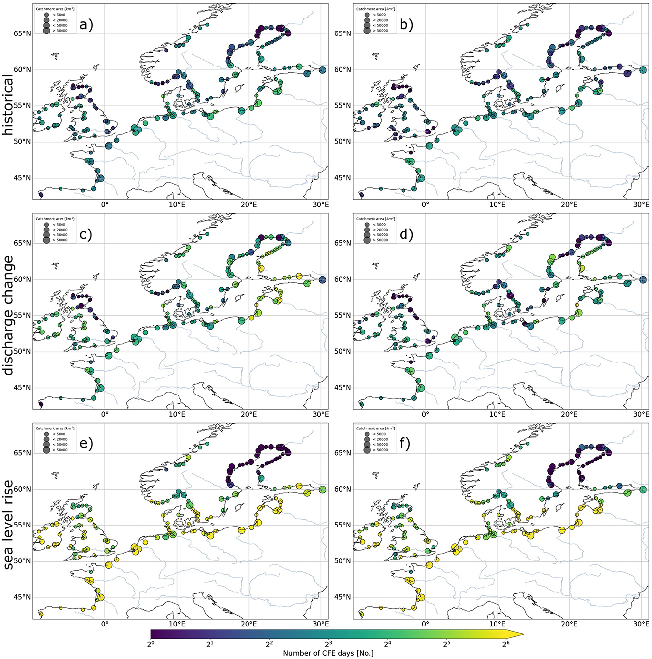
Figure 9. Contribution of discharge and sea level rise to changes in the total number of compound flood event days under RCP2.6. The (left column) contains changes for REMO–Had, (right column) for REMO–MPI. The top row contains the number of compound flood events of the historical runs. The middle row utilized discharge and tide-surge level (without sea level rise) of the time period 2070–2099 to calculate the compound flood events. The bottom row used the discharge and total coastal water level (tide-surge plus mean sea level) from the historical time period but added the sea level rise that corresponds to 2070–2099. An explanation for those choices is given in Section 3.5.
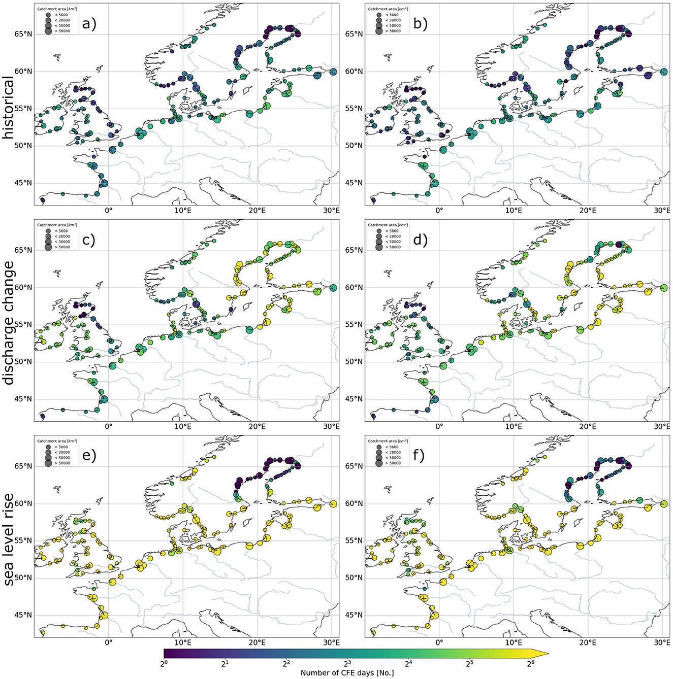
Figure 10. Contribution of discharge and sea level rise to changes in the total number of compound flood event days under RCP8.5. The (left column) contains changes for REMO–Had, (right column) for REMO–MPI. The top row contains the number of compound flood events of the historical runs. The middle row utilized discharge and coastal water level (without sea level rise) of the time period 2070–2099 to calculate the compound flood events. The bottom row used the discharge and total coastal water level (tide-surge plus mean sea level) from the historical time period but added the sea level rise that corresponds to 2070–2099. An explanation for those choices is given in Section 3.5.
Comparing the historical runs of the REMO data sets with the reconstruction data (Section 4.1) showed a very similar behavior. Both REMO data sets show a number of compound flood events that is similar to those of the reconstruction data sets, even if the compound flood events for northern Norway are overestimated. Furthermore, there is a certain amount of variability due to the events being infrequent and the analysis time period being comparably small. For both REMO data sets the majority of compound flood events happen in the winter months. Also, the 2σ maps (Figure 3), which show if a river has more compound flood events than expected by chance, show a similar pattern, with the western-facing coasts tending to be above the 2σ range. The deviations we observe are potentially caused by slightly different storm trajectories in the REMO data sets and natural climate variability which does not allow a one to one comparison since they are not based on reanalysis.
If sea level rise is neglected, we do not see changes in the coastal water levels. There are studies that project an increase in cyclone number and mean wind speed (e.g., Zappa et al., 2013) as well as a poleward shift of the storm tracks (e.g., Kjellström et al., 2018). However, those results are sensitive to the chosen forcing and the choice of the global climate model (Feser et al., 2015; Ozturk et al., 2022). Gonzalez et al. (2019) concluded that those projections should be viewed with some caution. Discharge on the other hand shows a change in the number of extreme event days and intensity. These changes in discharge are caused by an increase in global temperature. Higher temperature results in the atmosphere carrying more moisture, which eventually leads to more extreme precipitation events in most parts of northern Europe in winter (Pfahl et al., 2017). Furthermore, due to warmer winters, the snow melt will start sooner (Blöschl et al., 2017), leading to a seasonality shift in many regions like Scandinavia. Hattermann et al. (2015) found that a combination of those factors would lead to an increase in winter discharge for almost all large German rivers. This makes it important to have proper discharge data available that take snow melt into account like in the current study, instead of only precipitation. The period of strong discharge events will begin earlier in winter and therefore lasts for an extended period in comparison to the historical time frame. This, combined with more precipitation events leads to changes in the number of extreme event days. The increased annual precipitation (Rajczak and Schär, 2017) will result in a generally higher discharge level in Europe (Thober et al., 2018). An exception to this is northern Spain where we see a reduction in intensity and extreme discharge days due to less precipitation. While the signals are very clear in the REMO data sets for RCP8.5, this is not the case for RCP2.6. Like in Di Sante et al. (2021), clear changes to discharge can be seen for Scandinavia and the Baltic States, but not for most of central and western Europe. The decrease in extreme discharge event days under RCP2.6 might be caused by the warmer temperature leading to less snow melt-generated discharge. Overall, our results match the generally expected future discharge changes.
Due to sea level rise and increased discharge, we expect a strong increase in compound flood events toward the end of the century in both scenarios. The changes are significant for both RCP scenarios, but much stronger in RCP8.5. Our analysis reveals that sea level rise will be the main contributor to those changes for most of Europe (see Figures 9, 10). However, even if sea level rise is ignored, the changes in discharge under RCP8.5 are large enough to cause major shifts in compound flood event frequency. Despite that, it is essential to take into account, that changes in discharge event frequency and intensity will have impacts on a local scale. The developments of sea level rise and discharge will furthermore cause an increase in the compound flood event season duration which is projected to extend up to 5 months under RCP8.5 at the end of the current century. Furthermore, we see that by adapting the thresholds to future scenarios, the pattern in Figure 8 remains similar, indicating that the generating mechanism for most compound flood events stays the same. If those thresholds are not adapted and stay on the historical level, nearly all rivers show more events than in the past. Our results, therefore, align with the work of Bevacqua et al. (2019) who projected a rise in compound flood events toward the end of the century. Our results do not find any indication of a widespread lower risk of compound flood events over central Europe as described by Ganguli et al. (2020). One reason for the difference in results might be that their study investigated the middle of the century (2040—2069), while the climate change signals increases in magnitude throughout the century. It also must be noted that ourapproach to classify compound flood events is different to the one used by Ganguli et al. (2020). The present study utilizes a Peaks over Threshold approach, while the former uses annual maxima high coastal water levels and high river discharge within ±7-days of occurrence of the high coastal water level.
As discussed, sea level rise is the dominant factor responsible for future changes in compound flood events. To assess how sea level rise may affect the number of compound events for different global warming levels, we added the corresponding sea level rise to the historical tide-surge data sets and left the discharge unchanged. As shown in Figure 2, the Bothnian Bay and Bothnian Sea do not experience sea level rise and will therefore not be explicitly named every time in the following as an exception to the general trends. A sea level rise associated with a 1.5K global warming already rises the number of compound flood event days strongly. Here, SSP1-2.6 (Figure 11) and SSP5-8.5 (Figure 12a) will double the amount of compound flood event days for southern England, eastern coast of Great Britain, Ireland, and the Western Baltic. Nearly all European rivers will experience an increase of 50% or more, with the exception of northern Norway. With global temperature rise crossing a warming of 2K all of Europe would experience twice the number of compound flood events compared to the historical reference period (Figure 12b), except for northern Norway and the northwestern German coast. In a similar fashion, a 3K temperature increase would triple the numbers of compound flood event days (Figure 12c) and 4K would raise it by a factor of 5 (Figure 12d). This demonstrates, that even if the global warming will be limited to 2K or less, the resulting sea level rise will impose a massively increased risk on the European countries.
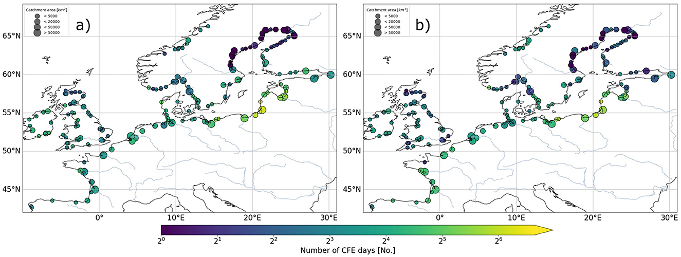
Figure 11. Number of compound flood event days over 30 years if the sea level rise, which is associated with a specific level of global warming in SSP1-2.6, had occurred in the historical time period (1976–2005). (a) shows those changes for REMO–Had and (b) for REMO–MPI. The global average temperature increase is 1.5K. The point at which the temperature increase is reached can be seen in Supplementary Table S3.
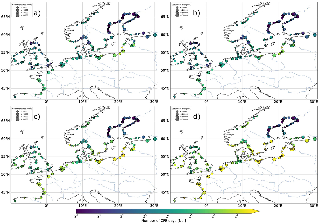
Figure 12. Number of compound flood event days over 30 years if the sea level rise, which is associated with a specific level of global warming in SSP5-8.5, had occurred in the historical time period (1976–2005). This image shows REMO–MPI. The very similar figure for REMO–Had (Supplementary Figure S2) can be seen in the supplementary material. The temperature increase is 1.5K in (a), 2K in (b), 3K in (c), and 4K in (d). The point at which the temperature increase is reached can be seen in Supplementary Table S3.
It should also be taken into account that the number of annual compound flood events underlies natural variability. This can be seen in the variations of the 5 year average (Figure 13). A clear separation between RCP2.6 and RCP8.5 starts to emerge around the 2060s for both REMO data sets. The climate signal strength and amount of changes depend on the forcing and the time period, with most changes happening in the second half of the century. Nevertheless, a generally rising trend can be seen for the entire time period.
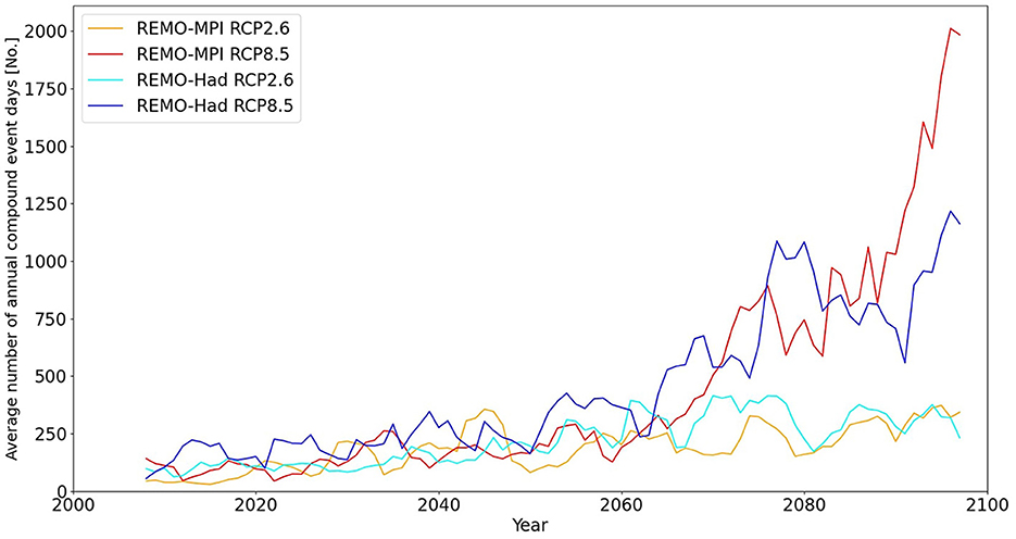
Figure 13. Sum of annual compound flood event days over a 5 year moving average for all rivers combined in the study area from 2006 to 2099. The calculation of compound flood events includes local changes to the coastal water levels caused by sea level rise.
A large-scale study like this comes with inevitable caveats. Only data sets from two downscaled different global models were available due to the required high temporal resolution for the TRIM simulation. Due to not having an ensemble of available data sets we yielded uncertain changes in the discharge under RCP2.6 for parts of Europe. This goes hand in hand with compound flood events being a phenomenon that underlies large variability as seen in Figure 13. Therefore, even 30-year time frames have a certain amount of variability, especially with the ongoing influence of climate change. Furthermore, the evaluation of the model performance showed that the general patterns can be represented, but differences exist nonetheless due to limitations in the modeling frameworks. Additionally, the uncertain absolute amount of sea level rise, as well as the linear superposition of tides with sea level rise, adds a noticeable uncertainty to the question of how strong the changes in future extreme events will be since it is the predominant factor. Note that due to the large scale of the domain of our study, it was not possible to take local factors like flood protection and topography into account.
In the present study, we conducted an analysis of future changes in compound flood events over northern and central Europe and the contributing factors to it without the use of copulas. We have demonstrated that the number of compound flood events will strongly increase in the future, regardless of the scenario. Furthermore, we analyzed future changes in discharge and coastal water levels. To the authors' knowledge, this is the first study that investigates these changes without the use of copulas in Europe. It is important to point out that this study should be seen as a general trend analysis for future scenarios and not as an actual prediction that can be used for precise flood risk assessment. Scenario RCP2.6 shows a less extreme increase in compound flood events compared to RCP8.5. The main contributor to those changes is sea level rise, while changes in river discharge are less severe but are not negligible. The sea level rise will lead to a strong increase in compound flood events, even when the global warming is limited in line with the Paris Agreement. The magnitude of those changes increases toward the end of the current century. In general, REMO–Had and REMO–MPI show strong agreement for RCP8.5, but less for RCP2.6. Additionally, we see in a future with adjusted thresholds that west-facing coasts experiencing a higher number of flood events than expected by pure chance, just like in the historical reference period. This implies that the strongest compound flood events in future scenarios will still be caused by a common driver like a specific weather constellation. Future work can further examine climate change under RCP2.6 and RCP8.5 by utilizing an ensemble of global climate models. This, paired with a better understanding of sea level rise on a local level, will be important to lower the uncertainty in changes to future compound flood events, which is essential for accurate risk assessment.
The original contributions presented in the study are included in the article/Supplementary material, further inquiries can be directed to the corresponding author.
PH developed the analysis methods, performed the data analysis, and wrote the manuscript. SH initiated the study and contributed the HD discharge data while LG generated the TRIM data. RW and SH supervised the research activities, revised the manuscript, and contributed to the interpretation of the results. RW acquired the funding. All authors contributed to the article and approved the submitted version.
This research was financed with funding provided by the German Federal Ministry of Education and Research (BMBF; Förderkennzeichen 01LR2003A).
This research is a contribution to the PoFIV program of the Helmholtz Association. We thank the projection authors for developing and making the sea-level rise projections available, multiple funding agencies for supporting the development of the projections, and the NASA Sea Level Change Team for developing and hosting the IPCC AR6 Sea Level Projection Tool.
The authors declare that the research was conducted in the absence of any commercial or financial relationships that could be construed as a potential conflict of interest.
All claims expressed in this article are solely those of the authors and do not necessarily represent those of their affiliated organizations, or those of the publisher, the editors and the reviewers. Any product that may be evaluated in this article, or claim that may be made by its manufacturer, is not guaranteed or endorsed by the publisher.
The Supplementary Material for this article can be found online at: https://www.frontiersin.org/articles/10.3389/fclim.2023.1227613/full#supplementary-material
Arns, A., Wahl, T., Dangendorf, S., and Jensen, J. (2015). The impact of sea level rise on storm surge water levels in the northern part of the german bight. Coastal Eng. 96, 118–131. doi: 10.1016/j.coastaleng.2014.12.002
Benninghoff, M., and Winter, C. (2019). Recent morphologic evolution of the german wadden sea. Scient. Rep. 9, 1–9. doi: 10.1038/s41598-019-45683-1
Bermúdez, M., Farfán, J., Willems, P., and Cea, L. (2021). Assessing the effects of climate change on compound flooding in coastal river areas. Water Resour. Res. 57, e2020WR029321. doi: 10.1029/2020WR029321
Bevacqua, E., Maraun, D., Vousdoukas, M. I., Voukouvalas, E., Vrac, M., Mentaschi, L., et al. (2019). Higher probability of compound flooding from precipitation and storm surge in europe under anthropogenic climate change. Sci. Adv. 5, eaaw5531. doi: 10.1126/sciadv.aaw5531
Bevacqua, E., Vousdoukas, M. I., Zappa, G., Hodges, K., Shepherd, T. G., Maraun, D., et al. (2020). More meteorological events that drive compound coastal flooding are projected under climate change. Commun. Earth Environ. 1, 1–11. doi: 10.1038/s43247-020-00044-z
Blöschl, G., Hall, J., Parajka, J., Perdigão, R. A. P., Merz, B., Arheimer, B., et al. (2017). Changing climate shifts timing of european floods. Science 357, 588–590. doi: 10.1126/science.aan2506
Bollmeyer, C., Keller, J., Ohlwein, C., Wahl, S., Crewell, S., Friederichs, P., et al. (2015). Towards a high-resolution regional reanalysis for the european cordex domain. Quart. J. R. Meteorol. Soc. 141, 1–15. doi: 10.1002/qj.2486
Bundesamt für Seeschifffahrt und Hydrographie (2022). Report on the oceanographic conditions at site n-7.2. Available online at: https://www.bsh.de/EN/TOPICS/Offshore/Offshore_site_investigations/Procedure/N-07-02/N-07-02_node.html (accessed April 19, 2022).
Cornes, R. C., van der Schrier, G., van den Besselaar, E. J., and Jones, P. D. (2018). An ensemble version of the e-obs temperature and precipitation data sets. J. Geophys. Res. 123, 9391–9409. doi: 10.1029/2017JD028200
Couasnon, A., Eilander, D., Muis, S., Veldkamp, T. I., Haigh, I. D., Wahl, T., et al. (2020). Measuring compound flood potential from river discharge and storm surge extremes at the global scale. Nat. Haz. Earth Syst. Sci. 20, 489–504. doi: 10.5194/nhess-20-489-2020
Daewel, U., and Schrum, C. (2013). Simulating long-term dynamics of the coupled north sea and baltic sea ecosystem with ecosmo ii: Model description and validation. J. Mar. Syst. 119, 30–49. doi: 10.1016/j.jmarsys.2013.03.008
Davies, H. (1976). A lateral boundary formulation for multi-level prediction models. Quart. J. R. Meteorol. Soc. 102, 405–418. doi: 10.1002/qj.49710243210
Di Sante, F., Coppola, E., and Giorgi, F. (2021). Projections of river floods in europe using euro-cordex, cmip5 and cmip6 simulations. Int. J. Climatol. 41, 3203–3221. doi: 10.1002/joc.7014
Douben, K.-J. (2006). Characteristics of river floods and flooding: a global overview, 1985-2003. Irrigat. Drain. 55, S9S21. doi: 10.1002/ird.239
Fang, J., Wahl, T., Fang, J., Sun, X., Kong, F., and Liu, M. (2021). Compound flood potential from storm surge and heavy precipitation in coastal china: dependence, drivers, and impacts. Hydrol. Earth Syst. Sci. 25, 4403–4416. doi: 10.5194/hess-25-4403-2021
Feser, F., Barcikowska, M., Krueger, O., Schenk, F., Weisse, R., and Xia, L. (2015). Storminess over the north atlantic and northwestern europea review. Quart. J. R. Meteorol. Soc. 141, 350–382. doi: 10.1002/qj.2364
Feyen, L., Ciscar Martinez, J. C., Gosling, S., Ibarreta Ruiz, D., and Soria Ramirez, A. (2020). Climate change impacts and adaptation in Europe JRC peseta IV final report. Technical report, Joint Research Centre (Seville site).
Fox-Kemper, B., Hewitt, H., Xiao, C., Adalgeirsdottir, G., Drijfhout, S., Edwards, T., et al. (2021). Ocean, Cryosphere and Sea Level Change, book section 9. Cambridge, United Kingdom and New York, NY, USA: Cambridge University Press 1211–1362.
Ganguli, P., and Merz, B. (2019). Trends in compound flooding in northwestern europe during 1901-2014. Geophys. Res. Lett. 46, 10810–10820. doi: 10.1029/2019GL084220
Ganguli, P., Paprotny, D., Hasan, M., Güntner, A., and Merz, B. (2020). Projected changes in compound flood hazard from riverine and coastal floods in northwestern europe. Earth's Fut. 8, e2020EF001752. doi: 10.1029/2020EF001752
Garner, G., Hermans, T., Kopp, R., Slangen, A., Edwards, T., Levermann, A., et al. (2021a). IPCC AR6 sea level projections. Version 20210809. Available online at: https://podaac.jpl.nasa.gov/announcements/2021-08-09-Sea-level-projections-from-the-IPCC-6th-Assessment-Report (accessed July 12, 2022).
Garner, G., Kopp, R., Hermans, T., Slangen, A., Koubbe, G., Turilli, M., et al. (2021b). Framework for assessing changes to sea-level (facts), IPCC AR6 sea-level rise projections, version 20210809, in Preparation Framework for Assessing Changes To Sea-level (FACTS) (Geoscientific Model Development).
Gaslikova, L., Grabemann, I., and Groll, N. (2013). Changes in north sea storm surge conditions for four transient future climate realizations. Nat. Haz. 66, 1501–1518. doi: 10.1007/s11069-012-0279-1
Giorgetta, M. A., Jungclaus, J., Reick, C. H., Legutke, S., Bader, J., Böttinger, M., et al. (2013). Climate and carbon cycle changes from 1850 to 2100 in mpi-esm simulations for the coupled model intercomparison project phase 5. J. Adv. Model. Earth Syst. 5, 572–597. doi: 10.1002/jame.20038
Giorgi, F., Jones, C., and Asrar, G. R. (2009). Addressing climate information needs at the regional level: the cordex framework. World Meteorol. Organiz. Bull. 58, 175.
Gonzalez, P. L., Brayshaw, D. J., and Zappa, G. (2019). The contribution of north atlantic atmospheric circulation shifts to future wind speed projections for wind power over europe. Clim. Dyn. 53, 4095–4113. doi: 10.1007/s00382-019-04776-3
Hagemann, S., and Ho-Hagemann, H. T. (2021). The hydrological discharge model - a river runoff component for offline and coupled model applications. Zenodo 10. doi: 10.5281/zenodo.4893099
Hagemann, S., and Stacke, T. (2021). Forcing for HD Model from HydroPy and subsequent HD Model river runoff over Europe based on EOBS22 and ERA5 data. World Data Center for Climate (WDCC) at DKRZ.
Hagemann, S., and Stacke, T. (2022). Complementing ERA5 and E-OBS with high-resolution river discharge over Europe. Oceanologia 65, 230–248. doi: 10.1016/j.oceano.2022.07.003
Hagemann, S., Stacke, T., and Ho-Hagemann, H. (2020). High resolution discharge simulations over europe and the baltic sea catchment. Front. Earth Sci. 8, 12. doi: 10.3389/feart.2020.00012
Harris, C. R., Millman, K. J., van der Walt, S. J., Gommers, R., Virtanen, P., Cournapeau, D., et al. (2020). Array programming with NumPy. Nature 585, 357–362. doi: 10.1038/s41586-020-2649-2
Harrison, L. M., Coulthard, T. J., Robins, P. E., and Lewis, M. J. (2022). Sensitivity of estuaries to compound flooding. Estuar. Coasts 45, 1250–1269. doi: 10.1007/s12237-021-00996-1
Hattermann, F. F., Huang, S., and Koch, H. (2015). Climate change impacts on hydrology and water resources. Meteorol. Zeitschrift 24, 201–211. doi: 10.1127/metz/2014/0575
Hausfather, Z., and Peters, G. P. (2020). Emissions-the business as usual story is misleading. Nature 577, 618–620. doi: 10.1038/d41586-020-00177-3
Heinrich, P., Hagemann, S., Weisse, R., Schrum, C., Daewel, U., and Gaslikova, L. (2023). Compound flood events: analysing the joint occurrence of extreme river discharge events and storm surges in northern and central europe. Nat. Haz. Earth Syst. Sci. Disc. 23, 1967–1985. doi: 10.5194/nhess-23-1967-2023
Hendry, A., Haigh, I. D., Nicholls, R. J., Winter, H., Neal, R., Wahl, T., et al. (2019). Assessing the characteristics and drivers of compound flooding events around the uk coast. Hydrol. Earth Syst. Sci. 23, 3117–3139. doi: 10.5194/hess-23-3117-2019
Hersbach, H., Bell, B., Berrisford, P., Hirahara, S., Horányi, A., Muñoz-Sabater, J., et al. (2020). The ERA5 global reanalysis. Q. J. Royal Meterol. Soc. 146, 1999–2049. doi: 10.1002/qj.3803
Howard, T., Lowe, J., and Horsburgh, K. (2010). Interpreting century-scale changes in southern north sea storm surge climate derived from coupled model simulations. J. Clim. 23, 6234–6247. doi: 10.1175/2010JCLI3520.1
IPCC. (2021). Climate Change 2021: The Physical Science Basis. Contribution of Working Group I to the Sixth Assessment Report of the Intergovernmental Panel on Climate Change. Cambridge; New York, NY: Cambridge University Press. doi: 10.1017/9781009157896
Jacob, D., Bärring, L., Christensen, O. B., Christensen, J. H., de Castro, M., Déqué, M., et al. (2007). An inter-comparison of regional climate models for europe: model performance in present-day climate. Clim. Change 81, 31–52. doi: 10.1007/s10584-006-9213-4
Jacob, D., Elizalde, A., Haensler, A., Hagemann, S., Kumar, P., Podzun, R., et al. (2012). Assessing the transferability of the regional climate model remo to different coordinated regional climate downscaling experiment (cordex) regions. Atmosphere 3, 181–199. doi: 10.3390/atmos3010181
Jacob, D., Petersen, J., Eggert, B., Alias, A., Christensen, O. B., Bouwer, L. M., et al. (2014). Euro-cordex: new high-resolution climate change projections for european impact research. Reg. Environ. Change 14, 563–578. doi: 10.1007/s10113-013-0499-2
Jaruskova, D., and Hanek, M. (2006). Peaks over threshold method in comparison with block-maxima method for estimating high return levels of several northern moravia precipitation and discharges series. J. Hydrol. Hydromech. 54, 309–319. Available online at: http://www.uh.sav.sk/vc_articles/2006_54_4_Jaruskova_309.pdf
Jones, C. D., Hughes, J. K., Bellouin, N., Hardiman, S. C., Jones, G. S., Knight, J., et al. (2011). The hadgem2-es implementation of cmip5 centennial simulations. Geosci. Model Dev. 4, 543–570. doi: 10.5194/gmd-4-543-2011
Kapitza, H. (2008). Mops-a morphodynamical prediction system on cluster computers, in International Conference on High Performance Computing for Computational Science (Springer) 63–68. doi: 10.1007/978-3-540-92859-1_8
Kew, S., Selten, F., Lenderink, G., and Hazeleger, W. (2013). The simultaneous occurrence of surge and discharge extremes for the rhine delta. Nat. Haz. Earth Syst. Sci. 13, 2017–2029. doi: 10.5194/nhess-13-2017-2013
Kjellström, E., Nikulin, G., Strandberg, G., Christensen, O. B., Jacob, D., Keuler, K., et al. (2018). European climate change at global mean temperature increases of 1.5 and 2 c above pre-industrial conditions as simulated by the euro-cordex regional climate models. Earth Syst. Dyn. 9, 459–478. doi: 10.5194/esd-9-459-2018
Klerk, W.-J., Winsemius, H., Van Verseveld, W., Bakker, A., and Diermanse, F. (2015). The co-incidence of storm surges and extreme discharges within the rhine-meuse delta. Environ. Res. Lett. 10, 035005. doi: 10.1088/1748-9326/10/3/035005
Leonard, M., Westra, S., Phatak, A., Lambert, M., van den Hurk, B., McInnes, K., et al. (2014). A compound event framework for understanding extreme impacts. Clim. Change 5, 113–128. doi: 10.1002/wcc.252
Liu, X., Meinke, I., and Weisse, R. (2022). Still normal? Near-real-time evaluation of storm surge events in the context of climate change. Nat. Haz. Earth Syst. Sci. 22, 97–116. doi: 10.5194/nhess-22-97-2022
Lyard, F., Lefevre, F., Letellier, T., and Francis, O. (2006). Modelling the global ocean tides: modern insights from fes2004. Ocean Dyn. 56, 394–415. doi: 10.1007/s10236-006-0086-x
McEvoy, S., Haasnoot, M., and Biesbroek, R. (2021). How are european countries planning for sea level rise? Ocean Coastal Manage. 203, 105512. doi: 10.1016/j.ocecoaman.2020.105512
Meinshausen, M., Nicholls, Z. R. J., Lewis, J., Gidden, M. J., Vogel, E., Freund, M., et al. (2020). The shared socio-economic pathway (ssp) greenhouse gas concentrations and their extensions to 2500. Geosci. Model Dev. 13, 3571–3605. doi: 10.5194/gmd-13-3571-2020
Moftakhari, H. R., Salvadori, G., AghaKouchak, A., Sanders, B. F., and Matthew, R. A. (2017). Compounding effects of sea level rise and fluvial flooding. Proc. Nat. Acad. Sci. 114, 9785–9790. doi: 10.1073/pnas.1620325114
Moss, R. H., Edmonds, J. A., Hibbard, K. A., Manning, M. R., Rose, S. K., Van Vuuren, D. P., et al. (2010). The next generation of scenarios for climate change research and assessment. Nature 463, 747–756. doi: 10.1038/nature08823
Neumann, B., Vafeidis, A. T., Zimmermann, J., and Nicholls, R. J. (2015). Future coastal population growth and exposure to sea-level rise and coastal flooding-a global assessment. PLoS ONE 10, e0118571. doi: 10.1371/journal.pone.0118571
Ozturk, T., Matte, D., and Christensen, J. H. (2022). Robustness of future atmospheric circulation changes over the euro-cordex domain. Clim. Dyn. 59, 1799–1814. doi: 10.1007/s00382-021-06069-0
Pachauri, R. K., Allen, M. R., Barros, V. R., Broome, J., Cramer, W., Christ, R., et al. (2014). Climate Change 2014: Synthesis Report. Contribution of Working Groups I, II and III to the Fifth Assessment Report of the Intergovernmental Panel on Climate Change. IPCC, Geneva, Switzerland.
Pasquier, U., He, Y., Hooton, S., Goulden, M., and Hiscock, K. M. (2019). An integrated 1d-2d hydraulic modelling approach to assess the sensitivity of a coastal region to compound flooding hazard under climate change. Nat. Haz. 98, 915–937. doi: 10.1007/s11069-018-3462-1
Petrik, R., and Geyer, B. (2021). coastDat3 COSMO-CLM MERRA2. World Data Center for Climate (WDCC) at DKRZ.
Pfahl, S., OGorman, P. A., and Fischer, E. M. (2017). Understanding the regional pattern of projected future changes in extreme precipitation. Nat. Clim. Change 7, 423–427. doi: 10.1038/nclimate3287
Poschlod, B., Zscheischler, J., Sillmann, J., Wood, R. R., and Ludwig, R. (2020). Climate change effects on hydrometeorological compound events over southern norway. Weather Clim. Extr. 28, 100253. doi: 10.1016/j.wace.2020.100253
Rajczak, J., and Schär, C. (2017). Projections of future precipitation extremes over europe: a multimodel assessment of climate simulations. J. Geophys. Res. 122, 10–773. doi: 10.1002/2017JD027176
Remedio, A. R., Teichmann, C., Buntemeyer, L., Sieck, K., Weber, T., Rechid, D., et al. (2019). Evaluation of new cordex simulations using an updated köppen-trewartha climate classification. Atmosphere 10, 726. doi: 10.3390/atmos10110726
Ridder, N., Ukkola, A., Pitman, A., and Perkins-Kirkpatrick, S. (2022). Increased occurrence of high impact compound events under climate change. NPJ Clim. Atmosph. Sci. 5, 1–8. doi: 10.1038/s41612-021-00224-4
Schrum, C., and Backhaus, J. O. (1999). Sensitivity of atmosphere-ocean heat exchange and heat content in the north sea and the baltic sea. Tellus A 51, 526–549. doi: 10.3402/tellusa.v51i4.13825
Seneviratne, S. I., Nicholls, N., Easterling, D., Goodess, C. M., Kanae, S., Kossin, J., et al. (2012). Changes in Climate Extremes and Their Impacts on the Natural Physical Environment, Book Chapter 3. Cambridge: Cambridge University Press 109–230. doi: 10.1017/CBO9781139177245.006
Serinaldi, F. (2013). An uncertain journey around the tails of multivariate hydrological distributions. Water Resour. Res. 49, 6527–6547. doi: 10.1002/wrcr.20531
Serinaldi, F., Bárdossy, A., and Kilsby, C. G. (2015). Upper tail dependence in rainfall extremes: would we know it if we saw it? Stochastic Environ. Res. Risk Assess. 29, 1211–1233. doi: 10.1007/s00477-014-0946-8
Stacke, T., and Hagemann, S. (2021). Hydropy (v1. 0): A new global hydrology model written in python. Geosci. Model Dev. 14, 7795–7816. doi: 10.5194/gmd-14-7795-2021
Sterl, A., van den Brink, H., de Vries, H., Haarsma, R., and van Meijgaard, E. (2009). An ensemble study of extreme storm surge related water levels in the north sea in a changing climate. Ocean Sci. 5, 369–378. doi: 10.5194/os-5-369-2009
Thober, S., Kumar, R., Wanders, N., Marx, A., Pan, M., Rakovec, O., et al. (2018). Multi-model ensemble projections of european river floods and high flows at 1.5, 2, and 3 degrees global warming. Environ. Res. Lett. 13, 014003. doi: 10.1088/1748-9326/aa9e35
United Nations (2015). PARIS AGREEMENT. Available online at: https://treaties.un.org/doc/Treaties/2016/02/20160215%2006-03%20PM/Ch_XXVII-7-d.pdf (accessed November 23, 2022).
Van Dingenen, R., Crippa, M., Anssens-Maenhout, G., Guizzardi, D., and Dentener, F. (2018). Global trends of methane emissions and their impacts on ozone concentrations. JRC Science for Policy Report.
Van Vuuren, D. P., Edmonds, J., Kainuma, M., Riahi, K., Thomson, A., Hibbard, K., et al. (2011a). The representative concentration pathways: an overview. Clim. Change 109, 5–31. doi: 10.1007/s10584-011-0148-z
Van Vuuren, D. P., Stehfest, E., den Elzen, M. G., Kram, T., van Vliet, J., Deetman, S., et al. (2011b). Rcp2.6: exploring the possibility to keep global mean temperature increase below 2 c. Clim. Change 109, 95–116. doi: 10.1007/s10584-011-0152-3
Vousdoukas, M. I., Mentaschi, L., Mongelli, I., Ciscar Martinez, J., Hinkel, J., Ward, P., et al. (2020). Adapting to Rising Coastal Flood Risk in the EU Under Climate Change. Luxembourg: Publications Office of the the European Union.
Vousdoukas, M. I., Mentaschi, L., Voukouvalas, E., Verlaan, M., Jevrejeva, S., Jackson, L. P., et al. (2018). Global probabilistic projections of extreme sea levels show intensification of coastal flood hazard. Nat. Commun. 9, 1–12. doi: 10.1038/s41467-018-04692-w
Ward, P. J., Couasnon, A., Eilander, D., Haigh, I. D., Hendry, A., Muis, S., et al. (2018). Dependence between high sea-level and high river discharge increases flood hazard in global deltas and estuaries. Environ. Res. Lett. 13, 084012. doi: 10.1088/1748-9326/aad400
Weisse, R., Bisling, P., Gaslikova, L., Geyer, B., Groll, N., Hortamani, M., et al. (2015). Climate services for marine applications in europe. Earth Perspect. 2, 1–14. doi: 10.1186/s40322-015-0029-0
Weisse, R., Dailidienė, I., Hünicke, B., Kahma, K., Madsen, K., Omstedt, A., et al. (2021). Sea level dynamics and coastal erosion in the baltic sea region. Earth Syst. Dyn. 12, 871–898. doi: 10.5194/esd-12-871-2021
Xu, K., Wang, C., and Bin, L. (2022). Compound flood models in coastal areas: a review of methods and uncertainty analysis. Nat. Haz. 116, 469–496. doi: 10.1007/s11069-022-05683-3
Zappa, G., Shaffrey, L. C., Hodges, K. I., Sansom, P. G., and Stephenson, D. B. (2013). A multimodel assessment of future projections of north atlantic and european extratropical cyclones in the CMIP5 climate models. J. Clim. 26, 5846–5862. doi: 10.1175/JCLI-D-12-00573.1
Zscheischler, J., Martius, O., Westra, S., Bevacqua, E., Raymond, C., Horton, R. M., et al. (2020). A typology of compound weather and climate events. Nat. Rev. Earth Environ. 1, 333–347. doi: 10.1038/s43017-020-0060-z
Zscheischler, J., and Seneviratne, S. I. (2017). Dependence of drivers affects risks associated with compound events. Sci. Adv. 3, e1700263. doi: 10.1126/sciadv.1700263
Keywords: risk assessment, combination hazard, coastal flood risk, sea level rise, river discharge, storm surge, compound events, climate change
Citation: Heinrich P, Hagemann S, Weisse R and Gaslikova L (2023) Changes in compound flood event frequency in northern and central Europe under climate change. Front. Clim. 5:1227613. doi: 10.3389/fclim.2023.1227613
Received: 23 May 2023; Accepted: 14 August 2023;
Published: 01 September 2023.
Edited by:
Xuebin Zhang, Oceans and Atmosphere (CSIRO), AustraliaReviewed by:
Galdies Galdies, University of Malta, MaltaCopyright © 2023 Heinrich, Hagemann, Weisse and Gaslikova. This is an open-access article distributed under the terms of the Creative Commons Attribution License (CC BY). The use, distribution or reproduction in other forums is permitted, provided the original author(s) and the copyright owner(s) are credited and that the original publication in this journal is cited, in accordance with accepted academic practice. No use, distribution or reproduction is permitted which does not comply with these terms.
*Correspondence: Philipp Heinrich, cGhpbGlwcC5oZWlucmljaEBoZXJlb24uZGU=
Disclaimer: All claims expressed in this article are solely those of the authors and do not necessarily represent those of their affiliated organizations, or those of the publisher, the editors and the reviewers. Any product that may be evaluated in this article or claim that may be made by its manufacturer is not guaranteed or endorsed by the publisher.
Research integrity at Frontiers
Learn more about the work of our research integrity team to safeguard the quality of each article we publish.