Improved representativeness of simulated climate using natural units and monthly resolution

There is a considerable discrepancy between the temporal and spatial resolution required by climate impact researchers, policy makers, and adaptation planners on the one hand and climate data providers on the other hand. While the spatial and temporal aggregation of climate data is necessary to increase the reliability and robustness of climate information, this often counteracts or even prohibits their use in adaptation planning. The problem is twofold (i.e., space and time) and needs to be approached accordingly. Climate impact research and adaptation planning are the domain of impact experts, politicians, and planners, rather than climate experts. Thus, besides the spatial and temporal resolution, information also needs to be provided on platforms and in data formats that are easily accessible, easy to handle, and easy to understand. We discuss possible steps toward bridging the gap using an example from the federal state Hesse (Germany) as illustration. We aggregate the climate data at a level of “natural units” and provide them as monthly data. We discuss the pros and cons of this kind of processed data for impact research and decision making. The spatial aggregation to “natural units” delivers suitable spatial aggregation, while maintaining physical geographic structures and their climatic characteristics. Within these “natural units,” single grid cell values are usable for climate impact analyses or decision making. The temporal resolution is monthly values, i.e., deviations of single month values for the scenario period from climatological monthly values in the (simulated) reference period. This resolution allows analyzing compound events or consecutive events on a monthly scale within a climatological (30-year) period.

Introduction

Climate modeling communities share their data for impact research, adaptation planning, and other uses. With the knowledge about the pros and cons of climate models and their results comes a responsibility to advise the best uses of the data and to warn against (unintended) misuse of the data. Climate model output does not have the same characteristics as observed (station) data. For example, while measurements at stations provide point data, climate model output is grid-box area average data. Therefore, the statistics of observed station data and simulated grid-box data don't match: typically, model data shows less extremes and generally smoother distributions of simulated parameters in space and time. With increasing model resolution, finer details become available in model data, but some processes remain unresolved. Additionally, all models have errors. They may stem from simplified model equations or parameterizations, which are necessary to make the models computationally feasible. They may also result from the assumptions within the scenarios used or from unknown or not represented interactions in the climate system, particularly interactions with human actions. However, mostly the errors are not systematically in all models, but statistically distributed between the models. It is therefore common practice to use ensembles of models (either multi-model-ensembles, e.g., Johns et al., 2011; Eyring et al., 2016, or single-model ensembles, e.g., Allen et al., 2000; Kay et al., 2015; Deser et al., 2020) to provide a more reliable bandwidth of climate simulation results (e.g., Kreienkamp et al., 2013). Additionally, climate modelers warn against taking single cell and/or single time-step information as input for impact modeling or other uses since areal and temporal averaging improves the reliability of the model output data and avoids over-interpretation.

Regarding spatial resolution, it is typically advised to use averages over at least nine grid cells surrounding the location of interest to smooth out unrealistic spatial effects. Regarding temporal resolution, the use of long-term averages, preferably 30-year-averages, is advised.

However, compliance with these principles is often a challenge for impact research (e.g., Kreienkamp and Huebener, 2021, and references therein). Typically, impact models are trained using station data. Consequently, for running impact models with climate model data, the climate model output is expected to display the same characteristics (no bias, time series statistics like variability and extremes, etc.) as observations. This is, however, typically not the case and the aforementioned averaging requirement even further smooths the distributions and it is thus often deemed unsuitable for impact research. This is particularly true for research areas located in small valleys or near steep gradients in topography. Here, the rectangular averaging area often mixes the properties of quite different climatological regions (e.g., river valley and adjacent mountains).

A step toward bridging this gap is the development of gridded observation data sets (e.g., Uppala, 2001; Dee et al., 2011; Bollmeyer et al., 2015). These data sets provide the spatial aggregation from point measurements to grid-box averages. Using gridded observations for the training of impact models is a step toward bridging the gap between observations and climate model results. However, still a large gap between gridded observations and climate model simulations of the past remains. Climate models usually display a (more or less pronounced) bias and generally don't exactly reproduce the observed climate. Besides model errors, this is also due to the fact, that climate models represent only one possible realization of the climate system under recent conditions. Due to internal climate variability, simulated recent climate might not match observed recent climate without the climate model being “wrong” (Marotzke and Forster, 2015; Deser et al., 2016; Hawkins et al., 2016). Furthermore, climate data users and climate information users (in the definition of Rössler et al., 2017) often need much finer grained information in time and space than 30-year-averages over large areas (e.g., Van den Hurk et al., 2018, and references therein for crop modeling or flood assessments; e.g., Sutmöller et al., 2021, for forestry).

There is considerable ongoing activity to improve the communication between climate modeling communities and climate impact or other user communities (e.g., Lemos et al., 2012; Huebener et al., 2017b; Rössler et al., 2017; Chimani et al., 2020; Tart et al., 2020; Hewitt et al., 2021; Suhari et al., 2022). There are also numerous activities to provide suitable user-tailored climate simulation information and climate services (e.g., Goddard, 2016; Buontempo et al., 2018; Bülow et al., 2019) or tools to generate said information (e.g., Raoult et al., 2017; Pérez-Zanón et al., 2021).

Besides the aspects of data retrieval (e.g., Chimani et al., 2020; Pérez-Zanón et al., 2021), simulation evaluation (e.g., Kotlarski, 2014; Vautard et al., 2020; Zier et al., 2021), bias correction (e.g., Cannon, 2018; Casanueva Herrera et al., 2020), ensemble selection (see e.g., Dalelane et al., 2018, for an ensemble reduction method), and visualization (e.g., Christel et al., 2017; Pérez-Zanón et al., 2021) the question remains how to improve the spatial and temporal representativeness of the climate simulation data for further use.

In this paper, we describe a climate data set which is a compromise between the scientific demand of the climate modeling community for averaging large regions and climatological time-steps and the practical demand of the (multiple and different) user communities for specific information in space and time. Therefore, we present an example from the German federal state Hesse in post-processing climate model output on “natural units” (i.e., landscape units defined for joint geographic and climatological characteristics) and monthly resolution. We then discuss the pros and cons of this approach in general.

Section Methods and Results explains the methods of the aggregation to “natural units” and presents the results. Section Summary and Conclusion provides lessons learned and discusses the practice presented in the context of general development toward providing actionable, user-tailored climate information.

Methods and results

Hesse is a federal state in central Germany, consisting of some mid-range mountain areas, some lowlands along the Rhine river, and some mild-climate areas in the middle (Figure 1, top). Hesse also contains some larger cities (e.g., Frankfurt/Main) and an urban sprawl in the Rhein-Main-Area. The cities are not well-resolved in climate models, thus we cannot expect to find the full urban climate effects (in particular the urban heat island) in the simulation results. But, to some degree the urban effects become visible in high resolution model results.

FIGURE 1

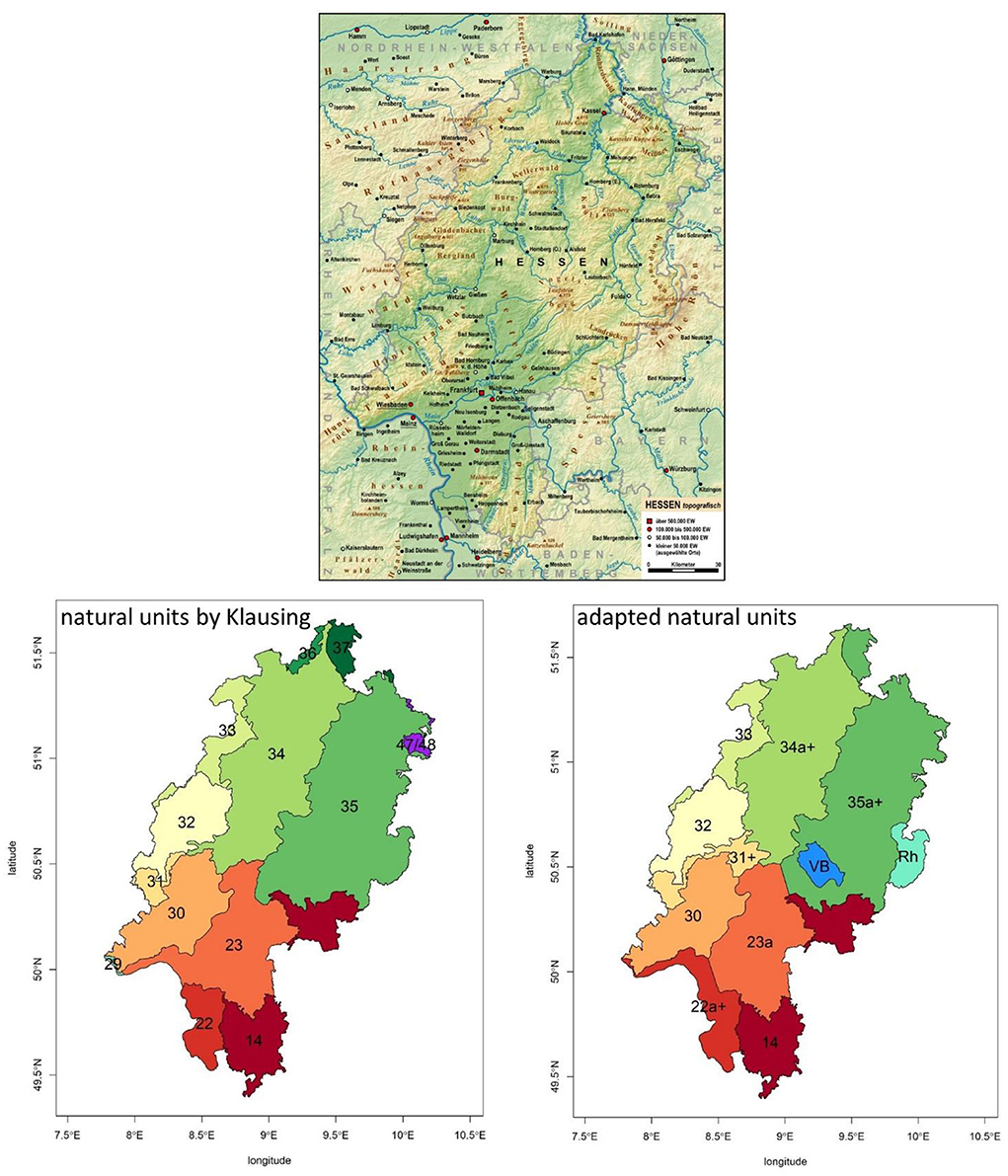
Figure 1. Topographic map of Hesse (top, https://de.wikipedia.org/wiki/Hessen#/media/Datei:Hessen_topografisch_Relief_Karte.png) and map of “natural units” in the second refinement layer (Haupteinheiten) from the original Klausing-classification (bottom left) and resulting adapted natural units for spatial aggregation of climate model output (bottom right). Numbers correspond to: 14, Hessen-Franconian Mountains; 22, Upper-Rhine Lowland; 23, Rhine-Main Lowland; 29, Mittelrhein; 30, Taunus mountains; 31, Gießen-Koblenz-Lahn valley; 32, Westerwald mountains; 33, Bergisch-Sauerland mountains; 34, West Hesse mountain and valley Area; 35, East Hesse mountain area; 36, Weser mountain area; 37, Weser-Leine mountain area; 47/48, Thuringia basin (Klausing, 1988). VB, Vogelsberg; Rh, Rhön; “a”, adjustment of units by changing the boundary of the original unit; “+”, merging of original units.

Several sophisticated methods exist for creating spatial climate patterns, like cluster analysis (e.g., Mahmud et al., 2022) or PCA (e.g., Pineda-Martínez et al., 2007). Alternatively, we started from a well-known and established pattern: the “natural units” (or “landscape units”) as defined by Klausing (Klausing, 1988) (Figure 1, bottom left). The main reason was to use a concept that is readily understandable for many users, not only in climate impact research, but also outside science: in policy and society.

According to climate modeling advice, we aimed for creating spatial units that comprised at least nine grid cells (of the 5 km resolution) for any spatial unit. The Klausing natural units are defined for all of Germany, but we used only the Hesse-part of them. The natural units are based on a large-scale climatological mapping (within central Europe). Finer scale differentiation (i.e., in Hesse) draws on geological information. We thus started our exercise with testing the representativeness of the finer scale (second order) natural units for climatological values. The natural units have the advantage of well-defined physical, geographic, and geologic areas. These areas correspond well with characteristic and well-known regions in Hesse (e.g., low-lying “Wetterau” for apple orchards, Rhine plain “Hessisches Ried” for vegetables growing or the viticultural area “Rheingau” along the “Mittelrhein” in the Rhineland slate mountains), but they do not match administrative units. They neither match hydrological units, which typically span areas from source regions in mountainous terrain to the river mouth in a lowland region, even though in some areas borders of hydrological units match borders of the natural units.

Natural units from HYRAS data

To identify climatological units based on Klausing's natural units, we used HYRAS data, a high-resolution (5 × 5 km) gridded dataset of daily mean (T_mean), minimum (T_min) and maximum (T_max) temperature, precipitation (PR), and relative humidity (RelHum) (Rauthe et al., 2013; Frick et al., 2014; Razafimaharo et al., 2020). Based on these daily data, we calculated long-term seasonal means (sums for precipitation, respectively) for the time period 1951–2010. Additionally, we determined the following meteorological parameters per calendar year: ice days (T_max < 0°C), frost days (T_min < 0°C), summer days (T_max > 25°C), hot days (T_max > 30°C), very hot days (T_max > 35°C), and tropical nights (T_min > 20°C).

When selecting the parameters to be considered in the study with HYRAS data, it was ensured that the parameters are available in the high-resolution data of the regional climate models to which the methodology will eventually be applied. In this way, a consistent data set aggregated to natural units can be provided for Hesse.

First, the natural area means based on Klausing's natural units (second order) were calculated for the listed parameters by weighting the individual cell values according to their area percentage in the respective natural area of Hesse:

$\begin{array}{l}{X}^n=\frac{{\displaystyle \sum w_{ij}^n{X}_{ij}}}{{\displaystyle \sum w_{ij}^n}}\end{array}$

with

$w_{ij}^n:$ Area percentage of the grid cell (i,j) in the natural unit n,

X_ij: Calculated parameter in grid cell (i,j).

In the next step, the deviation from the natural area mean Xⁿ for each parameter was investigated in each grid cell. For reducing the residual deviations, the natural units were adapted.

The decision-structure for adapting the natural units used seasonal and half-yearly mean temperature fields in the first step and aimed for reducing the residual deviations. The decision of redistributing grid-cells from one natural unit to another was made under the following premises (in this order):

1. Keep the alterations as small as possible, to preserve the structure of the original units as well as possible;

2. for units with only a few grid-boxes in Hesse, check if they can be matched with neighboring units to fulfill the area size criterion (at least nine grid boxes of the 5 km resolution fields);

3. check, if distributing the grid cell to a neighboring unit reduces the residual error field;

4. check, if a higher order natural unit (third order) exists, that matches the error pattern and is still large enough to fulfill the area size criterion;

5. if necessary, combine third order units or add an appropriate single grid cells to fulfill the size criterion.

We processed these steps using the seasonal and half-yearly mean temperature field and thereafter checked if the resulting units reduced the residual errors in the other parameter fields, too. This was the case, so we kept the units as determined from mean temperature. Examples of the resulting error fields for mean temperature and summer precipitation are given in Figure 3.

As an example, Figure 2 shows the spatial distribution of the long-term mean air temperature over the winter period from October to March for Hesse. The original classification of the Hessian natural units according to Klausing already corresponds well with the spatial structure of the temperature field. This is due to the fact, that Klausing's natural classification is not based on administrative units, but on scientific data, which in particular takes into account the geography and thus also the climatological differences in Hesse. For example, the lower temperatures in the Hessen-Franconian Mountains are well-distinguished from the northern Upper-Rhine Lowland and the Rhine-Main lowlands. The slightly higher temperatures in the Giessen-Koblenz Lahn Valley are also mapped in a separate natural unit, separated from the Taunus in the south and the Westerwald in the north.

FIGURE 2

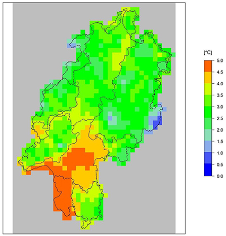
Figure 2. Monthly means of the air temperature in Hesse averaged over the period from 1951 to 2010 and over the winter period from October to March based on HYRAS data. The natural units of Hesse according to Otto Klausing are shown as polygons in black.

On the other hand, it can also be seen that smaller-scale structures are missing from the original classification by Klausing. For example, the Rhön and the Vogelsberg stand out with lower temperatures and thus also fewer summer days and higher precipitation than in the assigned rest of the East Hesse mountain area.

By looking at the grid point-specific deviation from the respective assigned natural area mean, the local differences become clearer and by adjusting the natural unit classification, improvements in the subdivision can be made visible in the form of smaller deviations. This approach is illustrated in Figure 3. Whereas, with an underlying subdivision according to Klausing, deviations of −2 to −2.5 K were recorded for the Vogelsberg and the Rhön (Figure 3, top right), after separating these two regions the deviations in temperature could be reduced to −1 K (Figure 3, bottom right).

FIGURE 3

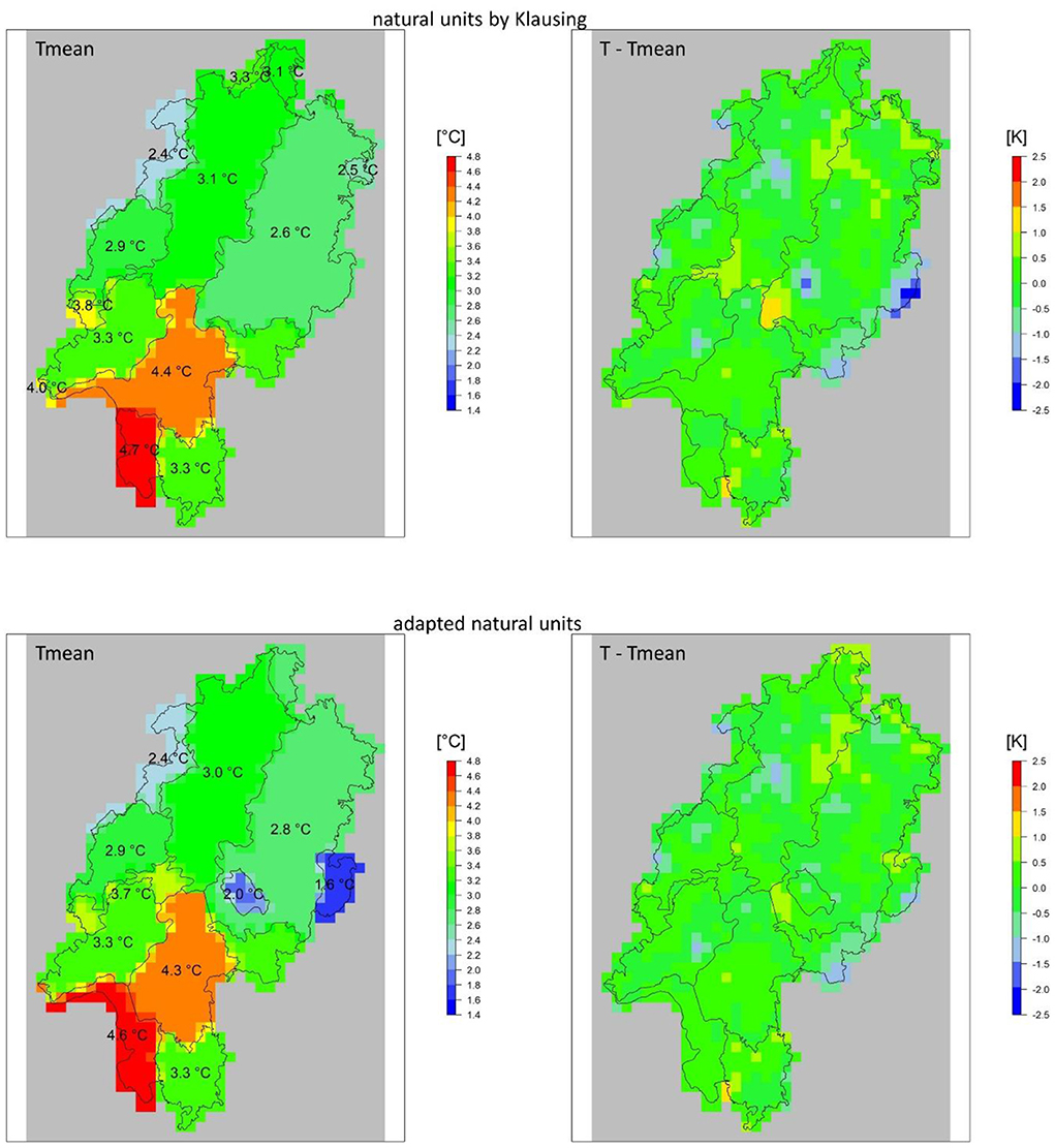
Figure 3. (Left) Multi-year (1951–2010), over the winter period (October–March) and over the natural units averaged monthly means of the air temperature in Hesse based on HYRAS data (T_mean). (Right) Grid point-specific deviations from the long-term natural units mean of the air temperature in Hesse averaged over the winter period (T – T_mean). The natural units of Hesse used for the averaging are drawn in black as polygons (top: natural units according to Otton Klausing, bottom: adapted natural units).

That these separations lead to an improvement is also confirmed in the other selected parameters such as precipitation (Figure 4). When using Klausing's original subdivision, the higher summer precipitation in the Vogelsberg and the Rhön compared to the rest of the East Hesse mountain area of 15–25 mm can be clearly seen. After separating these two areas, the deviations here can be reduced to <10 mm.

FIGURE 4

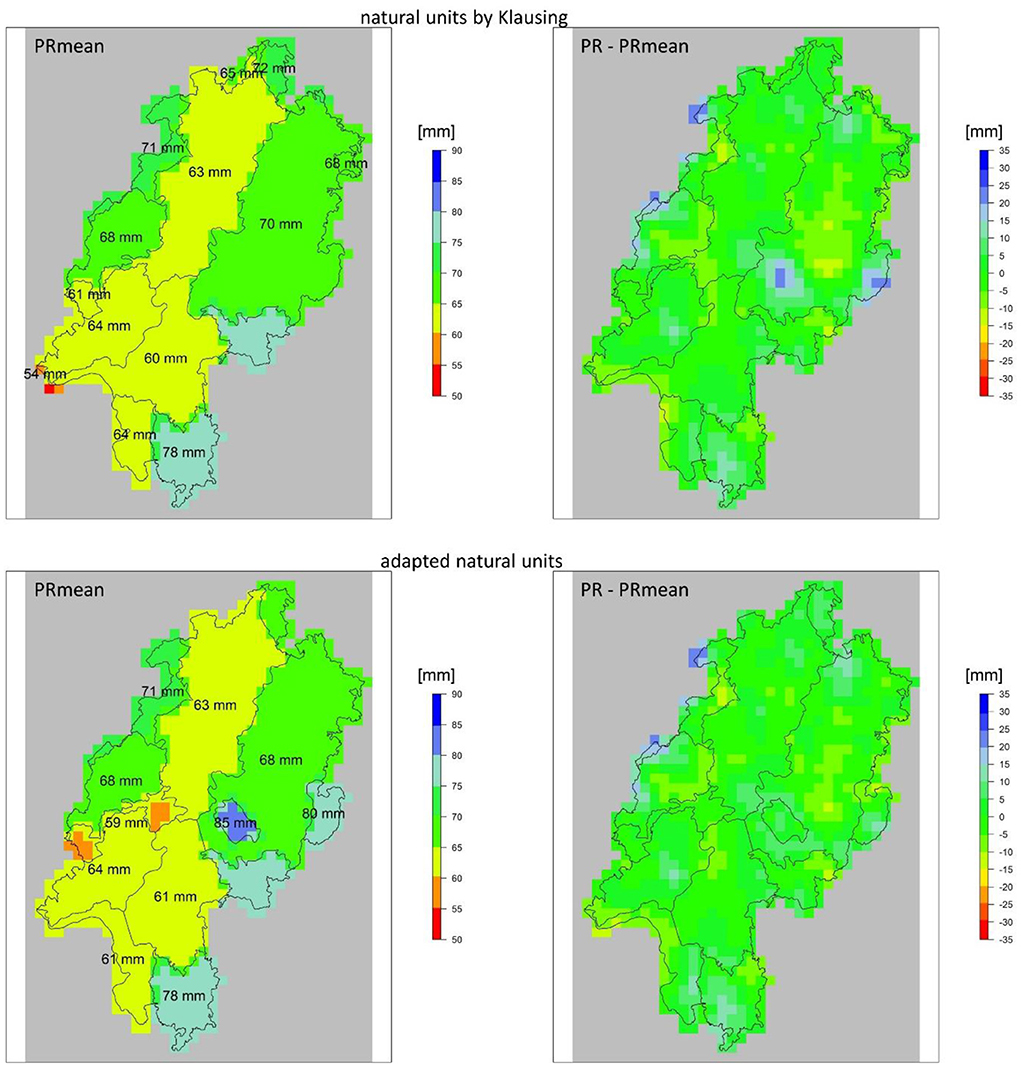
Figure 4. (Left) Multi-year (1951–2010), over the summer period (April–September) and over the natural units averaged monthly sums of precipitation in Hesse based on HYRAS data (PR_mean). (Right) Grid point-specific deviations from the long-term natural units mean of precipitation in Hesse averaged over the summer period (PR – PR_mean). The natural units of Hesse used for the averaging are drawn in black as polygons [(top) natural units according to Otton Klausing, (bottom) adapted natural units].

This procedure was carried out taking into account all the selected meteorological variables, so that finally an adapted classification of the natural units was obtained with the following maximum deviations in the individual meteorological variables: T (−1.7 K/+1.6 K), T_min (−1.1 K/+1.4 K), T_max (−2.5 K/+1.7 K), PR (−18 mm/+34 mm), and RelHum (−3%/+4%).

In the end, the following alterations were made to the Klausing units for further use of the climate spatial units:

1. The Rhön and the Vogelsberg as low mountain ranges, which belong to the East Hesse mountain area (No. 35), should be considered as separate natural units. Here, due to the blocking effect of the mountains and their altitude, precipitation is significantly higher and temperatures lower than in the rest of the East Hesse mountain area.

2. In the transition from the Rhine-Main Lowland (No. 23) to the East Hesse mountain area (No. 35), the southwestern part of the western lower Vogelsberg should be assigned to the Rhine-Main Lowland, since here the long-term seasonal monthly mean temperature is higher than the area mean of the East Hesse mountain area.

3. The Rhine valley, which according to Klausing is assigned to the Upper-Rhine Lowland (No. 22) and the Rhine-Main Lowland (No. 23), was completely integrated into the Upper-Rhine Lowland (No. 22) and merged with the very small natural unit of the Mittelrhein (No. 29), which is covered by only three grid cells.

4. The Weser mountain area (No. 36) was integrated into the West Hesse mountain and valley Area (No. 34).

5. The Thuringia basin (No. 47/48) and the Weser-Leine mountain area (No. 37) was merged with the East Hesse mountain area (No. 35).

6. The Giessen Lahn valley, which according to Klausing is assigned to the West Hesse mountain and valley Area (No. 34), was instead merged with the Giessen-Koblenz Lahn valley (No. 31), because the long-term seasonal monthly mean temperature is higher and the long-term seasonal monthly mean relative humidity is lower than the area mean of the West Hesse mountain and valley Area (No 34).

Figure 1 (bottom right) shows the map of the newly adapted natural units.

Subsequently, these adjusted natural units were used for post-processing of climate model outputs in natural units.

Regional climate model data in natural units

We used regional climate model data from the projects ReKliEs-De (Huebener et al., 2017a) and EURO-CORDEX (Jacob et al., 2013) in a 0.11° resolution (approximately 12 km). The data was then bias corrected (Cannon, 2018) and disaggregated to a 5 km resolution by the German Weather Service (DWD) (Krähenmann et al., 2021). The disaggregation process included high-resolution spatial and climatological information and is therefore of sufficiently high spatial quality to be used on this scale.

We provided the following data spatially aggregated at a level of natural units as described above:

• for the reference period 1971–2000 (control run) and for the period 2071–2100 (RCP2.6 and RCP8.5):

° single values for each month from January 2071 to December 2100

° climatological monthly values (averaged for 2071–2100)

• difference between single month values for the period 2071–2100 and climatological monthly values simulated by the respective model for the reference period (1971–2000).

for the parameters

• daily mean temperature (T_mean) as monthly mean

• minimum temperature (T_min) as monthly mean

• maximum temperature (T_max) as monthly mean

• precipitation (PR) as monthly sum

• relative humidity (RelHum) as monthly mean

• number of days per calendar year:

° ice days (T_max < 0°C)

° frost days (T_min < 0°C)

° summer days (T_max > 25 °C)

° hot days (T_max > 30 °C)

° very hot days (T_max > 35 °C)

° tropical nights (T_min > 20 °C)

The cartographical projection of the data is Lambert conformal conic (LCC) and the data format is NetCDF, readable and processable in standard GIS programs.

Lessons learned

The aggregation method presented here aims at improving the spatial representativeness of gridded model output while maintaining the averaging process for insuring robustness of the results (i.e., eliminating spurious single grid cell values or systematic shifts within a natural unit). We applied only relatively minor, albeit essential alterations to minimize the relative errors of the mean values compared to the single cell values. The procedure thus seems a viable path for other regions, too, for improving spatial representativeness of climate model data.

Additionally, the provision of monthly values for the future period (single month values for each year from 2071 to 2100, each as deviation from the simulated climatological monthly value of the reference period 1971–2000) now allows to analyze consecutive or combined events in the future on monthly time scales, even without the knowledge and capacity to handle the direct climate model output.

Such events might include consecutive dry summers or combinations of hot and dry spring months. Possible applications could be in fields like hydrology (e.g., filling of reservoirs, groundwater recharge), agriculture (e.g., irrigation needs), forestry (e.g., conditions for bark beetle infestation or fire weather), health (e.g., habitat for invasive mosquitos), or ecosystem services (e.g., evaporative cooling from urban green spaces during dry summers).

A large number of impact research methods require daily data, particularly when considering extreme heat or heavy precipitation events. These events cannot be resolved by the monthly data. We don't expect the method to work equally well for daily data. On the daily time-scale spatial variability is much larger (particularly for rainfall) and events like temperature inversions defy their expression in the simple spatial methods used here. Thus, a number of impact relevant extremes occurring on the daily time-scale cannot be assessed with these data.

Assessing the study results, on the “pro” side, we were positive surprised how well the original natural units fit with a number of relevant quantities for climate and climate impact analyses. The good fit of mean temperature with the adjusted natural units was expected, since the topography—particularly height above sea level—strongly controls mean temperatures. However, minimum and maximum temperatures, precipitation, and relative humidity are not as clearly controlled by this parameter. This is an added value of the results presented here.

The provision of data aggregated to the adjusted natural units presented here results in a much higher plausibility of local climate data compared to aggregation over rectangular areas. With this product, downstream users can now select a natural unit as surrogate for a local grid-box and use the data for their further analyses.

On the “con” side, spatial variations within the natural units are not resolved and the monthly resolution will still be insufficient for some impact assessments. This limits the use of the data for certain impact research questions. For some impact research questions, however, it might be possible to use monthly data even though current impact models use daily data as input. In these cases, the impact researchers might further develop their methods or models to cope with monthly data, and might in some cases even improve the robustness of the results. Here, we need further developments to bridge the remaining gap between the requirements of the impact research community and the climate modeling community.

Summary and conclusion

There is still a considerable gap between climate data, particularly climate model results, and the user needs for climate information to derive climate adaptation measures. The gap has many dimensions: from the nature of climate simulations as only one possible realization of the climate system, different future scenarios, model deficiencies, biases, spatial and temporal resolution, to unwieldy data-formats.

There are numerous ongoing efforts to improve the usability and user-orientation of climate information and climate services (e.g., Alexander and Bruno Soares, 2017; Buontempo et al., 2018; Le et al., 2020; Williams and Jacob, 2021), particularly within the Global Framework on Climate Services (Hewitt et al., 2012). We particularly welcome and support the efforts of transdisciplinary research, of co-production of climate knowledge and of integration of local knowledge to understanding climate change and its impacts (e.g., Buontempo et al., 2018; Hewitt et al., 2021; Neset et al., 2021; Williams and Jacob, 2021). The example presented here may be considered as a small contribution within the field of spatial integration of climate data and information for use in climate impact research (as discussed in the review paper, Giuliani et al., 2017). Our effort is part of the information transfer chain, insofar as it purposefully uses a well-known, if simple, concept (the natural units or landscape units) instead of more sophisticated methods like cluster analysis or PCA. Thus, we take a step toward making the data easier to integrate with data from other disciplines or from outside science. It may also be considered part of the information chain, that the work presented here was incentivized and commissioned by a local environmental agency, so in fact as a transdisciplinary effort.

In this paper, we focus on the resolution of climate model output in space and time. We propose a compromise between the positions of the climate modeling community and of the user community (or communities). The impetus to this effort resulted from discussions with climate impact modelers, presenting their challenges in using climate model data.

The German federal state Rhineland-Palatinate also uses natural units as analysis units for the display of climate and climate change facts (see RLPKK, 2022). Here, the original natural units—as derived from the geological properties—are used to calculate area mean values without prior changes to the areas. This leads to a few natural units, which combine different climatological regimes, like the unit “Taunus mit Lahntal” (which covers areas in both federal states, Hesse and Rhineland-Palatinate), which contains part of a mountain range (Taunus) as well as a river valley (Lahn-Valley); for Hesse we used a sub-division between the two parts of this unit. Additionally, for Rhineland-Palatinate only climatological 30-year averages are on display.

Solutions to improve the usability of climate model data differ according to the intended use. There is no one method to satisfy all user demands. The compromise solutions for improving spatial and temporal resolution presented in this paper only bridge part of the gap between climate simulation data and impact research needs. While this might suffice for some analyses, clearly further steps are needed to bridge this gap to the satisfaction of climate modelers as well as impact researchers. However, this bridging process needs to come from both sides: from the climate modeling community in improving their products as well as from the impact modeling community (Kreienkamp and Huebener, 2021; Sutmöller et al., 2021). Some climate model limitations cannot be overcome by improving the models or post-processing the output data. They stem e.g., from scenario uncertainty or internal climate variability. Thus, a dialog between climate data providers and users should always be part of climate data provision (Van den Hurk et al., 2018). It will need further model and method development within the impact research community to facilitate optimal use of climate model output and data.

We are confident, that the use of (possibly adjusted) natural units increases the spatial representativeness of grid-box data and thus the applicability for impact research. We are also confident, that the provision of monthly projection data (as anomaly to monthly climatological means of the reference period) are scientifically sound enough to allow impact analyses of consecutive or combined events. We encourage other climate data providers to test these methods and to evaluate their applicability to further data sets.

Data availability statement

The raw data supporting the conclusions of this article will be made available by the authors, without undue reservation.

Author contributions

HH contributed the general project idea and the concept of this work, JL and UG provided the actual calculation and data provision. All authors contributed to discussing the results and writing the paper.

Funding

This work was funded by the Hessian Agency for Nature Conservation, Environment and Geology under grant number 4501177980.

Acknowledgments

We thank the German Weather Service for data post-processing (bias correction and downscaling to 5 km resolution) and for data provision. We also thank the reviewers and the editor for their comments, which helped improving the paper.

Conflict of interest

Authors JL and UG are employed by MeteoSolutions GmbH. Author HH works at the funding agency HLNUG.

Publisher's note

All claims expressed in this article are solely those of the authors and do not necessarily represent those of their affiliated organizations, or those of the publisher, the editors and the reviewers. Any product that may be evaluated in this article, or claim that may be made by its manufacturer, is not guaranteed or endorsed by the publisher.

References

Alexander, M., and Bruno Soares, M. (2017). Multi-sector requirements of climate information and impact indicators across Europe: Findings from the SECTEUR European-wide survey. Copernicus Climate Change Service. doi: 10.13140/RG.2.2.18132.81282

CrossRef Full Text | Google Scholar

Allen, M. R., Stott, P., Mitchell, J., Schnur, R., and Delworth, T. (2000). Quantifying the uncertainty in forecasts of anthropogenic climate change. Nature 407, 617–620. doi: 10.1038/35036559

PubMed Abstract | CrossRef Full Text | Google Scholar

Bollmeyer, C., Keller, J. D., Ohlwein, C., Wahl, S., Crewell, S., Friederichs, P., et al. (2015). Towards a high-resolution regional reanalysis for the European CORDEX domain. Quart. J. Roy. Meteor. Soc. 141, 1–15. doi: 10.1002/qj.2486

CrossRef Full Text | Google Scholar

Bülow, K., Hübener, H., Keuler, K., Menz, C., Pfeifer, S., Ramthun, H., et al. (2019). User tailored results of a regional climate model ensemble to plan adaption to the changing climate in Germany. Adv. Sci. Res. 16, 241–249. doi: 10.5194/asr-16-241-2019

CrossRef Full Text | Google Scholar

Buontempo, C., Hanlon, H. M., Bruno Soares, M., Christel, I., Soubeyroux, J. M., Viel, C., et al. (2018). What have we learnt from EUPORIAS climate service prototypes? Clim. Serv. 9, 21–32. doi: 10.1016/j.cliser.2017.06.003

CrossRef Full Text | Google Scholar

Cannon, A. J. (2018). Multivariate quantile mapping bias correction: an N-dimensional probability density function transform for climate model simulations of multiple variables. Clim. Dyn. 50, 31–49. doi: 10.1007/s00382-017-3580-6

CrossRef Full Text | Google Scholar

Casanueva Herrera, S., Iturbide, M., Lange, S., Jury, M., Dosio, A., Maraun, D., et al. (2020). Testing bias adjustment methods for regional climate change applications under observational uncertainty and resolution mismatch. Atmos. Sci. Lett. 21:e978. doi: 10.1002./asl.978

CrossRef Full Text | Google Scholar

Chimani, B., Matulla, C., Hiebl, J., Schellander-Gorgas, T., Maraun, D., Mendlik, T., et al. (2020). Compilation of a guideline providing comprehensive information on freely available climate change data and facilitating their efficient retrieval. Clim. Serv. 19, 100179. doi: 10.1016/j.cliser.2020.100179

CrossRef Full Text | Google Scholar

Christel, I., Hemment, D., Bojovic, D., Cucchietti, F., Calvo, L., Stefaner, M., et al. (2017). Introducing design in the development of effective climate services. Clim. Serv. 9, 111–121. doi: 10.1016/j.cliser.06, 002

PubMed Abstract | CrossRef Full Text | Google Scholar

Dalelane, C., Früh, B., Steger, C., and Walter, A. (2018). A Pragmatic approach to build a reduced regional climate projection ensemble for Germany using the EURO-CORDEX 8.5 ensemble. J. Appl. Meteorol. Climatol. 57, 477–491. doi: 10.1175/JAMC-D-17-0141.1

CrossRef Full Text | Google Scholar

Dee, D., Uppala, S., Simmons, A., Berrisford, P., Poli, P., Kobayashi, S., et al. (2011). The era-interim reanalysis: configuration and performance of the data assimilation system. Quart. J. Roy. Meteor. Soc. 137, 553–597. doi: 10.1002/qj.828

CrossRef Full Text | Google Scholar

Deser, C., Lehner, F., Rodgers, K. B., Ault, T., Delworth, T. L., DiNezio, P. N., et al. (2020). Insights from Earth system model initial-condition large ensembles and future prospects. Nat. Clim. Change 10, 277–286. doi: 10.1038/s41558-020-0731-2

CrossRef Full Text | Google Scholar

Deser, C., Terray, L., and Phillips, A. S. (2016). Forced and internal components of winter air temperature trends over North America during the past 50 years: mechanisms and implications. J. Clim. 29, 2237–2258. doi: 10.1175/JCLI-D-15-0304.1

CrossRef Full Text | Google Scholar

Eyring, V., Bony, S., Meehl, G. A., Senior, C. A., Stevens, B., Stouffer, R. J., et al. (2016). Overview of the Coupled Model Intercomparison Project Phase 6 (CMIP6) experimental design and organization. Geosci. Model Dev. 9, 1937–1958. doi: 10.5194/gmd-9-1937-2016

CrossRef Full Text | Google Scholar

Frick, C., Steiner, H., Mazurkiewicz, A., Riediger, U., Rauthe, M., Reich, T., et al. (2014). Central European high-resolution gridded daily data sets (HYRAS): mean temperature and relative humidity. Meteorol. Z. 23, 15–32. doi: 10.1127/0941-2948/2014/0560

CrossRef Full Text | Google Scholar

Giuliani, G., Nativi, S., Obregon, A., Beniston, M., and Lehmann, A. (2017). Spatially enabling the global framework for climate services: reviewing geospatial solutions to efficiently share and integrate climate data and information. Clim. Serv. 8, 44–58. doi: 10.1016/j.cliser.08, 003

CrossRef Full Text | Google Scholar

Goddard, L. (2016). From science to service. Science 353, 1366–1367. doi: 10.1126/science.aag3087

PubMed Abstract | CrossRef Full Text | Google Scholar

Hawkins, E., Smith, R. S., Gregory, J. M., and Stainforth, D. A. (2016). Irreducible uncertainty in near-term climate projections. Clim. Dyn. 46, 3807–3819. doi: 10.1007/s00382-015-2806-8

CrossRef Full Text | Google Scholar

Hewitt, C., Bessembinder, J., Buonocore, M., Dunbar, T., Garrett, N., Kotova, L., et al. (2021). Coordination of Europe's climate-related knowledge base: networking and collaborating through interactive events, social media and focussed groups. Clim. Serv. 24:100264. doi: 10.1016/j.cliser.2021.100264

CrossRef Full Text | Google Scholar

Hewitt, C., Mason, S., and Walland, D. (2012). The global framework for climate services. Nat. Clim. Change 2, 831–832. doi: 10.1038/nclimate1745

CrossRef Full Text | Google Scholar

Huebener, H., Bülow, K., Fooken, C., Früh, B., Hoffmann, P., Höpp, S., et al. (2017a). ReKliEs-De Ergebnisbericht (in German). Universitat Hohenheim.

Google Scholar

Huebener, H., Keuler, K., Pfeifer, S., Ramthun, H., Spekat, A., Steger, C., et al. (2017b). Deriving user-informed climate information from climate model ensemble results. Adv. Sci. Res. 14, 261–269. doi: 10.5194/asr-14-261-2017

CrossRef Full Text | Google Scholar

Jacob, D., Petersen, J., Eggert, B., Alias, A., Bøssing Christensen, O., Bouwer, L., et al. (2013). EURO-CORDEX: new high-resolution climate change projections for European impact research. Reg. Environ. Change 14, 563–578. doi: 10.1007/s10113-013-0499-2

CrossRef Full Text | Google Scholar

Johns, T. C., Royer, J.-F., Höschel, I., Huebener, H., Roeckner, E., May, M. W., et al. (2011). Climate change under aggressive mitigation: the ENSEMBLES multi-model experiment. Clim. Dyn. 37, 1975–2003. doi: 10.1007/s00382-011-1005-5

CrossRef Full Text | Google Scholar

Kay, J. E., Deser, C., Phillips, A., Mai, A., Hannay, C., Strand, G., et al. (2015). The Community Earth System Model (CESM) large ensemble project: a community resource 44 for studying climate change in the presence of internal climate variability. Bull. Amer. Meteorol. Soc. 96, 1333–1349. doi: 10.1175/BAMS-D-13-00255.1

CrossRef Full Text | Google Scholar

Klausing, O. (1988). Die Naturräume Hessens. Umweltatlas Hessen des Hessischen Landesamtes für Umwelt und Geologie. Karte zu den Naturräumen Hessens. Available online at: https://web.archive.org/web/20141010022448/http://atlas.umwelt.hessen.de/atlas/naturschutz/naturraum/karten/m_3_2_1.htm (accessed January 26, 2022); Legende zu den Naturräumen Hessens: https://web.archive.org/web/20201009172346/http://atlas.umwelt.hessen.de/atlas/naturschutz/naturraum/texte/ngl-sy.htm (Accessed January 26 2022).

Google Scholar

Kotlarski, S. (2014). Regional climate modelling on European scales: a joint standard evaluation of the EURO-CORDEX RCM ensemble. Geosci. Model Dev. Discuss. 7, 217–293. doi: 10.5194/gmdd-7-217-2014

CrossRef Full Text | Google Scholar

Krähenmann, S., Walter, A., and Klippel, L. (2021). Statistische aufbereitung von klimaprojektionen: downscaling und multivariate bias-adjustierung (in German). Berichte des Deutschen Wetterdienstes 2021:254.

Google Scholar

Kreienkamp, F., and Huebener, H. (2021). Aspekte der Nutzung von regionale Klimaprojektionsdatensätzen (in German with English abstract). Promet 104, 5–8. doi: 10.5676/DWD_pub/promet_104_01

CrossRef Full Text | Google Scholar

Kreienkamp, F., Huebener, H., Linke, C., and Spekat, A. (2013). Good practice for the usage of climate model simulation results – a discussion paper. Environ. Syst. Res. 1:9. doi: 10.1186/2193-2697-1-9

CrossRef Full Text | Google Scholar

Le, T., Perrels, A., and Cortekar, J. (2020). European climate services markets – conditions, challenges, prospects, and examples. Clim. Serv. 17:100149. doi: 10.1016./j.cliser.2020.100149

CrossRef Full Text | Google Scholar

Lemos, M. C., Kirchhoff, C. J., and Ramprasad, V. (2012). Narrowing the climate information usability gap. Nat. Clim. Change 2, 789–794. doi: 10.1038/nclimate1614

CrossRef Full Text | Google Scholar

Mahmud, S., Sumana, F. M., Mohsin, M., and Khan, M. H. R. (2022). Redefining homogenous climate regions in Bangladesh using multivariate clustering approaches. Nat. Hazards 111, 1863–1884. doi: 10.1007/s11069-021-05120-x

CrossRef Full Text | Google Scholar

Marotzke, J., and Forster, P. M. (2015). Forcing, feedback and internal variability in global temperature trends. Nature 517, 565–570. doi: 10.1038/nature14117

PubMed Abstract | CrossRef Full Text | Google Scholar

Neset, T.S, Wilk, J., Cruz, S., Graça, M., Rød, J. K., et al. (2021). Co-designing a citizen science climate service. Clim. Serv. 24, 100273. doi: 10.1016./j.cliser.2021.100273

CrossRef Full Text | Google Scholar

Pérez-Zanón, N., Caron, L. P., Terzago, S., Van Schaeybroeck, B., Lledó, L., Manubens, N., et al. (2021). The CSTools (v4.0) Toolbox: from climate forecasts to climate forecast information. Geosci. Model Dev. doi: 10.5194/gmd-2021-368

CrossRef Full Text | Google Scholar

Pineda-Martínez, L. F., Carbajal, N., and Medina-Roldán, E. (2007). Regionalization and classification of bioclimatic zones in the central-northeastern region of México using principal component analysis (PCA). Atmósfera 20.

Google Scholar

Raoult, B., Bergeron, C., López Alós, A., Thépaut, J.-.N, and Dee, D. (2017). Climate service develops user-friendly data store. ECMWF Newslett. 151, 1–9. doi: 10.21957/p3c285

CrossRef Full Text | Google Scholar

Rauthe, M., Steiner, H., Riediger, U., Mazurkiewicz, A., and Gratzki, A. A. (2013). Central European precipitation climatology – Part I: generation and validation of a high-resolution gridded daily data set (HYRAS). Meteorol. Z. 22, 235–256. doi: 10.1127/0941-2948/2013/0436

CrossRef Full Text | Google Scholar

Razafimaharo, C., Krähenmann, S., Höpp, S., Rauthe, M., and Deutschländer, T. (2020). New heigh-resolution gridded dataset of daily mean, minimum and maximum temperature and relative humidity for Central Europe (HYRAS). Ther. Appl. Climatol. 142, 1531–1553. doi: 10.1007/s00704-020-03388-w

CrossRef Full Text | Google Scholar

RLPKK. (2022). Rheinland-Pfalz Kompetenzzentrum für Klimawandelfolgen. Available online at: https://www.kwis-rlp.de/daten-und-fakten/klimawandel-zukunft/ (accessed January 26, 2022).

Google Scholar

Rössler, O., Fischer, A. M., Huebener, H., Benestad, R., Christodoulides, P., Maraun, D., et al. (2017). Challenges to link climate change data provision and user needs - perspective from the COST-VALUE initiative. Int. J. Climatol. 39, 3704–3716. doi: 10.1002/joc.5060

CrossRef Full Text | Google Scholar

Suhari, M., Dressel, M., and Schuck-Zöller, S. (2022). Challenges and best practices of co-creation: a qualitative interview study in the field of climate services. Clim. Serv. 25:100282. doi: 10.1016/j.cliser.2021.100282

CrossRef Full Text | Google Scholar

Sutmöller, J., Schönfelder, E., and Meesenburg, H. (2021). Perspektiven der Anwendung von Klimaprojektionen in der Forstwirtschaft (in German with English abstract). Promet 104, 47–53. doi: 10.5676/DWD_pub/promet_104_07

CrossRef Full Text | Google Scholar

Tart, S., Groth, M., and Seipold, P. (2020). Market demand for climate services: an assessment of users' needs. Clim. Serv. 17, 100109. doi: 10.1016/j.cliser.2019.100109

CrossRef Full Text | Google Scholar

Uppala, S. (2001). ECMWF ReAnalysis 1957-2001 ERA-40. European Centre for Medium-Range Weather Forecasts (ECMWF). Available online at: https://www.ecmwf.int/sites/default/files/elibrary/2001/12879-ecmwf-reanalysis-1957-2001-era-40.pdf

Google Scholar

Van den Hurk, B., Hewitt, C., Jacob, D., Bessembinder, J., Doblas-Reyes, F., Döscher, R., et al. (2018). The match between climate service demands and earth system models supplies. Clim. Serv. 12, 59–63. doi: 10.1016/j.cliser.2018.11.002

CrossRef Full Text | Google Scholar

Vautard, R., Kadygrov, N., Iles, C., Bülow, K., Jacob, D., Teichmann, C., et al. (2020). Evaluation of the large EURO-CORDEX regional climate model ensemble. J. Geophys. Res. Atmos. 126:e2019JD032344. doi: 10.1029./2019JD032344

CrossRef Full Text | Google Scholar

Williams, D. S., and Jacob, D. (2021). From participatory to inclusive climate services for enhancing societal uptake. Clim. Serv. 24:100266. doi: 10.1016./j.cliser.2021.100266

CrossRef Full Text | Google Scholar

Zier, C. H., Bäse, F., and Komischke, H. (2021). Ein Verfahren zur Plausibilisierung und Bewertung regionaler Klimaprojektionen (An assessment of regional climate projections, in German with English abstract). Promet 104, 9–18. doi: 10.5676/DWD_pub/promet_104_02

CrossRef Full Text | Google Scholar