 Colette Kerry
 Moninya Roughan
 Joao Marcos Azevedo Correia de Souza2
95% of researchers rate our articles as excellent or good
Learn more about the work of our research integrity team to safeguard the quality of each article we publish.
Find out more
ORIGINAL RESEARCH article
Front. Clim. , 28 October 2022
Sec. Climate, Ecology and People
Volume 4 - 2022 | https://doi.org/10.3389/fclim.2022.980990
This article is part of the Research Topic Advances in Marine Heatwave Interactions View all 18 articles
Marine heatwaves can have devastating ecological and economic impacts and understanding what drives their onset is crucial to achieving improved prediction. A key knowledge gap exists around the subsurface structure and temporal evolution of MHW events in continental shelf regions, where impacts are most significant. Here, we use a realistic, high-resolution ocean model to identify marine heatwaves using upper ocean heat content (UOHC) as a diagnostic metric. We show that, embedded in the inter-annual variability of UOHC across the Tasman Sea, regional UOHC around New Zealand varies at short temporal and spatial scales associated with local circulation which drives the onset of extreme events with median duration of 5–20 days. Then, using a novel application of Adjoint Sensitivity Analysis, we diagnose the regional drivers of extreme UOHC events and their 3-dimensional structure. We compute the sensitivity of UOHC to changes in the ocean state and atmospheric forcing over the onset of MHW events using ensembles of between 34 and 64 MHW events across 4 contrasting regions over a 25-year period. The results reveal that changes in regional UOHC on short (5-day) timescales are largely driven by local ocean circulation rather than surface heat fluxes. Where the circulation is dominated by boundary currents, advection of temperature in the mixed layer dominates the onset of extreme UOHC events. Higher magnitude MHW events are typically associated with shallower mixed layer and thermocline depths, with higher sensitivity to temperature changes in the upper 50–80 m. On the west coast, where boundary currents are weak, UOHC extremes are sensitive to density changes in the upper 1,000 m and likely caused by downwelling winds. Our results highlight the importance of understanding the different temporal and spatial scales of UOHC variability. Understanding the local circulation associated with heat content extremes is an important step toward accurate MHW predictability in economically significant shelf seas.
Marine heatwaves (MHWs) refer to extended periods of anomalously warm ocean temperatures and can have devastating impacts on marine biodiversity and ecosystems and major economic impacts on regional fisheries. MHWs have already become more frequent, more intense and longer-lasting in the past few decades, and this trend is expected to accelerate under further global warming (Frölicher et al., 2018; Oliver et al., 2018a,b; Darmaraki et al., 2019b). It is clear that MHWs can be driven by a number of processes occurring over various temporal and spatial scales which determine their predictability (e.g., Jacox et al., 2019). Understanding the physical processes that give rise to MHWs is key to predicting the likelihood, severity and timing of these events. Ocean heat content varies across temporal and spatial scales, driven by climate variations and local processes (Holbrook et al., 2019). In coastal regions, understanding this variability and the influence of both climate- and local-scale processes in driving ocean heat content extremes is key to predicting MHWs.
Enhanced oceanic heat content on regional- and basin-scales can act as a preconditioner to increased likelihood of MHWs (e.g., Behrens et al., 2019). A global assessment of MHWs found coherent relationships between MHWs and dominant climate modes, except in Western Boundary Current regions where the energetic and non-linear nature of these current regions make ocean-climate relationships complex (Holbrook et al., 2019). In the southwest Pacific, Bowen et al. (2017) find that SST around New Zealand (NZ) is connected to regional processes over a wide area of the South Pacific. They show that the temperature and upper ocean heat content are highly correlated on the west and east coasts of NZ on interannual timescales despite marked differences in current regions. Sutton and Bowen (2019) show that significant interannual variability in upper ocean temperature is coherent over a large area of the Tasman Sea north of the Subtropical Front. MHWs off Western Australia have been associated with large-scale subsurface temperature anomalies extending from the western Pacific into the tropical eastern Indian Ocean (Ryan et al., 2021). SW Pacific SST anomalies due to El Niño events contribute to triggering MHWs off southeast Queensland (Heidemann and Ribbe, 2019), and NE Pacific MHWs have been associated with widespread warm SST anomalies (Scannell et al., 2020). How these large scale temperature anomalies influence shelf and coastal MHWs is complex and likely region- and case-specific.
Embedded in the large-scale variations in ocean heat content, regional and coastal MHWs at smaller spatial scales have been shown to be driven by shifts in warm ocean currents and eddy activity. UOHC anomalies in the East Australian Current (EAC) southern extension have been shown to be associated with the poleward penetration of the EAC, modulated by both a weaker, more stable EAC and incoming westward-propagating Rossby waves (Li et al., 2020, 2022). Indeed, increased poleward transport in the EAC southern extension is found to be the dominant driver of MHWs off eastern Tasmania (Oliver et al., 2017, 2018b). MHWs over the Northwest Atlantic continental shelf and slope were shown to be driven by a combination of atmospheric and oceanic drivers, specifically warm core rings shed by the Gulf Stream (Perez et al., 2021). Analysis of coastal MHW events around southern Africa found that MHWs were predominantly caused by warm Agulhas Current water forced onto the continental shelf and warm atmospheric temperatures combined with onshore winds (Schlegel et al., 2017). They found that fine-scale warm core eddies were commonly associated with MHW events. Kerry et al. (2022) show that oceanic eddies are the dominant drivers of UOHC variability at intra-annual scales around NZ. On the northeast US continental shelf, both large scale atmospheric forcing, and local along- and cross-shelf ocean advection cause extreme warm ocean temperatures (Chen et al., 2015). For coastal MHWs on the southeast Australian continental shelf, Schaeffer and Roughan (2017) show that anomalously warm temperatures at depth are driven by local downwelling favorable winds that mix the water column and reduce the stratification. Clearly an understanding of the local processes at play is key to predicting regional and coastal MHWs.
While MHWs are typically characterized by SST anomalies (due to data availability), clearly an understanding of subsurface temperature and ocean heat content is crucial to understanding MHWs and their ecological impacts. Schaeffer and Roughan (2017) show that SST is insufficient to fully understand MHWs which (in 100 m water depth off southeastern Australia) often extend the full depth of the water column, with a maximum intensity and duration below the surface. Elzahaby and Schaeffer (2019) showed that MHWs in the Tasman Sea can extend to depths of more than 1,200 m, with greater temperature anomalies at depth than their surface signal. They show that these events occur predominantly within warm-core mesoscale eddies, which typically extend below 1,000 m (Rykova et al., 2017; Kerry and Roughan, 2020). Off Western Australia, MHWs driven by the poleward advection of warm water in the Leeuwin Current are distinctively deeper than atmospherically-driven events (Benthuysen et al., 2014; Ryan et al., 2021). In the Mediterranean Sea, subsurface MHWs are typically of higher intensity and severity relative to surface MHWs, probably due to their longer durations (Darmaraki et al., 2019a). Perez et al. (2021) show that meanders of the Gulf Stream onto the Northwest Atlantic continental shelf and slope resulted in large temperature anomalies that extend below 300 m depth and can persist on the shelf for several months. Penetration of subsurface temperature anomalies through the mixed layer depth can occur through a variety of processes and it is possible for these anomalous temperatures to remain from one season to the next, even after the signal of a MHW has dissipated from the surface (Scannell et al., 2020; Jackson et al., 2021). While mixed layer heat budgets are often used to diagnose MHW drivers (e.g., Elzahaby et al., 2021, 2022), it is clear that MHWs often extend below the mixed layer and the influence of salinity and subsurface water mass properties are important (e.g., Ryan et al., 2021) but often overlooked (Holbrook et al., 2020). For these reasons a more thorough understanding of the sub-surface structure of MHWs and UOHC anomalies as well as the temporal evolution of their onset and decay is required.
Here, we use the NZ region as a case study to reveal the dominate drivers of regional MHWs. NZ is located in the southwest Pacific, a known ocean warming hotspot and a region of large-scale coherent ocean heat content and thermocline variability (Bowen et al., 2017). Embedded in the large scale context, NZ experiences complex boundary current circulation (Figure 1a, Stevens et al., 2021) likely to influence how the large scale temperature extremes are experienced in its shelf and coastal waters.
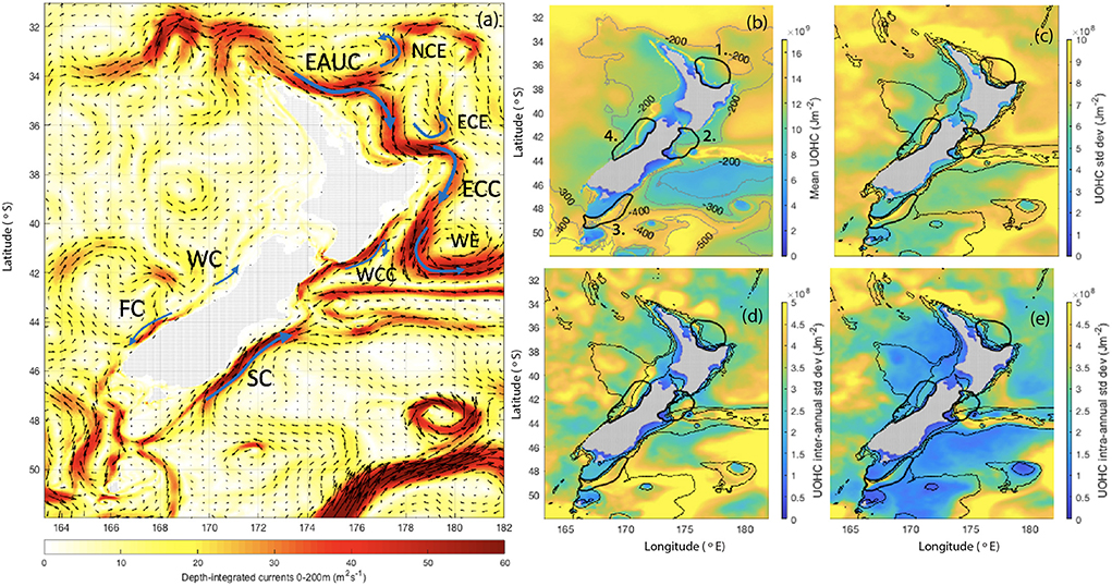
Figure 1. Depth-integrated currents from 0 to 200 m with schematic of New Zealand's major currents (a), mean UOHC with 90th percentile thermocline depth contours (b), standard deviation of UOHC (c), standard deviation of UOHC low-pass filtered at inter-annual periods (d) and standard deviation of UOHC band-pass filtered from 60 to 250 days (e), computed from the MOANA Ocean Hindcast. The four regions chosen for MHW analysis are labeled on (b), 1. Bay of Plenty, 2. Kaikoura, 3. Stewart Plateau and Snares Shelf 4. Hokitika. The 100, 400, and 1,000 m depth contours are shown on (c–e). EAUC, East Auckland Current; NCE, North Cape Eddy; ECC, East Cape Current; ECE, East Cape Eddy; WE, Wairarapa Eddy; WCC, Wairarapa Coastal Current; SC, Southland Current; FC, Fiordland Current; WC, Westland Current.
In the north, the eddy-dominated East Australian Current (EAC) eastern extension (Oke et al., 2019a,b) feeds the inflow of the East Auckland Current (EAUC) at the northern tip of NZ (Tilburg et al., 2001; Oke et al., 2019b) (Figure 1a). The EAUC continues down the east coast of the North Island and, off the East Cape, continues south along the shelf break and becomes known as the East Cape Current (ECC) (Chiswell and Roemmich, 1998). Associated with the EAUC and the ECC is a sequence of semi-permanent warm-core eddies along the east coast of the NZ's North Island, (e.g., Roemmich and Sutton, 1998; Tilburg et al., 2001; Fernandez et al., 2018; Stevens et al., 2021) the North Cape Eddy (NCE), the East Cape Eddy (ECE), the Wairarapa Eddy (WE). This region displays high mesoscale eddy variability, with a ratio of eddy kinetic energy (EKE) to mean kinetic energy (MKE) that exceeds one (Kerry et al., 2022).
Along the southwest coast of NZ, the Subtropical Front in the southern Tasman Sea feeds both a northward- flowing current (the Westland Current, WC) and a southward-flowing current (the Fiordland Current, FC) along the west coast of the South Island (Heath, 1982; Ridgway and Dunn, 2003; Chiswell et al., 2015) (Figure 1a). The FC provides a pathway for the flow of subtropical water out of the Tasman Sea, while the WC is believed to be primarily driven by the prevailing southwest winds (Stanton, 1976; Heath, 1982). The Subtropical Front follows a convoluted path south of NZ before turning to flow adjacent to the east coast of the South Island (Chandler et al., 2021) as the northward-flowing Southland Current (SC) (Sutton, 2003; Hopkins et al., 2010). Flow on the west coast (associated with the FC, the WC and the largely quiescent flows on the west coast of the North Island) and on the southeast coast (associated with the SC) are largely coherent with MKE exceeding EKE (Kerry et al., 2022).
The spatial structures of variability of UOHC around NZ at both inter-annual and intra-annual timescales revealed by Kerry et al. (2022) provide invaluable context for understanding the drivers of ocean heat content variability. They show that, at inter-annual periods, ocean heat content displays large scale correlations over the NZ oceanic region (consistent with other studies), while at intra-annual periods, local boundary currents and mesoscale eddies drive UOHC changes. While the background oceanic heat content in the Tasman Sea is a useful indicator and measure of the likelihood of MHWs on interannual to decadal timescales (Behrens et al., 2019), the onset of MHW events in shelf waters on timescales of days to weeks is likely driven by local processes.
To investigate the onset of MHW events around NZ we use the adjoint of a realistic ocean model to directly diagnose the dynamical drivers of UOHC extremes. Defining a single quantity of interest (which may be an integral over some chosen region and time period), the adjoint model allows us to perform sensitivity analysis by simultaneously calculating the sensitivities to every model variable and forcing at locations and times (backwards in time over the length of the adjoint simulation period). Adjoint Sensitivity Analysis uses the (linearized) model dynamics to reveal causal relationships between model state variables and forcings, and has been used to diagnose the drivers of shelf and boundary current circulation (Moore et al., 2009; Veneziani et al., 2009; Zhang et al., 2009, 2012), the intensity and evolution of eddies (Zhan et al., 2018), ocean heat content (Jones et al., 2018; Hahn-Woernle et al., 2020), internal tide generation (Powell et al., 2012), and acoustic ray travel-times in the context of synoptic integrals of the ocean state (Powell et al., 2013). In this work, we reveal sensitivities of UOHC to changes in the ocean state and atmospheric forcing over the 5 days leading up to extreme UOHC events, allowing us to quantify the relative dominance of MHW drivers. This is a novel approach to understanding MHWs that addresses key knowledge gaps around the temporal evolution and depth structure of the onset of extreme UOHC events.
First we use a realistic, 25-year forward simulation of the ocean circulation around NZ to characterize MHW events in 4 contrasting coastal regions (Section 3). Our results highlight the importance of understanding the different temporal and spatial scales of UOHC variability. We show that, embedded in the inter-annual variability of UOHC across the Tasman Sea, ocean heat content varies at short temporal and spatial scales associated with the local ocean circulation which drives the onset of extreme events with median durations of 5–20 days. Then, using Adjoint Sensitivity Analysis, we show that local circulation drives on the onset of MHW events (Section 4). In Section 5, we present ensembles of between 34 and 64 MHW events in 4 contrasting regions that reveal common flow structures associated with the onset of MHW events in each region. Our results highlight that understanding the prevailing 4-dimensional flow structure associated with heat content extremes is an important step toward accurate MHW predictability on intra-annual scales. A discussion is provided in Section 6 and conclusions are presented in Section 7.
The hydrodynamic model is configured using the Regional Ocean Modeling System (ROMS) version 3.9 to simulate the atmospherically-forced eddying ocean circulation around NZ. ROMS is a free-surface, hydrostatic, primitive equation ocean model solved on a curvilinear grid with a terrain-following vertical coordinate system (Shchepetkin and McWilliams, 2005). The Moana Ocean Hindcast configuration (Azevedo Correia de Souza et al., 2022) has a 5 km horizontal resolution and 50 vertical s-layers. Initial and boundary conditions are from the “Mercator Ocean Global Reanalysis” (GLORYS) 12v1 ocean reanalysis (Jean-Michel et al., 2021), developed by the Copernicus Marine Environment Monitoring Service (CMEMS). Atmospheric forcing fields from the Climate Forecast System Reanalysis (CFSR) provided by National Center for Atmospheric Research (NCAR) (https://climatedataguide.ucar.edu/climate-data/climate-forecast-system-reanalysis-cfsr) are used to compute the surface wind stress and surface net heat and freshwater fluxes using the bulk flux parameterization of Fairall et al. (1996). The model provides a realistic representation of the surface and subsurface variability around NZ, and represents NZ's major boundary currents (Kerry et al., 2022). A thorough description of the model configuration and validation is presented in Azevedo Correia de Souza et al. (2022).
In general a MHW is described as a prolonged, discrete, anomalously warm water event. The most thorough and commonly adopted specific definition of a MHW is described by Hobday et al. (2016) who describe a MHW to be an anomalously warm event, with temperatures warmer than the 90th percentile based on a 30-year historical baseline period, that lasts for five or more days. The climatology is defined relative to the time of year, using all data within an 11-day window centered on the time of year. Gaps between events of 2 days or less with subsequent 5 day or more events are considered as a continuous event.
While MHW events have typically been characterized based on satellite derived sea surface temperature (SST) data (due to data coverage and availability), we know their sub-surface impact is important. Hence, given that we make use of 3-dimensional numerical model, we use upper ocean heat content (UOHC) to characterize MHW events. UOHC is a critical metric to understand heat transfer in and out of the upper ocean, and is particularly useful for studying the subsurface expression of MHWs.
The UOHC quantifies the heat carried in the upper ocean, and is given by
where −zT is the depth of the upper layer and Cp is the specific heat of sea water in J(kgK)−1. To define upper ocean heat content we must first define the depth of the upper layer. For this work we choose to define the upper layer as the 90th percentile thermocline depth. Bowen et al. (2017) gives some justification for integrating over top 250 m for heat budgets in the NZ region (being the maximum mixed layer depth over the region). However, heat is transported below the mixed layer and we believe thermocline depth is a more appropriate metric. Given that we have 25 years of 3-dimensional temperature fields from the ocean hindcast, we are able to determine a more appropriate depth limit for the “upper ocean”.
From the 25-year hindcast, we compute the daily varying thermocline depth following the variable representative isotherm method, which was shown to be robust and is described in Fiedler (2010). The isotherm representing the thermocline is defined as thermocline temperature TT = TMLD−0.25[TMLD−T400m], where the temperature at the base of the mixed layer is estimated as TMLD = SST−0.8. As such, the thermocline is defined as the layer from the base of the mixed layer to the depth at which temperature has dropped halfway toward the temperature at 400 m, and the thermocline depth is the midpoint of that layer. The 90th percentile thermocline depth is less than 200 m for the coastal NZ region north of 43oS and between 200 and 300 m over the south-western coastal region. In the south, full depth mixing in winter means the 90th percentile thermocline depth extends to 400 m. Contours of the 90th percentile thermocline depth are shown in Figure 1b, and a full analysis of the thermocline depth and its variability over the region is presented in Kerry et al. (2022). Note that by definition thermocline depth is not computed for depths less than 400 m, and for these depths UOHC is computed for the full water-column.
We compared the heat content in the upper 250 m and the heat content above the 90th percentile thermocline depth. This comparison reveals that using a depth of 250 m means that the mean and variability in UOHC are biased by the latitudinal gradient, while the 90th percentile thermocline depth gives a truer representation of the spatially varying “Upper” OHC and is more appropriate as a circulation metric for marine heatwave work.
We choose four regions in which we investigate MHWs and their drivers (shown on Figures 1b–e). The regions are (clockwise from the top) 1. Bay of Plenty, 2. Kaikoura, 3. Stewart Plateau and Snares Shelf 4. Hokitika. These regions were chosen as they all experience different circulation regimes, provide representation across the spatial extent of NZ, and are of sites of commercial fishing. Characterization of MHW events across the region is presented in Section 3 below.
For Adjoint Sensitivity Analysis, one defines a single measure of the circulation (hereafter referred to as a metric) that is a scalar function of the model state variables, J = Q(xf), where xf represents the background modeled state. This metric may be an integral over some chosen region and time period. Then, by forcing the adjoint model with the derivatives of J with respect to the model state, ∂J/∂xf, the adjoint moves backwards in time and simultaneously calculates the sensitivity of J to all of the model state variables and forcings over the time window of interest. This information quantifies how the circulation metric changes with changes to the ocean state and surface forcings at previous times.
This method is in contrast to typical “forward” perturbation experiments, in which a pair of forward model runs with and without the perturbation, will show the effect of the perturbation on all later model states. For example, the model input (e.g., net heat flux, temperature initial conditions) can be perturbed by a chosen finite amount at a particular set of locations and times, and the effects observed in various output fields (e.g., sea surface temperature, UOHC). With Adjoint Sensitivity Analysis, the impact on a chosen quantity of interest (circulation metric) can be directly diagnosed, rather than being inferred from a set of “forward” perturbation experiments. A single integration of the adjoint model will show how that circulation metric is affected by all earlier model states and all forcing. A very large ensemble of “forward” perturbation experiments would be required to quantify the sensitivity of a chosen metric to changes in the ocean state and surface forcings, and their relative dominance. Adjoint Sensitivity Analysis uses the linearized model equations, while “forward” perturbation experiments can use the non-linear model.
As the adjoint model linearizes about a trajectory generated by the forward model, the time window over which Adjoint Sensitivity Analysis is performed is limited to a length over which the linear assumption remains reasonable. In order to determine the limit of linearity, one must examine the growth of perturbations in both the tangent-linear and non-linear models. Typically the time interval over which the linear assumption remains valid depends both on model resolution and the circulation dynamics to be resolved, with increasing model resolution resulting in smaller time intervals over which the tangent-linear assumption is valid as smaller-scale, non-linear circulation features emerge (Moore et al., 2009). In a model of similar spatial resolution (4–8 km) and a region of similar dynamical regimes (the Philippine and South China Seas) to that of this study, Kerry (2014) generate an ensemble of realistic perturbations and compare the evolution of these perturbations in the non-linear model with the integration of the perturbations through the tangent-linear model. They determine that the tangent-linear assumption remains reasonably valid for realistic perturbations over 7 days for their model configuration. Based on this, Kerry (2014) and Kerry and Powell (2022) use windows of 7 days for 4-dimensional variational data assimilation experiments and Powell et al. (2013) perform adjoint sensitivity analysis in the region using 5-day windows to be well within the limit of linearity. Matthews et al. (2012) show that 4 days is the limit of linearity for a 4-km resolution model of the Hawaiian Islands, which Powell et al. (2012) use to perform Adjoint Sensitivity Analysis over 4-day windows. Zhang et al. (2009) provide a detailed description of the methodology employed to determine the appropriate time window over which the tangent-linear assumption remains valid (refer to their Section 3) and they determine 3 days to be reasonable for a 1-km resolution model to study circulation on the New Jersey Inner Shelf. In this study, we choose a time interval of 5 days over which to perform Adjoint Sensitivity Analysis. Given the model resolution and the dynamics of interest, we are confident that the linear assumption remains reasonably valid over this time window, and 5 days is a useful and appropriate time period over which to investigate the onset of MHW events (refer to Section 3).
For a more detailed account of Adjoint Sensitivity Analysis and examples of other studies, the reader is referred to Errico and Vukicevic (1991), Moore et al. (2009), Powell et al. (2012), Powell et al. (2013), and Hahn-Woernle et al. (2020). The adjoint model of ROMS (ADROMS) that we use is described in Moore et al. (2004). It should be noted that Adjoint Sensitivity Analysis is dependent only on the ocean model itself and does not require observations or data assimilation.
In this study we define the MHW events in each of four regions (Figures 1b–e) over the 25-year period, and use Adjoint Sensitivity Analysis to study the onset of each MHW event over the 5-days prior to the event. Because we are focussed on the MHW onset, we define the circulation metric, J, to be the spatially-integrated UOHC over the region over the first day of the MHW event. For each MHW event, a simulation is then run for 5 days with the last day corresponding to the first day of the MHW.
where −zT is the depth of the upper layer and Cp (J(kgK)−1) is the specific heat of sea water. The forward model output was saved 3-hourly, and used to compute J and the adjoint forcing described below.
The adjoint model is forced with the derivative of J with respect to the state variables. In each depth layer, J is a function of temperature and salinity. Using the product rule, the derivatives can be written as,
and
Density is a function of temperature, salinity and pressure given by the Equation of State of seawater. Here, we use the simple polynomial equation of state proposed by Roquet et al. (2015) as the simplest, yet realistic, equation of state for seawater that was shown to simulate a reasonably realistic global circulation. The equation has a quadratic term in temperature (for cabbeling), a temperature-pressure product term (for thermobaricity), and a linear term in salinity, such that,
where , and depends only on depth. The dependent variables are temperature, T, absolute salinity, SA and depth, Z (negative down), and the constants are the sensitivity of thermal expansion to temperature, , the temperature at which surface thermal expansion is zero, , the sensitivity of thermal expansion to depth, and the haline contraction constant, . It follows that Equations (3) and (4) can be written as,
and
In Equation (6), the first term is small and negative, while the second term dominates and is positive.
UOHC variability at intra-annual scales is high over the north and east coasts of the North Island (Figure 1e) and is driven by mesoscale eddies (Kerry et al., 2022). UOHC varies predominantly at inter-annual periods along the west and south-east coasts (Figure 1d). Frequency spectra of the UOHC (not shown) shows that in Regions 1–3 there is significant energy at intra-annual periods, while in Region 4, UOHC varies predominantly at inter-annual periods.
At inter-annual periods, UOHC at a single point within each region shows large scale correlations with UOHC across the NZ region (Figures 2a–d), consistent with previous studies (Bowen et al., 2017; Behrens et al., 2019; Sutton and Bowen, 2019; de Burgh-Day et al., 2022). Correlations are significant (p < 0.05) over most of the model domain. UOHC at the 4 points, low-pass filtered at inter-annual periods, show temporal decorrelation scales of 3–5 years (not shown).
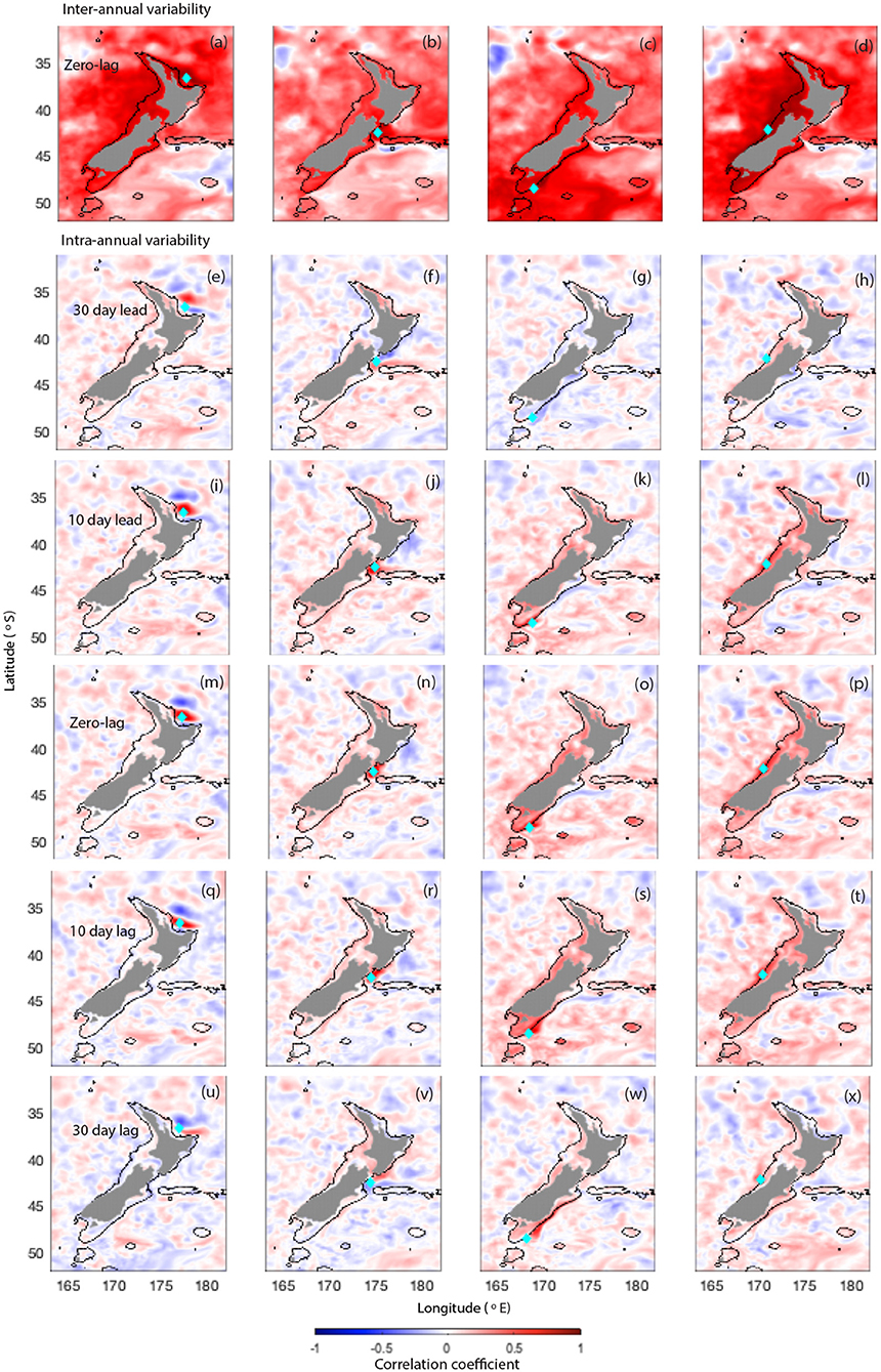
Figure 2. Correlation of UOHC at a given point (shown by turquoise diamond) to UOHC across domain for inter-annual periods at zero-lag (a–d) and intra-annual periods at 30 day lead (e–h), 10 day lead (i–l), zero-lag (m–p), 10 day lag (q–t), and 30 day lag (u–x). The points are in regions (from left to right) 1. Bay of Plenty, 2. Kaikoura, 3. Stewart Plateau and Snares Shelf 4. Hokitika. The 400 m bathymetry contour is shown.
At intra-annual periods the spatial correlations of UOHC reveal the local circulation patterns (Figures 2m–p). In Region 1 (Bay of Plenty), significant correlations (p < 0.05) show an eddy type structure that moves into the region from the north (Figures 2e,i), with heat leaving the bay to the east (Figures 2q,u). In Region 2 (Kaikoura), significant correlations (p < 0.05) imply that heat enters from the east with a lead time of 30 days (Figures 2f,j) and then moves northward along the southeast coast of the North Island (Figures 2r,v). In Region 3 (Stewart Plateau and Snares Shelf region) significant correlations (p < 0.05) exist over a wider region of the southern and western continental shelf with a lead time of 10 days (Figure 2k), with heat then flowing into the Southland Current (Figures 2s,w). Similarly, at Hokitika significant correlations (p < 0.05) with a lead time of 10 days are seen over the continental shelf region on the west coast of NZ (Figure 2l). Positive correlations over this region persist for 10 days, but not for 30 days (Figure 2x).
Based on UOHC computed daily from the 25-year hindcast, we define MHW events within each model grid cell over the 25-year period using the definition of Hobday et al. (2016), as described in Section 2.2. The total percentage time in a MHW, the number of MHWs and the median MHW duration are shown in Figures 3a–c. While the spatial variability across the region is similar when defining MHWs based on UOHC or SST, using UOHC gives more MHW events with longer durations (not shown). For this study we focus on the four regions and MHW events are characterized for a central point within each region (Figure 3b).
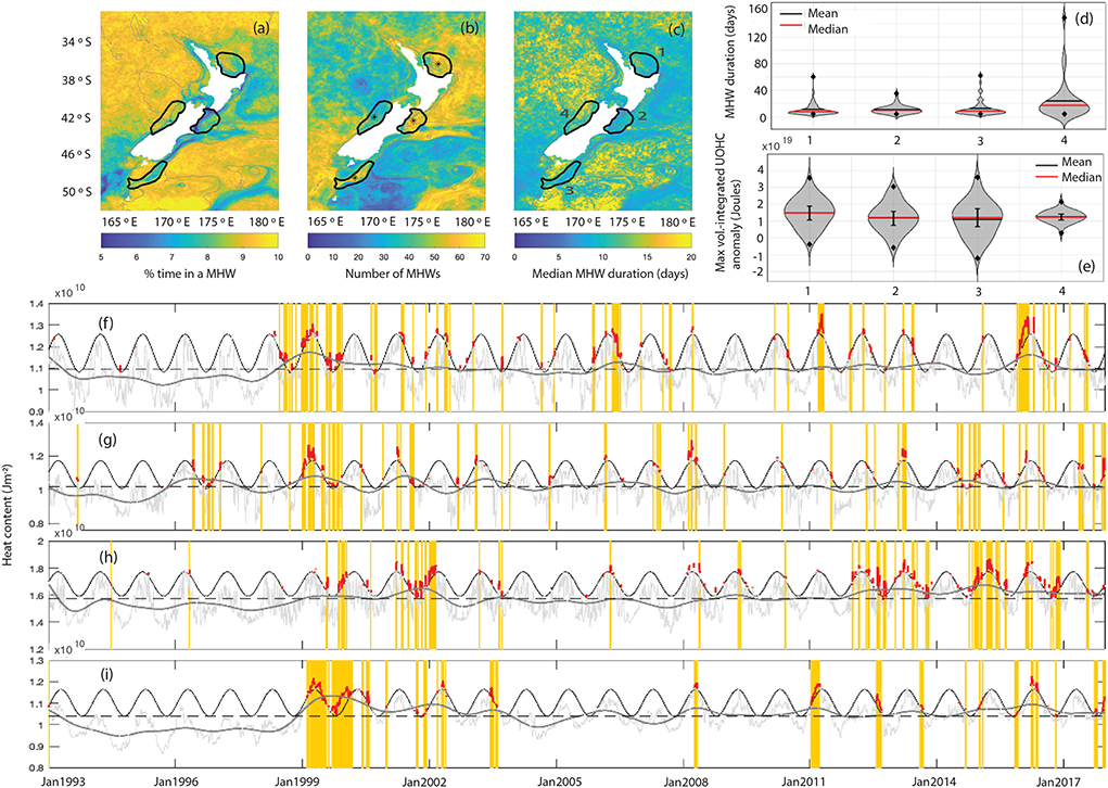
Figure 3. Characterization of MHWs based on UOHC (a–c). Regions for adjoint sensitivity analysis metrics are shown by the black lines: 1. Bay of Plenty, 2. Kaikoura, 3. Stewart Plateau and Snares Shelf 4. Hokitika. Violin plots showing distribution of MHW duration (d) and MHW magnitude (e). Minimum and maximum values are shown by the black diamonds and on (e) error bars showing one standard deviation either side of the median are shown in black. UOHC above the 90th percentile thermocline at central point inside regions 1–4 (f–i) (gray line) and the 90th percentile daily climatological UOHC computed with an 11-day window (black line). The red lines indicate where the UOHC exceeds the 90th percentile daily climatology and the orange regions represent MHW events based on the definition of Hobday et al. (2016), using UOHC rather than SST (that is when the red lines have duration of 5 or more days). The dark gray line shows the heat content low-passed filtered at inter-annual periods.
Over the four regions, we identify 64, 64, 52, and 34 MHWs, respectively, over the 25 years. The median (minimum/maximum) duration of MHWs in days is 8 (5/60), 10 (5/35), 9 (5/62), and 17.5 (5/148) days for regions 1–4, respectively (Figure 3d). MHW magnitude, as defined by the maximum UOHC anomaly (volume-integrated over the defined region, Figure 3e) is greatest in the Region 1 (Bay of Plenty), and similar in the other 3 regions, with considerably lower magnitude variability in Region 4 (Hokitika).
The time series of UOHC display variability at short time-scales (days to weeks) through to inter-annual time scales (Figures 3f–i). For the most part, MHW events often occur during periods when the heat content low-passed filtered at inter-annual periods exceeds the mean, but it is evident from the time series that this is not always the case, and that the short timescale variability is key to tipping the UOHC over the 90th percentile daily climatological value (shown by the red in Figures 3f–i). As such, this study now focuses on identifying and quantifying the processes at play over the onset of the MHW events, focusing on the short timescale processes.
We have shown that the evolution of UOHC on short timescales (days to weeks) appears to be key to initiating MHW events. This variability is embedded in the inter-annual variability, which can be a preconditioner to increasing the likelihood of MHW events, however it is also noted that MHW events can occur outside of these anomalously warm multi-year periods. It is therefore clear that understanding the processes occurring at short temporal and spatial scales is a key to predicting the occurrence of MHW events in regional seas. We now use Adjoint Sensitivity Analysis to focus on the short timescale processes at play over the onset of the MHW events.
We assess the relative sensitivity of UOHC to the prior ocean state and atmospheric forcing over the onset of MHW events. Employing Adjoint Sensitivity Analysis over 5 day periods with the last full day being the first day of the MHW, we investigate the drivers that initialize the MHW. There are 64, 64, 52, and 34 MHWs in Regions 1–4, respectively, so we run a total of 214 5-day adjoint simulations. We perform Adjoint Sensitivity Analysis on UOHC averaged over the given region and over the last day of the 5 day cycle. The cycles are limited to 5 days due to requirement of the linear assumption remaining valid over this length of time, and allow us to investigate the onset of each MHW event over the 5 days prior to the event.
The adjoint sensitivity results are able to reveal the magnitude and the spatial and temporal evolution of the influence that each state variable and forcing field has on the UOHC on the last day of the simulation window. To interpret the adjoint model results, we normalize the sensitivities by an estimate of the typical variability of the corresponding state variable or forcing field value over a 5-day period. The scaled sensitivity is then given by,
where is the output of the adjoint model, Δxi is a perturbation to a model state variable or forcing variable (e.g., temperature, surface wind stress), Nt is the total number of modeled time steps and i is the index of the grid cell of interest. Presenting the scaled sensitivity is useful as the impact of the perturbation of different ocean state variables can be directly compared in units of Joules, and the impact different areas and times can be quantified by summing only over the sensitivities of certain grid cells and times. For example, in Figure 4 we present the scaled sensitivity to temperature over the 5-day window separated by depth (above the mixed layer depth, between the mixed layer and the thermocline, and below the thermocline). We use perturbations, Δxi, based on typical variability of each variable over 5-day periods; we compute the 5-day standard deviations for the 5 days leading up to each MHW event and average them in quadrature.
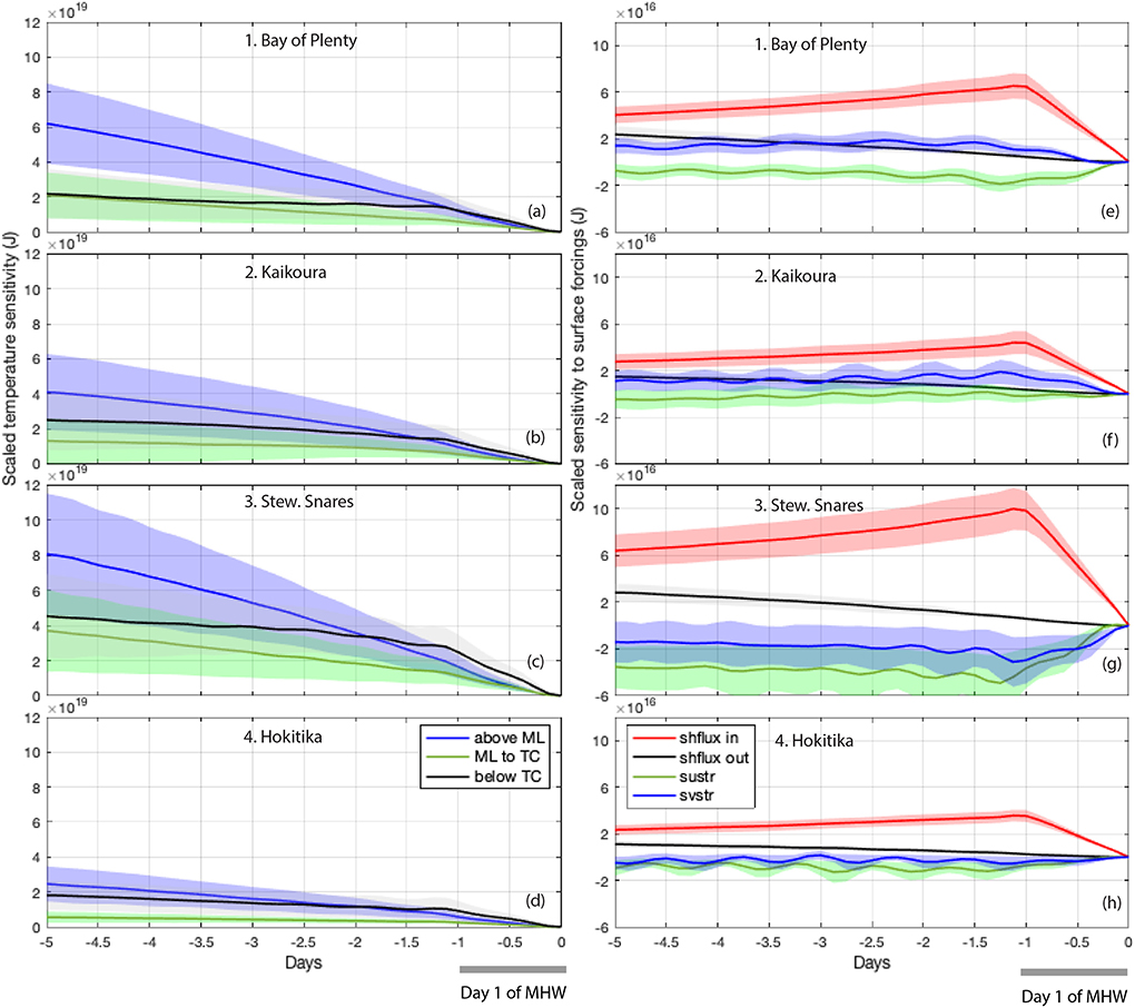
Figure 4. Domain-integrated scaled sensitivities to temperature (left column; a–d) and surface forcings (right column; e–h) over the 5-day adjoint simulations. Temperature sensitivities are for temperature outside of the region and separated by depth and surface heat flux sensitivities are separated into inside and outside of the region. The sensitivities are scaled by the 5-day standard deviations. The magnitudes indicate the amount by which J changes if variable is changed by 1 standard deviation everywhere in the domain for 4 days leading up to the MHW. The magnitudes of J can be compared to those in Figure 3e.
To investigate the dominant drivers of changes to UOHC at the beginning of each MHW event, we present the scaled sensitivities over the 5 day simulation period, with the last day being the first day of each MHW event. Figure 4 shows the mean and standard deviations for all MHW events in each of the four regions. Here, the magnitudes indicate the amount by which J changes if the variable is changed (increased) by one standard deviation everywhere in the summed region. The magnitudes of J can be compared to those in Figure 3e, where the value represents the anomaly above the daily climatology (0.7–2 × 10¹⁹ J), and the total volume integrated heat content values range from 2.6 to 5.4 × 10²⁰ J (Figures 6a–d). It should be noted that temperature sensitivities (Figure 4, left panels) are always positive, meaning that positive perturbations in temperature result in an overall positive change (increase) in UOHC. Likewise, increases in surface heat flux always results in overall increases in UOHC, while positive perturbations to wind stress forcing can result in increases or decreases in overall UOHC (Figure 4, right panels).
For the model variables we compute the sensitivity to changes outside the chosen region, therefore representing how these changes influence UOHC inside the region (for example advection of temperature into the region). As we are interested in the full depth structure of heat transport the temperature sensitivities are computed separately for temperature in the mixed layer, between the mixed layer and the thermocline, and below the thermocline (Figures 4a–d). Scaled sensitivities to other state variables (salt, u, and v) are 1–2 orders of magnitudes smaller than those for temperature and are not shown. Sensitivities to surface heat fluxes are also separated into fluxes directly over the region, and fluxes outside the region (Figures 4e–h).
Changes to temperature in the mixed layer dominates for Region 1 (Bay of Plenty), Region 2 (Kaikoura) and Region 3 (Stewart Plateau/Snares shelf). In the mixed layer, sensitivities increase steadily over the 5 days indicating advection of heat, while below the thermocline the sensitivities remain fairly constant over the 4 days leading up to the first day of the MHW, indicating adjustments at depth on longer timescales. In Region 4 (Hokitika), where currents are typically weak, changes in temperature below the thermocline result in UOHC changes of similar magnitude to advection in the mixed layer. In each case the mixed layer depth and thermocline depth used is averaged over the 5 day adjoint simulation. Mean mixed layer depths (mixed layer depth standard deviation) over all MHW events for Regions 1–4 are 70 m (39 m), 88 m (70 m), 97 m (82 m), 58 m (39 m). Mean thermocline depths (thermocline depth standard deviation) for Regions 1–4 are 106 m (42 m), 115 m (61 m), 192 m (120 m), 104 m (64 m). The perturbations to temperature are shown in Figure 5e.
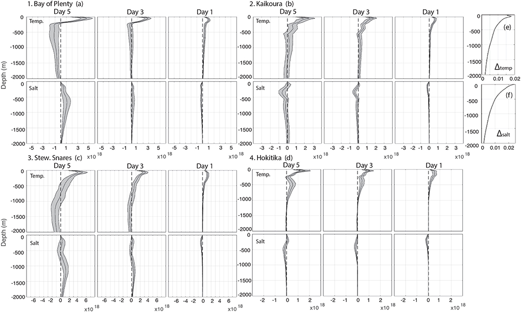
Figure 5. Sensitivity to temperature and salinity outside of the region scaled by the 5-day standard deviations for all MHWs for days 5, 3 and 1 prior to the first day of the MHW event for regions 1. Bay of Plenty (a), 2. Kaikoura (b), 3. Stewart Plateau and Snares Shelf (c), and 4. Hokitika (d). The perturbations used for scaling the sensitivities are shown in (e) for temperature and (f) for salinity.
Surface heat flux perturbations directly over the region have an increasing effect from days −5 to −1 on UOHC on the last day of the simulation window (day −1 to 0), while surface heat flux sensitivities outside of the region gradually decrease (similar to temperature advection in the mixed layer). Indeed the spatial structure of surface heat flux sensitivities follows that of temperature in the mixed layer, representing the advective flow structure. Likewise, for Regions 1–3 the spatial structure of the wind stress sensitivities are consistent with the near-surface advective flow structure indicating that the winds are mostly influencing the surface currents in these regions. In contrast, in Region 4 the wind stress sensitivities show are more widespread spatial influence, described in Section 5.4. Perturbations to net surface heat flux are of the order of 180–200 Wm−2 and perturbations to surface wind stress correspond to changes in wind speed of 6–8 ms−1.
The results show that changes in UOHC are most sensitive to temperature changes outside of the four regions rather than surface fluxes or wind forcing. Advection is described by the sensitivity to changes in advected water mass properties outside of the region over which UOHC is averaged. Sensitivity to advected temperature in the mixed layer is 2–3 orders of magnitude greater than sensitivity to surface heat flux (Figure 4). Since we use an ocean-only model, sensitivities to atmospheric forcing are relative to the imposed surface forcing, as opposed to a dynamic air-sea coupling. Our results show that changes in temperature (typical of 5-day variability) result in greater UOHC changes than changes to surface heat flux (given typical 5-day variability). Temperature changes in the ocean on 5-day timescales are driven by a variety of processes including advection by ocean currents and subduction due to density changes or wind forcing, while surface heat flux changes over 5-days do relatively little to influence UOHC. This result is given that the UOHC is computed for the 90th percentile thermocline depth; the spatial mean depths in Regions 1–4 are 170, 210, 400, and 200 m, respectively. If the depths were shallower, or SST was used as a metric, surface fluxes may be more impactful, e.g., (Elzahaby et al., 2022). Furthermore, the dominance of advection over surface forcings is given that this study focusses on processes that occur over short time scales (5 days). Indeed, surface heat flux and wind forcing changes are likely drivers of UOHC variability over large spatial and temporal scales, causing the inter-annual variability (Figures 2a–d) that acts as a preconditioner to the onset of MHW events (Figures 3f–i).
The subsurface structure of UOHC scaled sensitivities is further investigated in this section. Profiles of sensitivity to temperature and salinity outside of the region for day 5, 3, and 1 prior to the first day of the MHW event reveal the subsurface structure of the sensitivities (Figure 5). Across all regions, sensitivities to temperature outside of the region are positive over the depth range over which UOHC in computed (170– 400 m), while below this depth temperature and salinity have opposing influences representing sensitivities to density changes below the thermocline. As discussed above, this demonstrates two separate mechanisms that influence UOHC; (1) advection of temperature, which occurs predominantly in the upper ocean, and (2) adjustments due to changes in density structure, driving deeper convection. The perturbations to temperature and salinity are shown in Figures 5e,f, respectively.
In Region 1, sensitivities to temperature in the upper 200 m dominate with increases in temperature at these depths resulting in increased UOHC. Below the thermocline, cooler temperature and higher salinity results in increases in UOHC resulting from changes in the density structure below the thermocline. Increased density below 200 m, 5 and 3 days prior to the MHW event results increased UOHC. In Region 2, positive sensitivities to temperature exist in the upper 500 m with highest sensitivities in the upper 200 m (above the thermocline). Reduced density between 200 and 500 m results in higher UOHC, in contrast to Region 1. In Region 3, positive sensitivities to temperature exist over the upper 500 m, with increased in density at depth (below ~700 m) resulting in increased UOHC. In Region 4, the sensitivity profile to temperature is bimodal with positive sensitivities to temperature above 200 m and between 200 and 1,000 m for 5 and 3 days prior to the event, and salinity playing a small role down to 1,000 m. In each region, on day 1 (the first day of the MHW event), sensitivities to temperature exists in the upper 200 m and density changes at depth can have little influence.
The maximum volume-integrated heat content associated with each MHW event (describing the event's magnitude), is inversely related to the thermocline depth (Figures 6a–d). Composites of the high (red) and low (blue) magnitude MHW events show that high magnitude events in regions 1–3 are typically associated with higher sensitivities to temperature in the upper 50–80 m, while lower magnitude events have sensitivities spread over the upper ~150 m corresponding to the deeper mixed layer and thermocline (Figure 6). In Region 4, the high magnitude events also have greater sensitivities to temperature below the thermocline to 1,000 m depth, indicating the influence of density changes at depth on MHWs in this region.
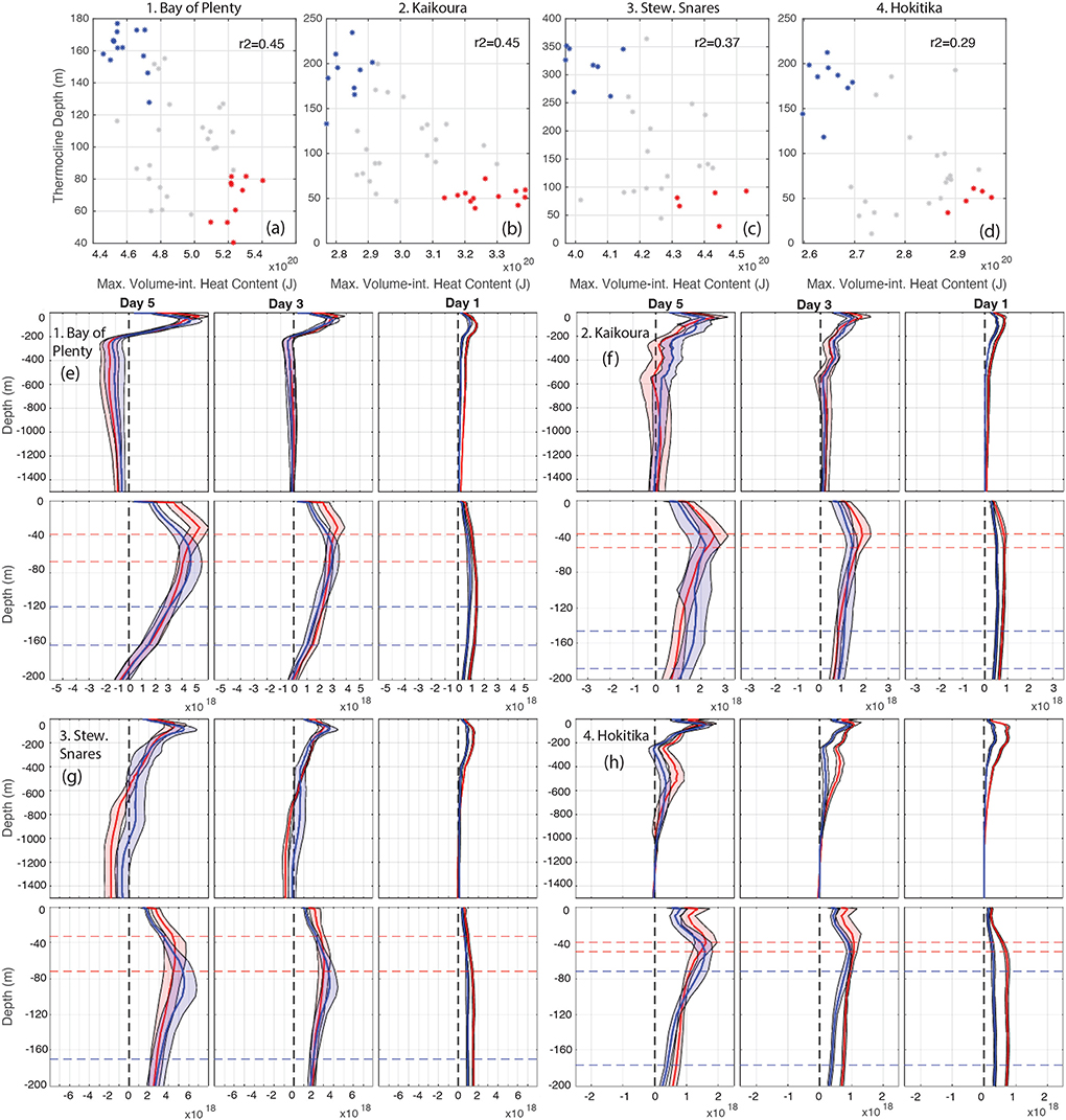
Figure 6. MHW magnitude versus mean thermocline depth over each of the regions and over the 5 days (a–d). MHWs are clustered into mag>65th %tile and TD < 35th %tile (red) and mag <35th %tile and TD>65th %tile (blue). These clusters are used for the composite profiles (e–h). Profiles show the sensitivity to temperature outside of the region scaled by the 5-day standard deviations for composites of high and low magnitude MHWs down to 1500 m (top) and zoomed in to the upper 200 m (bottom), for days 5, 3 and 1 prior to the first day of the MHW event.
Given the dominant influence of changes in temperature in the mixed layer, and changes in temperature and salinity below 200 m, outside of the regions elucidated from the adjoint sensitivity results, we examine the flow structures associated with the onset of MHW events. As each of the four regions experience MHWs at different times and present different circulation dynamics, we consider each region separately. We consider ensembles of the background flow (Figures 7, 9, 11, 13) and adjoint sensitivities (Figures 8, 10, 12, 14) averaged over the 4 days leading up to all MHW events.
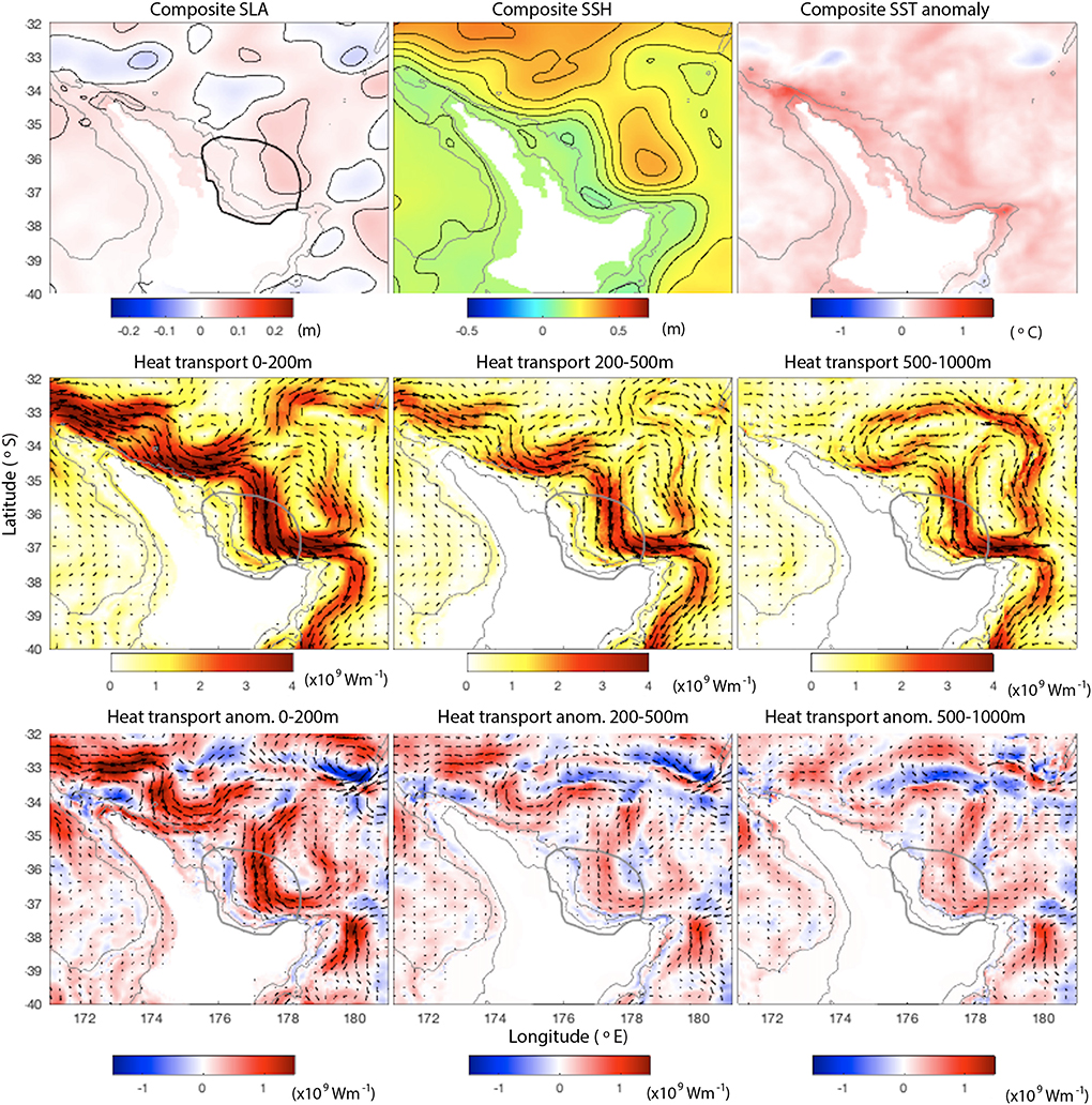
Figure 7. (Top): Ensemble means of SSH anomaly, SSH and SST anomaly averaged over the 4 days leading up to all 64 MHW events in the Bay of Plenty. (Middle): Ensemble means of depth-integrated heat transport averaged over the 4 days leading up to MHW events from 0 to 200, 200 to 500, and 500 to 1,000 m (Wm−1). (Bottom): Ensemble means of depth-integrated heat transport anomalies (Wm−1). Gray lines show the 100 and 1,000 m bathymetry contours.
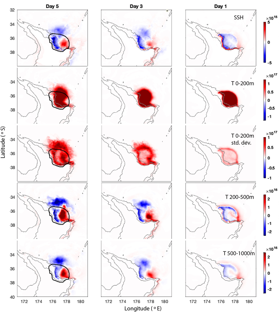
Figure 8. Ensemble sensitivities for days 5, 3, and 1 leading up to all 64 MHW events in the Bay of Plenty. (Top to bottom): Mean scaled sensitivity to SSH, mean scaled sensitivity to temperature from 0 to 200 m, standard deviation of scaled sensitivity to temperature from 0 to 200 m, mean scaled sensitivity to temperature from 200 to 500 m and mean scaled sensitivity to temperature from 500 to 1,000 m. Sensitivities are scaled by the 5-day standard deviations for the days leading up to the MHWs, averaged in quadrature. Gray lines show the 100 and 1,000 m bathymetry contours.
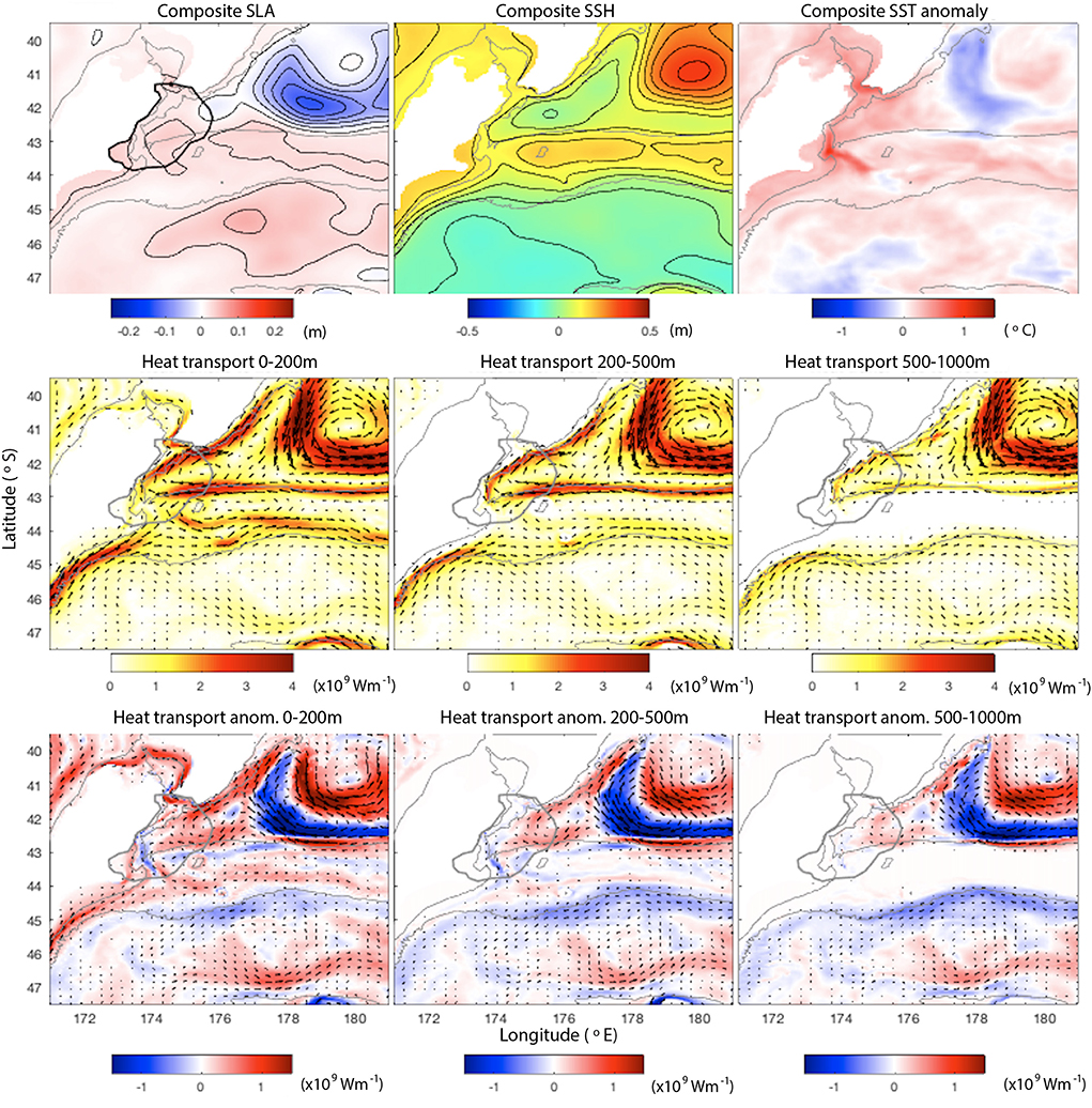
Figure 9. (Top): Ensemble means of SSH anomaly, SSH and SST anomaly averaged over the 4 days leading up to all 64 MHW events in the Kaikoura region. (Middle): Ensemble means of depth-integrated heat transport averaged over the 4 days leading up to MHW events from 0 to 200, 200 to 500, and 500 to 1,000 m (Wm−1). (Bottom): Ensemble means of depth-integrated heat transport anomalies (Wm−1). Gray lines show the 100 and 1,000 m bathymetry contours.
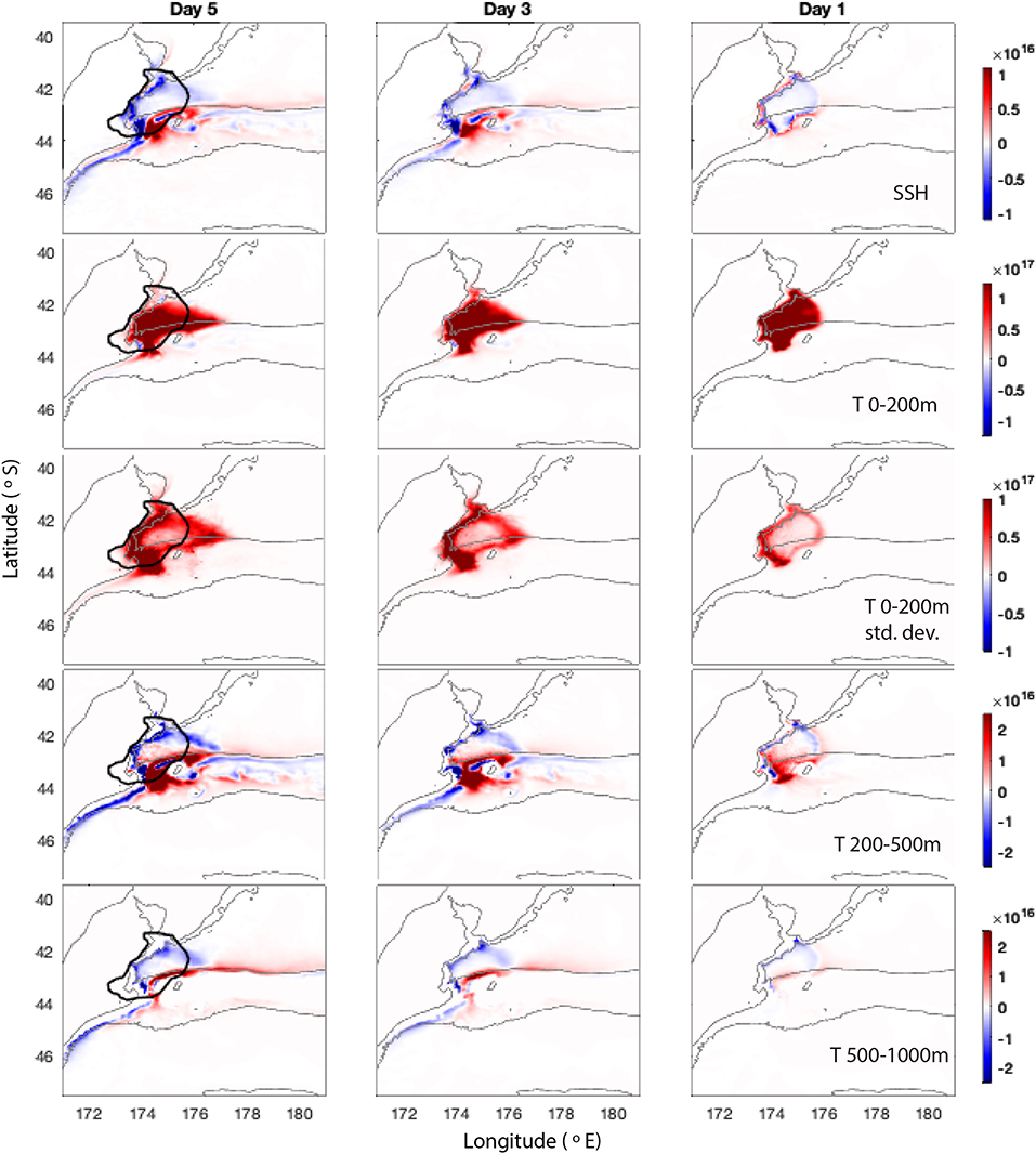
Figure 10. Ensemble sensitivities for days 5, 3, and 1 leading up to all 64 MHW events in the Kaikoura region. (Top to bottom): Mean scaled sensitivity to SSH, mean scaled sensitivity to temperature from 0 to 200 m, standard deviation of scaled sensitivity to temperature from 0 to 200 m, mean scaled sensitivity to temperature from 200 to 500 m and mean scaled sensitivity to temperature from 500 to 1,000 m. Sensitivities are scaled by the 5-day standard deviations for the days leading up to the MHWs, averaged in quadrature. Gray lines show the 100 and 1,000 m bathymetry contours.
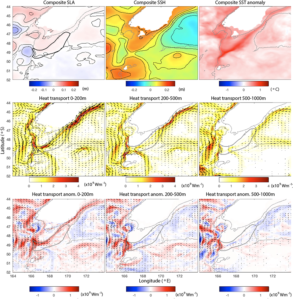
Figure 11. (Top): Ensemble means of SSH anomaly, SSH and SST anomaly averaged over the 4 days leading up to all 52 MHW events in the Stewart Plateau and Snares Shelf region. (Middle): Ensemble means of depth-integrated heat transport averaged over the 4 days leading up to MHW events from 0 to 200, 200 to 500, and 500 to 1,000 m (Wm−1). (Bottom): Ensemble means of depth-integrated heat transport anomalies (Wm−1). Gray lines show the 100 and 1,000 m bathymetry contours.
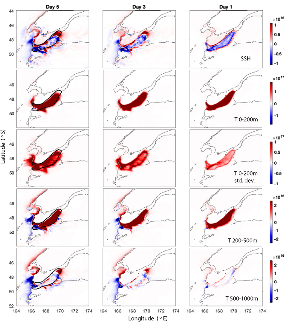
Figure 12. Ensemble sensitivities for days 5, 3, and 1 leading up to all 52 MHW events in the Stewart Plateau and Snares Shelf region. (Top to bottom): Mean scaled sensitivity to SSH, mean scaled sensitivity to temperature from 0 to 200 m, standard deviation of scaled sensitivity to temperature from 0 to 200 m, mean scaled sensitivity to temperature from 200 to 500 m and mean scaled sensitivity to temperature from 500 to 1,000 m. Sensitivities are scaled by the 5-day standard deviations for the days leading up to the MHWs, averaged in quadrature. Gray lines show the 100 and 1,000 m bathymetry contours.
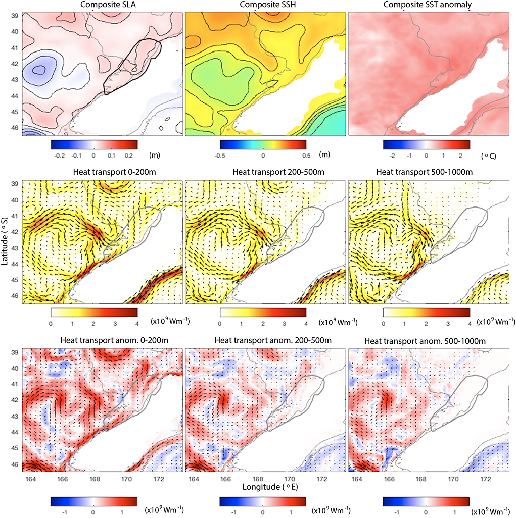
Figure 13. (Top): Ensemble means of SSH anomaly, SSH and SST anomaly averaged over the 4 days leading up to all 34 MHW events in the Hokitika region. (Middle): Ensemble means of depth-integrated heat transport averaged over the 4 days leading up to MHW events from 0 to 200, 200 to 500, and 500 to 1,000 m (Wm−1). (Bottom): Ensemble means of depth-integrated heat transport anomalies (Wm−1). Gray lines show the 100 and 1,000 m bathymetry contours.
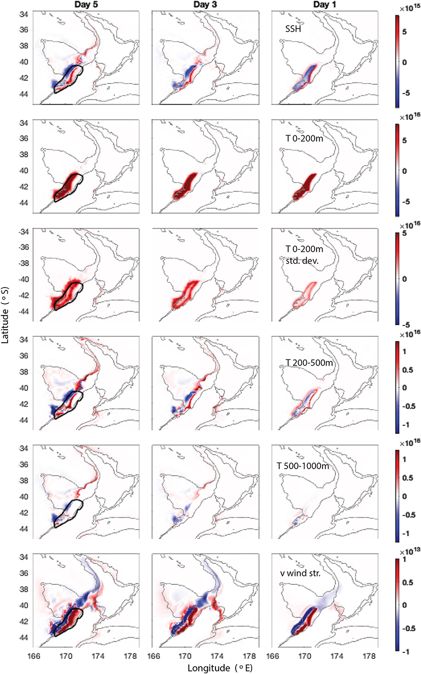
Figure 14. Ensemble sensitivities for days 5, 3, and 1 leading up to all 34 MHW events in the Hokitika region. (Top to bottom) Mean scaled sensitivity to SSH, mean scaled sensitivity to temperature from 0 to 200 m, standard deviation of scaled sensitivity to temperature from 0 to 200 m, mean scaled sensitivity to temperature from 200 to 500 m, mean scaled sensitivity to temperature from 500 to 1,000 m, and mean scaled sensitivity to surface meridional wind stress. Sensitivities are scaled by the 5-day standard deviations for the days leading up to the MHWs, averaged in quadrature. Gray lines show the 100 and 1,000 m bathymetry contours.
We show ensemble means of SSH anomaly, SSH, and SST anomaly (Figures 7, 9, 11, 13 top panels). To understand how the flow structures relate to the onset of MHW events, we compute the vertically-integrated heat transport for the 4 days leading up to each MHW event (for depths 0–200, 200–500, 500–1,000 m). Depth-integrated heat transport from a depth −z1 to −z2 is a vector given by
where Cp is the specific heat of sea water (J(kgK)−1). The ensemble means of vertically-integrated heat transport (Figures 7, 9, 11, 13 middle panels) and vertically-integrated heat transport anomalies relative to the 25-year mean (Figures 7, 9, 11, 13 bottom panels), averaged, averaged over the 4 days leading up the MHW events, reveal the subsurface structure of the heat advection. For the adjoint sensitivities, we present the mean scaled sensitivity (Equation 8) to SSH, mean scaled sensitivity to temperature from 0 to 200 m, standard deviation of scaled sensitivity to temperature from 0 to 200 m, mean scaled sensitivity to temperature from 200 to 500 m and mean scaled sensitivity to temperature from 500 to 1,000 m for days 5, 3, 1 leading up to all MHW events. These are shown in Figures 8, 10, 12, 14 for each of the four regions. As previously the sensitivities are scaled by the 5-day standard deviations for the days leading up to the MHWs, averaged in quadrature, and then summed across the relevant depth-integral.
For the Bay of Plenty, we see a negative SSH anomaly off the northern tip of the North Island, associated with less separation of the EAUC at North Cape, and an eddy dipole directly to the north of the Bay of Plenty, which pumps warm water into the Bay of Plenty region (Figure 7). The SSH sensitivities are consistent with the existence of this eddy dipole to the north of the region and the temperature sensitivities in the upper 200 m reveal that heat is advected into the Bay of Plenty from the north (Figure 8). This reinforces the idea that, rather than separating into the North Cape Eddy, the EAUC pumps warm water from the north into the Bay of Plenty. SST is higher than normal across the entire northern region when MHW events occur in the Bay of Plenty, consistent with Figure 3f where we see that the majority of MHWs occur over multi-year periods when UOHC is anomalously high. Importantly, our results show the importance of the EAUC flow and its associated eddies on initiation of MHWs within these multi-year periods. These results reveal the causal mechanism behind what was suggested by the correlation plots in Figure 2 and described in Section 3.1.
Warmer temperatures at depth (below 200 m) to the east of the Bay of Plenty region up to 5 days prior to the MHW result in increased UOHC in the Bay of Plenty, while cooler temperatures below 200 m to the west and north of the region result in higher UOHC. As salinity shows the opposite pattern (not shown), this is related to the influence of the density structure below the thermocline. The spatial structure of SSH sensitivities is also consistent with this inferred circulation pattern that drives the onset of UOHC extremes in the region.
For Kaikoura, MHW events are associated with a weaker than normal eastward flow as the East Cape Current (ECC) separates and flows eastward, and a stronger westward countercurrent along the Chatham Rise [also resulting in stronger heat transport in the Wairarapa Coastal Current (WCC)]. This flow scenario likely results in heat convergence in the Kaikoura region, causing UOHC extremes. SST is cooler than normal in the ECC and warmer than normal off the east coast of central NZ. Heat is advected into the region from the east in the upper 500 m and from the south, associated with the Southland Current (SC), in the upper 200 m (Figure 9). This advection of temperature from the east and south is demonstrated by the temperature sensitivities in the upper 200 m (Figure 10).
Between 200 and 500 m, and to a lesser extent below 500 m, cooler temperatures against the continental shelf, and warmer temperatures along the Chatham Rise over the 5 days prior to the MHW event result in higher UOHC in the region (Figure 10). As in Region 1, similar spatial structures of the SSH sensitivities and the sensitivities to temperature below 200 m emphasize the importance of the ocean density structure in driving increased heat transport from the east along the northern edge of the Chatham Rise.
The current structure around the Stewart Plateau and Snares Shelf region is particularly complex. In the flow ensemble means (Figure 11), heat transport in the Fiordland Current is reinforced by a low sea level anomaly off the southwestern tip of NZ's South Island. This anomalously warm water hugs the continental shelf around the southern tip of NZ over the upper 200 m feeding warm water into Region 3. SST is broadly higher than normal across the southern region when MHW events occur in the Stewart Plateau and Snares Shelf region, consistent with Figure 3h where we see that the majority of MHWs occur over multi-year periods when UOHC is anomalously high.
The complexities in the current structure are revealed by the SSH sensitivities (Figure 12). Advection into the region from the north is revealed by the temperature sensitivities in the upper 200 m (Figure 12) which also reveal some heat is entering from the south of the region (via the Subantarctic Front). Sensitivities to temperature below 200 m relate to the influence of the density structure on UOHC (Figure 12), with salinity sensitivities at depth having the opposite sign (not shown). Temperature sensitivities below 200 m and sensitivities to SSH extend along the continental shelf on the west coast of the South Island, indicating the wide-spread influence of density structure below 200 m on UOHC in Region 3. This influence in more pronounced in Region 4 and is discussed in the following section.
The correlations with 30-, 10- and 0-day lead times for Region 3 (Figure 2) show no clear flow structure, indicating that the heating occurs due to large scale adjustments at depth on the west coast. The adjoint sensitivity results (Figures 4c, 12) and ensemble mean heat transports (Figure 11) reveal that advection in the Fiordland Current (FC) is important for UOHC in Region 3, and the lagged spatial correlations for UOHC (Figures 2s,w) reveal that heat from Region 3 is then advected in the Southland Current (SC).
MHW events at Hokitika are associated with a broad onshore flow associated with the Subtropical Front that impinges on the west coast of the South Island and warmer than normal SST across the oceanic region west of the South Island (Figure 13). This broad scale SST anomaly when MHW events occur in the Hokitika region is consistent with Figure 3i where we see that almost all of MHWs occur over multi-year periods when UOHC is anomalously high. Anomalously high heat transport occurs over the (5-day) onset of MHW events from the west down to 1,000 m and from the north along the shelf above 500 m (Figure 13).
Temperature sensitivities above 200 m reveal very little advective flow structure, consistent with Figure 4d where advection in the mixed layer was relatively small (compared to the other regions, Figures 4a–c). Some advection is seen into the southwest of the region in the upper 200 m (Figure 14), while the temperature sensitivities below 200 m relate to sensitivities to density changes. Five days prior to the MHW events, Figure 5 shows sensitivity to temperature with depth (outside of the region) is bimodal with a peak in the upper 200 m and a peak at ~500 m. This peak at depth disappears 1 day before the events when sensitivities in the upper 200 m dominate. Temperature sensitivities between 200 and 500 m (Figure 14) reveal that leading up to MHW events cooler (denser) water offshore of the shelf and warmer (less dense) water on the shelf slope leads to an increase in UOHC in the region, suggesting a downwelling process. Indeed in Figure 2 there is no clear flow structure evident in the spatial plots of UOHC correlations at Region 4 (Hokitika), in contrast to Regions 1 and 2, consistent with the downwelling mechanism rather than horizontally dominated flows.
The spatial structure of the surface wind stress sensitivities in Region 4 show wide-spread wind stress sensitivities (Figure 14) indicating that the winds over the west coast of NZ are setting up a downwelling circulation pattern that drives extreme UOHC events in the region. This is consistent with the sensitivities of UOHC to density changes at depth. This is in contrast to the spatial structure of the surface wind stress sensitivities Regions 1–3 (not shown) which simply reveal the local advective flow structure.
We have shown that, embedded in the large scale inter-annual variability of ocean heat content, extremes in upper ocean heat content around NZ are largely driven by processes that occur on short timescales (days to weeks) associated with the local circulation, rather than surface heat fluxes. Regions 1–3 show high sensitivities to temperature in the mixed layer that gradually decrease with time over the onset of the MHW (Figures 4a–c), indicating that advection of temperature in the mixed layer is the dominant driver of the extreme UOHC events. In contrast, in Region 4 where currents are typically weak (Figure 1a), changes in temperature below the thermocline and those in the mixed layer influence UOHC by a similar magnitude (Figure 4d). Regions 1–3 are characterized by having many, short duration MHWs, while Region 4 has fewer, longer duration MHWs (Figures 3d,e). These two regimes correspond to MHWs driven by advection in the mixed layer (Regions 1–3) and MHWs influenced by temperature perturbations above and below the ML in a region characterized by weaker currents (Region 4).
Across all regions, the effects of changes to temperature and salinty below the thermocline on UOHC relate to density changes, indicated by the opposing affects of temperature and salinity (Figure 5), which influence heat convergence into the regions. Using an adjoint model to study sensitivities of ocean heat content in the Labrador Sea, Jones et al. (2018) separate the effects of changes in potential temperature at constant density and changes in density. Similar to our results in the mixed layer for Regions 1–3, they show that sensitivities of heat content to potential temperature reveal the circulation patterns (or advective flow structure). Sensitivities to changes in density were able to reveal regions in which density changes can alter circulation and ultimately influence heat convergence.
Analyzing the four-dimensional structure of the adjoint sensitivities reveals the significance of changes to subsurface temperature (and to a lesser extent, salinity) to UOHC extremes. Mixed layer heat budgets are frequently used to diagnose the drivers of surface warming associated with MHWs (e.g., Elzahaby et al., 2021, 2022); however, the influence of salinity and subsurface water mass properties are often overlooked (Holbrook et al., 2020) yet have been shown to be significant for MHW evolution and persistence (Scannell et al., 2020; Hu et al., 2021). We show that adjustments relating to changes in density structure (well below the mixed layer) are particularly important for MHWs in regions where surface currents (and therefore heat advection) are weak (such as the west coast of NZ). While this study focused on the short-term drivers of UOHC extremes, inter-annual variability and long-term trends in UOHC would also benefit from analysis of the role of subsurface temperature and salinity to better understand the ocean's role in the persistence and evolution of long-lived events.
We show that higher magnitude MHW events are typically associated with shallower mixed layer and thermocline depths, with higher sensitivity to temperature changes in the upper 50–80 m. These results show that, for the same change in temperature, shallower mixed layers result in greater changes in UOHC due to advection of temperature into the region. As noted by Holbrook et al. (2020), when mixed layers are shallower than normal they will warm more quickly for a given input of heat. The influence of density changes at depth were also illuminated by Scannell et al. (2020) who describe the onset of a MHW event during which an increase in stratification likely contributed to the confinement of warm anomalies to the near-surface, enhancing the MHW's intensity.
The flow structures associated with MHW event onset are revealed by the spatial plots of sensitivity to temperature in the upper 200 m, for Regions 1–3, with the sensitivities of the ensembles (Figures 8, 10, 12) revealing the source of advected temperature consistent with the ensemble mean flow structures (Figures 7, 9, 11). The spatial structure of the surface wind stress sensitivities in Regions 1–3 reveal the local advective flow structure, while the wide-spread wind stress sensitivities in Region 4 (Figure 14) indicate a downwelling mechanism over the west coast of NZ driving extreme UOHC events. This is consistent with findings by Jones et al. (2018) who show significant positive alongshore wind stress sensitivity patterns that largely reinforce the adjustment pathways for heat content in a region of deep convection. The spatial correlation of UOHC at intra-annual periods (Figure 2) reveal these large scale adjustments over the west coast, in contrast to the correlations in Regions 1 and 2 revealing the advective flow structure.
MHW predictability will be more or less challenging depending on the regions and drivers (Jacox et al., 2019; Holbrook et al., 2020) and an understanding of the temporal and spatial scales of variability and the associated physical drivers of heat content extremes is key to developing effective prediction systems. Here, we emphasize the different timescales associated with UOHC variability (Figures 1c,d, 2, 3f–i). On short timescales (days to weeks), the local circulation drives changes either through mesoscale eddy and boundary current driven transport (Region 1 and 2), large scale density adjustments driving deep circulation changes (Region 4), or a combination of the two (Region 3) (Figures 2, 7–14). Understanding the prevailing short-term drivers associated with heat content extremes is an important step toward accurate MHW predictability on intra-annual time scales, allowing the prediction of short-lived MHW events within the longer term (inter-annual) heat content variability.
The use of the adjoint model provides direct connections to the dynamical drivers of UOHC extremes, therefore explaining the fundamental dynamics of back-trajectory teleconnections. This is in contrast to other studies that use concurrent correlations which are unable to imply causation. In addition, the adjoint sensitivity fields may also be used to inform the design of future observational networks (e.g., Heimbach et al., 2011; Loose et al., 2020). For instance, on the north and east coasts of NZ focus should be given to observations that will improve predictions of the boundary current circulation and associated eddies, while on the west coast, monitoring of temperature and salinity changes along the continental slope to 1,000 m would be useful in improving model predictions of MHWs. Future changes to UOHC under climate change can also be implied from the adjoint model results given the knowledge of the processes that control UOHC on both regional and local scales, as discussed in Hahn-Woernle et al. (2020).
Our results show a clear temporal scale separation in UOHC variability in oceanic regions around NZ. UOHC at the four near-coast locations shows large scale positive correlation with UOHC over the entire NZ region at inter-annual scales with temporal decorrelation scales of 3–5 years. At intra-annual (60–250 days) scales, spatial correlations relate to local processes and have temporal decorrelation scales of 30 days. While MHW events occur most often during the multi-year periods where UOHC is anomalously high over a broad region, the onset of MHW events in the near-coast regions is driven by local processes on timescales of days to weeks.
Using Adjoint Sensitivity Analysis we revealed that advection of temperature in the mixed layer is the dominant driver of UOHC extremes along the north and east coasts of NZ. Here, changes in UOHC were most sensitive to changes in temperature in the mixed layer outside of the chosen regions, rather than changes in surface forcings. On the west coast, advection is less important and UOHC changes are driven by changes in the density structure in the upper 1,000 m set up by downwelling winds. The spatial structure of the adjoint sensitivities revealed the origins of the adjective heat fluxes above 200 m and the importance of density structure below the thermocline (~200 m). We find common flow structures associated with the onset of MHW events which show heat transport anomalies consistent with the structure of temperature advection revealed by the adjoint sensitivity results. Understanding the local circulation dynamics associated with MHW onset is key to prediction of MHW events on short time scales (days to weeks).
The datasets presented in this study can be found in online repositories. The names of the repository accession number(s) can be found below: https://doi.org/10.5281/zenodo.5895265 (Azevedo Correia de Souza, 2022).
The Moana Project was conceived by MR. The free-running Regional Ocean Modeling System model was configured and the simulation performed over the long-term hindcast period by JMACDS. The long-term hindcast model data was analyzed to identify marine heatwave events by CK. The adjoint model simulations were designed, configured, analyzed, and interpreted by CK. The manuscript was written by CK with input from MR. All authors contributed to the scope of the study. All authors contributed to the article and approved the submitted version.
This work was a contribution to the Moana Project (www.moanaproject.org), funded by the New Zealand Ministry of Business Innovation and Employment, contract number METO1801.
We thank Mary Livingston from New Zealand DPI for insight into the regions most useful to the fishing industry.
Author JMACDS is employed by MetOcean Solutions.
The remaining authors declare that the research was conducted in the absence of any commercial or financial relationships that could be construed as a potential conflict of interest.
All claims expressed in this article are solely those of the authors and do not necessarily represent those of their affiliated organizations, or those of the publisher, the editors and the reviewers. Any product that may be evaluated in this article, or claim that may be made by its manufacturer, is not guaranteed or endorsed by the publisher.
Azevedo Correia de Souza, J., Suanda, S. H., Couto, P. P., Smith, R. O., Kerry, C., and Roughan, M. (2022). Moana Ocean Hindcast–a 25+ years simulation for New Zealand Waters using the ROMS v3. 9 model. EGUsphere. p. 1–34. doi: 10.5194/egusphere-2022-41
Behrens, E., Fernandez, D., and Sutton, P. (2019). Meridional oceanic heat transport influences marine heatwaves in the Tasman Sea on interannual to decadal timescales. Front. Mar. Sci. 6, 228. doi: 10.3389/fmars.2019.00228
Benthuysen, J., Feng, M., and Zhong, L. (2014). Spatial patterns of warming off Western Australia during the 2011 Ningaloo Ni no: quantifying impacts of remote and local forcing. Continent. Shelf Res. 91, 232–246. doi: 10.1016/j.csr.2014.09.014
Bowen, M., Markham, J., Sutton, P., Zhang, X., Wu, Q., Shears, N., et al. (2017). Interannual variability of sea surface temperature in the southwest pacific and the role of ocean dynamics. J. Climate 30, 18. doi: 10.1175/JCLI-D-16-0852.1
Changler, M., Bowen, M., and Smith, R. O. (2021). The Fiordland Current, southwest New Zealand: mean, variability, and trends. New Zealand J. Marine Freshwater Res. 55, 156–176. doi: 10.1080/00288330.2019.1629467
Chen, K., Gawarkiewicz, G., Kwon, Y.-O., and Zhang, W. G. (2015). The role of atmospheric forcing versus ocean advection during the extreme warming of the Northeast US continental shelf in 2012. J. Geophys. Res. Oceans 120, 4324–4339. doi: 10.1002/2014JC010547
Chiswell, S. M., Bostock, H. C., Sutton, P. J. H., and Williams, M. J. M. (2015). Physical oceanography of the deep seas around New Zealand: a review. N. Z. J. Mar. Freshw. Res. 49, 286–317. doi: 10.1080/00288330.2014.992918
Chiswell, S. M., and Roemmich, D. (1998). The East Cape Current and two eddies: a mechanism for larval retention? N. Z. J. Mar. Freshw. Res. 32, 385–397. doi: 10.1080/00288330.1998.9516833
Darmaraki, S., Somot, S., Sevault, F., and Nabat, P. (2019a). Past variability of Mediterranean Sea marine heatwaves. Geophys. Res. Lett. 46, 9813–9823. doi: 10.1029/2019GL082933
Darmaraki, S., Somot, S., Sevault, F., Nabat, P., Cabos Narvaez, W. D., Cavicchia, L., et al. (2019b). Future evolution of marine heatwaves in the Mediterranean Sea. Clim. Dyn. 53, 1371–1392. doi: 10.1007/s00382-019-04661-z
de Burgh-Day, C. O., Spillman, C. M., Smith, G., and Stevens, C. L. (2022). Forecasting extreme marine heat events in key aquaculture regions around New Zealand. J. Southern Hemisphere Earth Syst. Sci. 72, 58–72. doi: 10.1071/ES21012
Elzahaby, Y., and Schaeffer, A. (2019). Observational insight into the subsurface anomalies of marine heatwaves. Front. Mar. Sci. 6, 745. doi: 10.3389/fmars.2019.00745
Elzahaby, Y., Schaeffer, A., Roughan, M., and Delaux, S. (2022). Why the mixed layer depth matters when diagnosing marine heatwave drivers using a heat budget approach. Front. Clim. 4, 838017. doi: 10.3389/fclim.2022.838017
Elzhaby, Y., Schaeffer, A., Roughan, M., and Delaux, S. (2021). Oceanic circulation drives the deepest and longest marine heatwaves in the East Australian Current system. Geophys. Res. Lett. 48, e2021GL094785. doi: 10.1029/2021GL094785
Errico, R. M., and Vukicevic, T. (1991). Sensitivity analysis using an adjoint of the PSU-NCAR mesoscale model. Mon. Weather Rev., 120:1644–1660. doi: 10.1175/1520-0493(1992)120<1644:SAUAAO>2.0.CO;2
Fairall, C. W., Bradley, E. F., Rogers, D. P., Edson, J. B., and Young, G. S. (1996). Bulk parameterization of air-sea fluxes for tropical ocean-global atmosphere Coupled-Ocean Atmosphere Response Experiment. J. Geophys. Res. Oceans 101, 3747–3764. doi: 10.1029/95JC03205
Fernandez, D., Bowen, M., and Sutton, P. (2018). Variability, coherence and forcing mechanisms in the New Zealand ocean boundary currents. Prog. Oceanogr. 165, 168–188. doi: 10.1016/j.pocean.2018.06.002
Fiedler, P. C. (2010). Comparison of objective descriptions of the thermocline. Limnol. Oceanogr. Methods 8, 313–325. doi: 10.4319/lom.2010.8.313
Frölicher, T. L., Fischer, E. M., and Gruber, N. (2018). Marine heatwaves under global warming. Nature 560, 360–364. doi: 10.1038/s41586-018-0383-9
Hahn-Woernle, L., Powell, B., Lundesgaard, Ø., and van Wessem, M. (2020). Sensitivity of the summer upper ocean heat content in a western antarctic peninsula fjord. Prog. Oceanogr. 183, 102287. doi: 10.1016/j.pocean.2020.102287
Heath, R. (1982). What drives the mean circulation on the New Zealand west coast continental shelf? N. Z. J. Mar. Freshw. Res. 16, 215–226. doi: 10.1080/00288330.1982.9515964
Heidemann, H., and Ribbe, J. (2019). Marine heat waves and the influence of El Ni no off southeast Queensland, Australia. Front. Mar. Sci. 6, 56. doi: 10.3389/fmars.2019.00056
Heimbach, P., Wunsch, C., Ponte, R. M., Forget, G., Hill, C., and Utke, J. (2011). Timescales and regions of the sensitivity of Atlantic meridional volume and heat transport: toward observing system design. Deep Sea Res. II Top. Stud. Oceanogr. 58, 1858–1879. doi: 10.1016/j.dsr2.2010.10.065
Hobday, A. J., Alexander, L. V., Perkins, S. E., Smale, D. A., Straub, S. C., Oliver, E. C., et al. (2016). A hierarchical approach to defining marine heatwaves. Prog. Oceanogr. 141, 227–238. doi: 10.1016/j.pocean.2015.12.014
Holbrook, N., Gupta, A., Oliver, E., Hobday, A., Benthuysen, J., Scannell, H., et al. (2020). Keeping pace with marine heatwaves. Nat. Rev. Earth Environ. 1, 482–493. doi: 10.1038/s43017-020-0068-4
Holbrook, N. J., Scannell, H. A., Gupta, A. S., Benthuysen, J. A., Feng, M., Oliver, E. C., et al. (2019). A global assessment of marine heatwaves and their drivers. Nat. Commun. 10, 1–13. doi: 10.1038/s41467-019-10206-z
Hopkins, J., Shaw, A., and Challenor, P. (2010). The Southland front, New Zealand: variability and ENSO correlations. Continent. Shelf Res. 30, 1535–1548. doi: 10.1016/j.csr.2010.05.016
Hu, S., Li, S., Zhang, Y., Guan, C., Du, Y., Feng, M., et al. (2021). Observed strong subsurface marine heatwaves in the tropical western Pacific Ocean. Environ. Res. Lett. 16, 104024. doi: 10.1088/1748-9326/ac26f2
Jackson, J. M., Johnson, G. C., Dosser, H. V., and Ross, T. (2021). Warming from recent marine heatwave lingers in deep British Columbia fjord. Geophys. Res. Lett. 45, 9757–9764. doi: 10.1029/2018GL078971
Jacox, M., Tommasi, D., Alexander, M., Hervieux, G., and Stock, C. (2019). Predicting the evolution of the 2014-16 California Current System marine heatwave from an ensemble of coupled global climate forecasts. Front. Mar. Sci. 6, 497. doi: 10.3389/fmars.2019.00497
Jean-Michel, L., Eric, G., Romain, B.-B., Gilles, G., Angèlique, M., Marie, D., et al. (2021). The copernicus global 1/12 ° oceanic and sea ice GLORYS12 reanalysis. Front. Earth Sci. 9, 698876. doi: 10.3389/feart.2021.698876
Jones, D. C., Forget, G., Sinha, B., Josey, S. A., Boland, E. J., Meijers, A. J., et al. (2018). Local and remote influences on the heat content of the Labrador Sea: an adjoint sensitivity study. J. Geophys. Res. Oceans 123, 2646–2667. doi: 10.1002/2018JC013774
Kerry, C. (2014). Predictability in a region of strong internal tides ad dynamic mesoscale circulation: The Philippine Sea (Ph.D. thesis). School of Ocean and Earth Science, University of Hawaii at Manoa, Honolulu, HI, United States.
Kerry, C., and Roughan, M. (2020). Downstream evolution of the East Australian Current system: Mean flow, seasonal, and intra-annual variability. J. Geophys. Res. Oceans. 125, e2019JC015227. doi: 10.1029/2019JC015227
Kerry, C., Roughan, M., and Azevedo Correia de Souza, J. (2022). Variability of boundary currents and ocean heat content around New Zealand. J. Geophys. Res. Oceans.
Kerry, C. G., and Powell, B. S. (2022). Including tides improves subtidal prediction in a region of strong surface and internal tides and energetic mesoscale circulation. J. Geophys. Res. Oceans 127, e2021JC018314. doi: 10.1029/2021JC018314
Li, J., Roughan, M., and Kerry, C. (2022). Variability and drivers of ocean temperature extremes in a warming western boundary current. J. Clim. 35, 1097–1111. doi: 10.1175/JCLI-D-21-0622.1
Li, Z., Holbrook, N. J., Zhang, X., Oliver, E. C. J., and Cougnon, E. A. (2020). Remote forcing of Tasman Sea marine heatwaves. J. Clim. 33, 5337–5354. doi: 10.1175/JCLI-D-19-0641.1
Loose, N., Heimbach, P., Pillar, H., and Nisancioglu, K. H. (2020). Quantifying dynamical proxy potential through shared adjustment physics in the North Atlantic. J. Geophys. Res. Oceans 125, e2020JC016112. doi: 10.1029/2020JC016112
Matthews, D., Powell, B. S., and Janekovic, I. (2012). Analysis of four-dimensional variational state estimation of the Hawaiian waters. J. Geophys. Res. Oceans 117, C03013. doi: 10.1029/2011JC007575
Moore, A., Arango, H. G., Di Lorenzo, E., Miller, A. J., and Cornuelle, B. D. (2009). An adjoint sensitivity analysis of the southern California current circulation and ecosystem. J. Phys. Oceanogr. 39, 702–720. doi: 10.1175/2008JPO3740.1
Moore, A. M., Arango, H. G., Di Lorenzo, E., Cornuelle, B. D., Miller, A. J., and Neilson, D. J. (2004). A comprehensive ocean prediction and analysis system based on the tangent linear and adjoint of a regional ocean model. Ocean Modell. 7, 227–258. doi: 10.1016/j.ocemod.2003.11.001
Oke, P. R., Pilo, G. S., Ridgway, K. R., Kiss, A., and Rykova, T. (2019a). A search for the Tasman Front. J. Mar. Syst. 199, 103217. doi: 10.1016/j.jmarsys.2019.103217
Oke, P. R., Roughan, M., Cetina-Heredia, P., Pilo, G. S., Ridgway, K. R., Rykova, T., et al. (2019b). Revisiting the circulation of the East Australian Current: its path, separation, and eddy field. Prog. Oceanogr. 176, 102139. doi: 10.1016/j.pocean.2019.102139
Oliver, E. C., Benthuysen, J. A., Bindoff, N. L., Hobday, A. J., Holbrook, N. J., Mundy, C. N., et al. (2017). The unprecedented 2015/16 Tasman Sea marine heatwave. Nat. Commun. 8, 1–12. doi: 10.1038/ncomms16101
Oliver, E. C., Donat, M. G., Burrows, M. T., Moore, P. J., Smale, D. A., Alexander, L. V., et al. (2018a). Longer and more frequent marine heatwaves over the past century. Nat. Commun. 9, 1–12. doi: 10.1038/s41467-018-03732-9
Oliver, E. C., Lago, V., Hobday, A. J., Holbrook, N. J., Ling, S. D., and Mundy, C. N. (2018b). Marine heatwaves off eastern Tasmania: trends, interannual variability, and predictability. Prog. Oceanogr. 161, 116–130. doi: 10.1016/j.pocean.2018.02.007
Perez, E., Ryan, S., Andres, M., Gawarkiewicz, G., Ummenhofer, C., Bane, J., et al. (2021). Understanding physical drivers of the 2015/16 marine heatwaves in the Northwest Atlantic. Sci. Rep. 11, 1–11. doi: 10.1038/s41598-021-97012-0
Powell, B. S., Cornuelle, B. D., and Kerry, C. G. (2013). Using a numerical model to understand the connection between the ocean and travel time measurements. J. Acoust. Soc. Am. 134, 3211–3222. doi: 10.1121/1.4818786
Powell, B. S., Janekovic, I., Carter, G. S., and Merrifield, M. A. (2012). Sensitivity of internal tide generation in Hawaii. Geophys. Res. Lett. 39, 1–6. doi: 10.1029/2012GL051724
Ridgway, K., and Dunn, J. (2003). Mesoscale structure of the mean East Australian Current system and its relationship with topography. Prog. Oceanogr. 56, 189–222. doi: 10.1016/S0079-6611(03)00004-1
Roemmich, D., and Sutton, P. (1998). The mean and variability of ocean circulation past northern New Zealand: Determining the representativeness of hydrographic climatologies. J. Geophys. Res. Oceans 103, 13041–13054. doi: 10.1029/98JC00583
Roquet, F., Madec, G., Brodeau, L., and Nycander, J. (2015). Defining a simplified yet “realistic” equation of state for seawater. J. Phys. Ocean. 45, 2564–2579. doi: 10.1175/JPO-D-15-0080.1
Ryan, S., Ummenhofer, C. C., Gawarkiewicz, G., Wagner, P., Scheinert, M., Biastoch, A., et al. (2021). Depth structure of Ningaloo Ni no/Ni na events and associated drivers. J. Clim. 34, 1767–1788. doi: 10.1175/JCLI-D-19-1020.1
Rykova, T., Oke, P., and Griffin, D. (2017). A comparison of the structure, properties, and water mass composition of quasi-isotropic eddies in Western Boundary Currents in an eddy-resolving ocean model. Ocean Modell. 114, 1–13. doi: 10.1016/j.ocemod.2017.03.013
Scannell, H. A., Johnson, G. C., Thompson, L., Lyman, J. M., and Riser, S. C. (2020). Subsurface evolution and persistence of marine heatwaves in the Northeast Pacific. Geophys. Res. Lett. 47, e2020GL090548. doi: 10.1029/2020GL090548
Schaeffer, A., and Roughan, M. (2017). Subsurface intensification of marine heatwaves off southeastern Australia: the role of stratification and local winds. Geophys. Res. Lett. 44, 5025–5033. doi: 10.1002/2017GL073714
Schlegel, R. W., Oliver, E. C., Perkins-Kirkpatrick, S., Kruger, A., and Smit, A. J. (2017). Predominant atmospheric and oceanic patterns during coastal marine heatwaves. Front. Mar. Sci. 4, 323. doi: 10.3389/fmars.2017.00323
Shchepetkin, A. F., and McWilliams, J. C. (2005). The regional oceanic modeling system (ROMS): a split-explicit, free-surface, topography-following-coordinate oceanic model. Ocean Modell. 9, 347–404. doi: 10.1016/j.ocemod.2004.08.002
Stanton, B. R. (1976). Circulation and hydrology off the west coast of the South Island, New Zealand. N. Z. J. Mar. Freshw. Res. 10, 445–467. doi: 10.1080/00288330.1976.9515629
Stevens, C. L., O'Callaghan, J. M., Chiawekk, S. M., and Hadfueld, M. G. (2021). Physical oceanography of New Zealand/Aotearoa shelf seas- A review. New Zealand J. Marine Freshwater Res. 55, 6–45. doi: 10.1080/00288330.2019.1588746
Sutton, P. J. (2003). The Southland Current: a subantarctic current. N. Z. J. Mar. Freshw. Res. 37, 645–652. doi: 10.1080/00288330.2003.9517195
Sutton, P. J., and Bowen, M. (2019). Ocean temperature change around New Zealand over the last 36 years. N. Z. J. Mar. Freshw. Res. 53, 305–326. doi: 10.1080/00288330.2018.1562945
Tilburg, C. E., Hurlburt, H. E., O'Brien, J. J., and Shriver, J. F. (2001). The dynamics of the East Australian current system: the Tasman front, the East Auckland current, and the East Cape current. J. Phys. Oceangraph. 31, 2917–2943. doi: 10.1175/1520-0485(2001)031<2917:TDOTEA>2.0.CO;2
Veneziani, M., Edwards, C., and Moore, A. (2009). A central California coastal ocean modeling study: 2. Adjoint sensitivities to local and remote forcing mechanisms. J. Geophys. Res. Oceans 114, C4. doi: 10.1029/2008JC004775
Zhan, P., Gopalakrishnan, G., Subramanian, A. C., Guo, D., and Hoteit, I. (2018). Sensitivity studies of the Red Sea eddies using adjoint method. J. Geophys. Res. Oceans 123, 8329–8345. doi: 10.1029/2018JC014531
Zhang, W. G., Wilkin, J. L., Levin, J. C., and Arango, H. G. (2009). An adjoint sensitivity study of buoyancy- and wind-driven circulation on the New Jersey inner shelf. J. Phys. Oceanogr. 39, 1652–1668. doi: 10.1175/2009JPO4050.1
Keywords: marine heatwaves, Tasman Sea, New Zealand, regional, upper ocean heat content, Adjoint Sensitivity Analysis, East Australian Current eastern extension
Citation: Kerry C, Roughan M and Azevedo Correia de Souza JM (2022) Drivers of upper ocean heat content extremes around New Zealand revealed by Adjoint Sensitivity Analysis. Front. Clim. 4:980990. doi: 10.3389/fclim.2022.980990
Received: 29 June 2022; Accepted: 06 October 2022;
Published: 28 October 2022.
Edited by:
Svenja Ryan, Woods Hole Oceanographic Institution, United StatesReviewed by:
Xiaohui Liu, Second Institute of Oceanography, Ministry of Natural Resources, ChinaCopyright © 2022 Kerry, Roughan and Azevedo Correia de Souza. This is an open-access article distributed under the terms of the Creative Commons Attribution License (CC BY). The use, distribution or reproduction in other forums is permitted, provided the original author(s) and the copyright owner(s) are credited and that the original publication in this journal is cited, in accordance with accepted academic practice. No use, distribution or reproduction is permitted which does not comply with these terms.
*Correspondence: Colette Kerry, Yy5rZXJyeUB1bnN3LmVkdS5hdQ==
Disclaimer: All claims expressed in this article are solely those of the authors and do not necessarily represent those of their affiliated organizations, or those of the publisher, the editors and the reviewers. Any product that may be evaluated in this article or claim that may be made by its manufacturer is not guaranteed or endorsed by the publisher.
Research integrity at Frontiers
Learn more about the work of our research integrity team to safeguard the quality of each article we publish.