 Ishrat Jahan Dollan
 Viviana Maggioni
 Jeremy Johnston
 Gustavo de A. Coelho
 James L. Kinter III
- 1Sid and Reva Dewberry Department of Civil, Environmental and Infrastructure Engineering, George Mason University, Fairfax, VA, United States
- 2Department of Atmospheric, Oceanic and Earth Sciences, Center for Ocean-Land-Atmosphere Studies, George Mason University, Fairfax, VA, United States
Global climate models and long-term observational records point to the intensification of extreme precipitation due to global warming. Such intensification has direct implications for worsening floods and damage to life and property. This study investigates the projected trends (2015–2100) in precipitation climatology and daily extremes using Community Earth System Model Version 2 large ensemble (CESM2-LE) simulations at regional and seasonal scales. Specifically, future extreme precipitation is examined in National Climate Assessment (NCA) regions over the Contiguous United States using SSP3-7.0 (Shared Socioeconomic Pathway). Extreme precipitation is analyzed in terms of daily maximum precipitation and simple daily intensity index (SDII) using Mann-Kendall (5% significance level) and Theil-Sen (TS) regression. The most substantial increases occur in the highest precipitation values (95th) during summer and winter clustered in the Midwest and Northeast, respectively, according to long-term extreme trends evaluated in quantiles (i.e., 25, 50, 75, and 95th). Seasonal climatology projections suggest wetting and drying patterns, with wetting in spring and winter in the eastern areas and drying during summer in the Midwest. Lower quantiles in the central U.S. are expected to remain unchanged, transitioning to wetting patterns in the fall due to heavier precipitation. Winter positive trends (at a 5% significance level) are most prevalent in the Northeast and Southeast, with an overall ensemble agreement on such trends. In spring, these trends are predominantly found in the Midwest. In the Northeast and Northern Great Plains, the intensity index shows a consistent wetting pattern in spring, winter, and summer, whereas a drying pattern is projected in the Midwest during summer. Normalized regional changes are a function of indices, quantiles, and seasons. Specifically, seasonal accumulations present larger changes (~30% and above) in summer and lower changes (< ~20%) in winter in the Southern Great Plains and the Southwestern U.S. Examining projections of extreme precipitation change across distinct quantiles provides insights into the projected variability of regional precipitation regimes over the coming decades.
Introduction
Anthropogenic actions that alter the Earth's climate (Solomon et al., 2007) have the potential to cause irreversible disruptions in the twenty-first century. These disruptions are expected to be seasonally and regionally variable and include the potential for large-scale amplification of extreme precipitation events (Pfahl et al., 2017). Agreement persists among climate scientists that copious greenhouse gas emissions contribute to accelerated global-scale warming (Anderson et al., 2016). The Synthesis Report highlights that significant emission reductions are required to limit the global mean surface temperature increase to < 2°C above the pre-industrial level (IPCC, 2014). The increase in temperature, in turn, has a direct link to atmospheric water holding capacity (O'Gorman and Muller, 2010), consequently creating conditions for more intense precipitation events. Several global-scale studies have clarified the connection between the hydrologic cycle and global warming (Trenberth, 1999; Allen and Ingram, 2002; Trenberth et al., 2003). The latest Intergovernmental Panel on Climate Change (IPCC) Assessment Report (AR6) also documents increasingly intense precipitation over most lands (IPCC, 2021). The internal climate variability introduces uncertainties in characterizing the distribution of extremes at regional scales, which requires robust evaluation of large ensembles (Fischer et al., 2013). The present study uses a large ensemble to assess projected seasonal climatology and extremes over the Contiguous United States (CONUS). Future precipitation characteristics are essential for understanding the evolution of the hydrological cycle (Tabari, 2020), adaptive flood engineering design (Madsen et al., 2014; Coelho et al., 2022), climate-resilient water systems (Rahat et al., 2022), and sustainable water resources management (Peters-Lidard et al., 2021).
Previous studies delve into the characteristics of projected wet extremes, such as increased precipitation intensity (Westra et al., 2014) and increased frequency (Allan and Soden, 2008; Papalexiou and Montanari, 2019), as well as dry extremes, such as increased drought severity in response to the warming over land in the coming decades (Dai, 2013; Cook et al., 2015; Schwalm et al., 2017). Precipitation simulations from global climate models (GCMs) show consistency with the global observations (Held and Soden, 2006; Benestad, 2018), which indicates that anthropogenic climate signals are strengthening (Fischer and Knutti, 2016) and expected to continue in the twenty-first century (Fischer et al., 2013; Pendergrass and Hartmann, 2014). The signals demonstrate a more intense hydroclimatic regime in the twenty-first century (Giorgi et al., 2014; Abdelmoaty et al., 2021). Thackeray et al. (2018) illustrate an increasing pattern in the CMIP5 (Coupled Model Intercomparison Project Phase 5) RCP8.5 (Representative Concentration Pathways; Taylor et al., 2012) multi-model mean precipitation change (difference between projected and the historical period) in 10°S−10°N and high latitude zones. However, the authors identified a decrease in light-moderate precipitation in the 10–45° zones (subtropics to mid-latitudes). Other studies demonstrate that mid-latitude areas, including North America, are expected to remain vulnerable to extreme precipitation (Donat et al., 2013; Prein et al., 2017; Rajczak and Schär, 2017). Changes in precipitation patterns vary spatially, making it essential to understand the regional distribution of future extremes at various percentiles for local to regional scale flood and drought adaptation as well as agricultural infrastructure planning.
On a regional scale, National Climate Assessment (NCA) reports an increasing trend of the heaviest precipitation (top 1%) in the Midwest and the Northeast (Melillo et al., 2014). A broad range of studies investigated the change in observed (Alexander et al., 2006; Dollan et al., 2022) and projected extremes (Sillmann et al., 2013; Ménégoz et al., 2020) at global and regional scales (Westra et al., 2013; Diaconescu et al., 2016) using a set of climate extremes defined by the Expert Team on Climate Change Detection and Indices (ETCCDI; Zhang et al., 2011). Detecting trends despite uncertainties originating from a variety of factors such as greenhouse emission scenarios and model differences (i.e., physics, parameterization, initialization) add to the difficulty of climate change assessment studies (Razavi et al., 2016). It has been found that multi-model mean or ensemble mean can represent the climatology of atmospheric fields, given the uncertainties among climate models (Gleckler et al., 2008). The latest Coupled Model Intercomparison Project, phase 6 (CMIP6; Eyring et al., 2016) models can represent climatology over different regions (Akinsanola et al., 2020a; Dong and Dong, 2021). Recent studies have used the CMIP6 simulations to explore future changes in extremes over different regions (Ayugi et al., 2021; Li et al., 2021a) using multi-model ensemble simulations (Akinsanola et al., 2021). Large ensemble (LE) simulations can be used to achieve robust estimations of extreme changes at the regional scale (Li et al., 2021a). Previously, changes in the mean precipitation climatology due to anthropogenic emissions have been discerned at a regional scale in three large ensembles (Zhang and Delworth, 2018).
Robust statistical tools are essential in assessing precipitation characteristics (Treppiedi et al., 2021). Quantile regression (QR) has recently become a useful tool in quantifying trend magnitudes of the upper and lower tails of the distribution (Villarini et al., 2011; Bartolini et al., 2014; Lausier and Jain, 2018). While these studies focus on the change in historical precipitation quantiles, limited studies have analyzed precipitation quantiles using LEs on a seasonal scale. This study investigates the projected trends of seasonal climatology and two extreme indices at four different quantiles (lower 25th, median 50th, above median 75th, and extreme 95th) over CONUS using the Community Earth System Model Version 2 LE (CESM2-LE; Rodgers et al., 2021a) simulations. Specifically, regional quantile changes from the ensemble distributions coupled with non-parametric Sen's slope (Sen, 1968) are presented. The seasonal total (TOTs), the daily maximum per season (RX1day, extreme index), and daily precipitation intensity index (SDII, extreme index) long-term trends (2015–2100) are studied over the NCA (Reidmiller et al., 2018) regions under SSP3-7.0 (medium-to-high) emission scenario. Leveraging the LE outputs, regional changes in patterns of the indices alongside the median (50th) distribution provide valuable findings that can benefit distinct socioeconomic sectors in building planning strategies and sustainable ecosystem dynamics. The average change of the distribution of the indices is compared with the model's reference climatological quantiles (1951–2015). Since improved climate models do not translate into narrowing the projection spread (Douville et al., 2021), uncertainty quantification of the indices is essential among the ensembles (John et al., 2022). Thus, large ensembles improve the capacity to assess the uncertainty in trend detection of such indices and compare outputs at regional scales. In this study, a single emission scenario is used as only SSP3-7.0 provides large ensemble outputs during the analysis time. As additional datasets become available in future CMIP projects, such explorations can be expanded to encapsulate different climate scenarios.
Specifically, our study aims to address the following research questions using CESM2-LE SSP3-7.0: 1. How is future precipitation expected to vary seasonally in extreme indices across quantiles in the twenty-first century? 2. Which quantiles are more likely to drive future precipitation changes? 3. What changes in precipitation are likely to occur at the regional scale, and what are the associated uncertainties? Studying the regional changes in extremes with respect to the historical period is critical for regional climate assessment (Li et al., 2021b) and ecological adaptation (Vicente-Serrano et al., 2022). Our efforts present a new and comprehensive evaluation of long-term seasonal precipitation changes across quantiles using the latest CMIP6 CESM2-LE simulations under the mid to high-emission scenario over CONUS.
Materials and methods
Community Earth System model and large ensemble
The Scenario Model Intercomparison Project (ScenarioMIP) is an activity of CMIP6 which provides future climate projections for eight unique SSP-based scenarios obtained by integrated assessment models (IAMs) (Tebaldi et al., 2021). CMIP6 employs a new generation of GCMs (Eyring et al., 2016), which incorporates an increased understanding of physical processes, vertical and horizontal resolutions (Akinsanola et al., 2020b), adapted reconstruction of the land-use changes, and coherent depiction of atmospheric aerosol forcings (Stouffer et al., 2017).
The SSP-RCP framework combines the newly developed socioeconomic scenarios with the RCPs in CMIP5 (van Vuuren et al., 2014). In the CMIP6 model's historical simulation from 1850 to 2014, natural forcing, e.g., volcanic eruptions and human influence, such as CO2 concentration, are used as inputs (Srivastava et al., 2020). This framework, referred to as “scenario matrix architecture,” explains socioeconomic reference pathways (a total of five pathways) in coordination with radiative forcing levels (W/m2) (van Vuuren et al., 2011). The SSPs are intended to reflect future socioeconomic developments, ranging from the absence of climate policy to greater climate adaptation and mitigation (Riahi et al., 2017). The SSP narratives incorporate a wide range of potential future societal trends and designed mitigation and adaptation strategies to address socioeconomic challenges (Riahi et al., 2017).
The National Center for Atmospheric Research (NCAR) has constructed a 100-member ensemble utilizing the Community Earth System Model version 2 (CESM2) with 100 km grid spacing, a feat unprecedented in climate modeling (Danabasoglu et al., 2020). The CMIP6 efforts provide a framework for analyzing internal variability to forced changes (Rodgers et al., 2021b). The simulation period spans from 1850 to 2100, including historical and SSP3-7.0 protocols of CMIP6 (Eyring et al., 2016). SSP3-7.0 (radiative forcing 7.0 W/m2) is between the moderate SSP4-6.0 and the worst-case SSP5-8.5 scenarios. This scenario is simulated with an ensemble of initial conditions to assess the model's natural variability. The nominal horizontal resolution of components of CESM2 is 100 km. A set of components consisting of land, ocean, atmosphere, sea-ice, ocean waves, rivers, and land-ice, exchanges fluxes and states using a coupler (Danabasoglu et al., 2020).
A prior study compared the new generation CESM2-LE over CONUS in three different periods, namely 1961–1980, 1981–2000, and 2001–2020 with a reference from 1941 to 1960 (Coelho et al., 2022). The study made use of the available Global Historical Climate Network (GHCN) observing stations data in each CESM2-LE grid box (100km) to construct an empirical cumulative density function (CDF) based on the return period (representing climatological quantiles). The CDF was determined in each grid box by averaging all available stations' annual maximum series (AMS) over the three periods. A similar process was applied to CESM2-LE, leveraging 70 ensembles. The study used the concept of relative change (RC) of quantiles of precipitation between the three periods and reference periods for both GHCN and CESM2-LE findings. The RC incorporates upper quantiles representing extreme precipitation relative to the reference period. The study found that the relative change difference between the two datasets (GHCN and CESM2-LE) has < 5% bias on a continental scale, which supports the capacity of large ensembles to capture the climatological quantiles adequately.
Indices such as seasonal daily maximum precipitation for 2015–2100 at each grid are extracted. This process is repeated over M ensemble members (M = 70, based on the ensemble member availability during the study). In total, M values are extracted per season at each grid. Each year, a large ensemble distribution is used to calculate the index's quantile values (i.e., 25, 50, 75, and 95th). The LE provides a robust estimate of quantiles that represents the range of future precipitation wet extremes.
Non-parametric trend tests
Projection of the seasonal climatology is studied over the CONUS alongside two extreme indices of ETCCDI, such as the maximum daily precipitation (RX1day) and the simple precipitation intensity index (SDII) per season. The seasonal SDII is calculated by averaging the accumulated daily precipitation by the number of precipitation days in a season. Non-parametric Sen's slope trend magnitude (Theil, 1950; Sen, 1968) along with Mann-Kendall (MK) (Mann, 1945; Kendall, 1948) trend detection at a 95% confidence level is employed in the processed time series of the three indices from 2015 to 2100. Equation (1) calculates Sen's slope estimator, which yields a robust trend estimate in a time series.
Tr represents slope estimator of the selected quantiles, r, i.e., 25, 50, 75, and 95th. It and Is are (t>s) are values of a particular index at successive points of the time series (2015–2100). The procedure uses the number of years to calculate combination C of data points.
n in Equation (2) represents number of years (86 years from 2015 to 2100). The median of the pairwise slope estimation represents the slope estimator.
Uncertainty in detecting trends is presented by quantifying the number of members identifying significant trends (either positive, negative or no trend) using the MK test at a 5% alpha level. We employed a simple majority rule on the direction of projected trends at each pixel following an earlier trend study (Kumar et al., 2013). We consider a pixel to have a statistically significant trend direction if it has >50% ensemble agreement (from 70 ensembles, at least 35 or more agrees statistically) on the sign of trend as no trend, positive trend, or negative trend at the 95% significance level.
Projected trends in seven regions of CONUS divided according to the NCA regions are presented in Figure 1: SE (Southeast), NE (Northeast), MW (Midwest), SGP Southern Great Plains), SW (Southwest), NGP (Northern great plains), NW (Northwest).
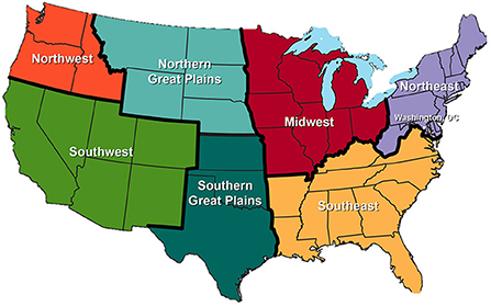
Figure 1. National Climate Assessment regions (Available online at: https://www.c2es.org/content/national-climate-assessment/). SE, southeast, NE, northeast, MW, Midwest, SGP, southern great plains, SW, southwest, NGP, northern great plains, NW, northwest.
Assessing regional changes
The quantiles' seasonal climatology of the indices (RX1, TOTs and SDII) is determined for the reference period (1951–2014). First, the indices are computed for the M (70) ensembles for N (64) years; in total, it gives M × N data points (70 ensembles of 64 years each producing 4,480 points) in each grid. Second, the quantiles (25, 50, 75, and 95th) are calculated using the data probability distribution (e.g., 25th of 4,480 values). These reference quantiles are used to normalize the future changes (trend magnitudes) of the indices and presented as percentages. The normalized changes over CONUS are cropped into the seven NCA regions (i.e., SE, NE, MW, SGP, SW, NG, and NW). The grids within an NCA region are aggregated to calculate the average change (%). The grids are also used to compute standard deviation to represent regional uncertainty in the projected changes. The normalization is applied to all the quantiles used in the study but is shown only for the 50th (median) and 95th (extreme) quantiles. The normalization produces a percent value and is used to compare the projected changes among different regions. Equation (3) explains the normalization approach.
where, Tr represents trend magnitudes (2015-2100), Climr represent reference quantiles from 1951 to 2014. r represent different quantiles, i.e., 50 and 95th, and N represents no of years during 2015–2100 period.
Results
Daily maximum
This study uses Sen's slope estimator to investigate the projected trends (2015–2100) from the distribution of ensemble members of seasonal daily maximum precipitation in various quantiles. Figure 2 illustrates the spatial distribution of the daily maximum trend magnitudes across seasons. Seasons influence the spatial patterns of the RX1, which remains consistent across quantiles with a varying range of projected trend magnitudes.
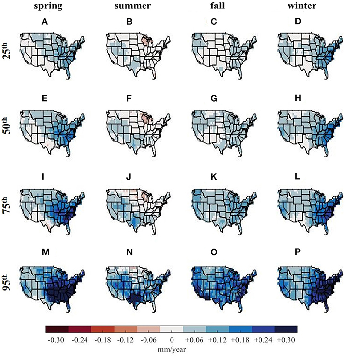
Figure 2. CONUS spatial distribution of projected daily maximum (mm) Sen's long-term trends of projected daily maximum precipitation (mm/year) from 2015 to 2100 using CESM2-LE for different quantiles (rows) across seasons (columns). Cold (blue) colors represent wetting trends, whereas warm (red) represents a drying trend, and no change is highlighted in the white color. The trend magnitudes are shown as; lower 25th [spring (A), summer (B), fall (C), and winter (D); median 50th, (E–H); above median 75th, (I–L); and extreme 95th (M–P)]. The cold (blue) color represents wetting trends, whereas warm (red) represents drying and no change is highlighted in white color. Single emission scenario SSP3-7.0 (between the moderate SSP4-6.0 and the worst-case SSP5-8.5 scenarios) is used in the analysis.
Spring shifts toward a higher wetting magnitude in the eastern regions (SE, NE), and parts of the MW, moving from the 25 to 95th quantile (Figures 2A,E,I,M). In the highest quantile, higher positive magnitudes are projected in the country's eastern half (i.e., SE, NE, and MW). The summer trends project smaller wetting patterns in lower quantiles (Figures 2B–D) in southern (SGP, SW), and northwest (NW) regions, illustrating a higher magnitude in the highest quantile except the upper MW.
Fall shows minimal to no change in the lower quantiles (Figures 2C,G) over the central U.S. but projects a positive trend in the highest quantile (95th). In winter, a positive signal in the SE, NE, and SW in the 25, 50, and 75th quantiles are found. The winter illustrates a similar spatial pattern in the eastern regions as the spring in the 95th. The seasonal and regional breakdown of trend magnitudes at different quantiles provides a complete understanding of changes in the projected distribution of the daily maximum precipitation. Most importantly, the 95th quantile (extremes) trend distribution illustrates a general wetting pattern across all seasons and regions, except for much of the NGP in summer, while the changes in the lower quantiles are much less pronounced (Figures 2M–P). There is a general wetting pattern over most regions of CONUS in the highest quantile.
Seasonal total
Spatial patterns of seasonal total (TOTs) trends are illustrated in Figure 3. A drying pattern and minimal change are found in the southern parts (SGP and SW) in spring (Figures 3A,E,I,M). In contrast wetting patterns dominate in NE, SE, and MW, stretching to the Northern Great Plains from the 50th quantile.
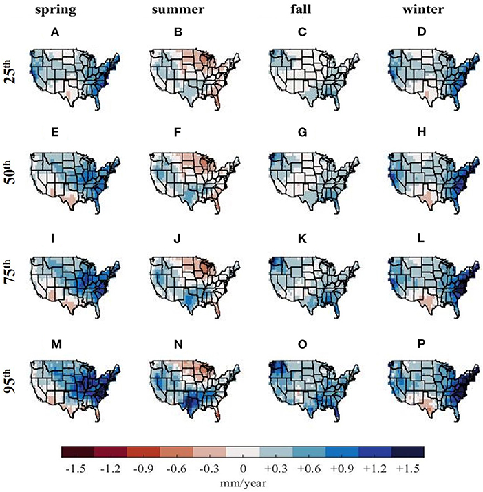
Figure 3. CONUS spatial distribution of projected seasonal total (mm/year) Sen's long-term trends of projected seasonal total (mm/year) from 2015 to 2100 using CESM2-LE for different quantiles (rows) across seasons (columns). Cold (blue) colors represent wetting trends, whereas warm (red) represents a drying trend, and no change is highlighted in the white color. The trend magnitudes are shown as; lower 25th [spring (A), summer (B), fall (C), and winter (D); median, 50th, (E–H); above median 75th, (I–L); and extreme 95th (M–P)].
The summer drying and wetting patterns are visible in MW and SGP, respectively (Figures 3B,F,J,N). The wetting pattern of fall becomes prominent in the higher quantiles with concentrated higher magnitudes in the NW, NE, and SE. No change in fall is pronounced at the lower quantiles in MW, NGP, and SW (Figures 3C,G). The winter pattern is similar to spring, except for an enhanced drying pattern in SGP, particularly in Texas. In contrast to Figure 2, TOTs trends show a mixture of regional wetting and drying patterns. These results illustrate that increases in seasonal total precipitation is most pronounced in the eastern and mid-western CONUS in spring and winter, while increases in the Gulf Coast region are focused in summer and fall. A summer drying trend is also identified across the NGP and Florida in all quantiles.
SDII
The precipitation intensity index in Figure 4 shows a consistency in the spatial pattern of spring SDII across quantiles. A general intensifying pattern is projected in SE, NE, and MW in spring precipitation intensity (Figures 4A,E,I,M). On the contrary, SW and SGP project no change to drying patterns in southern Texas. Florida is also projected to experience a drying pattern in the 95th quantile in spring.
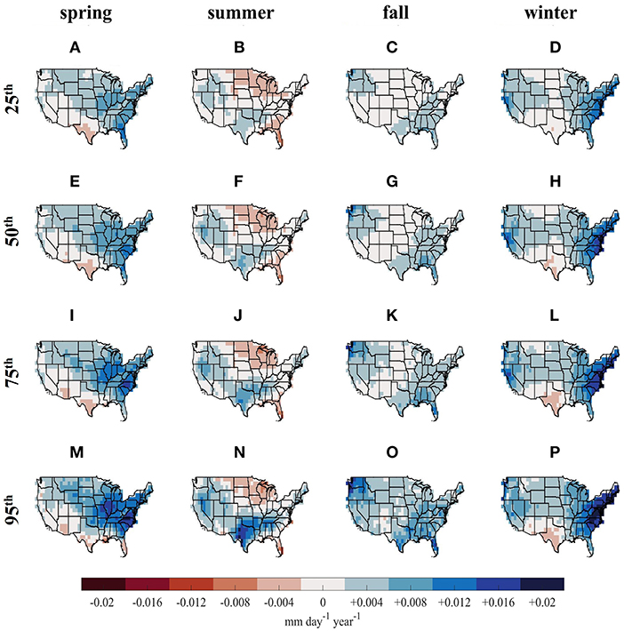
Figure 4. CONUS spatial distribution of projected SDII (mm/day/year) Sen's long-term trends of projected SDII (mm/day/year) from 2015 to 2100 using CESM2-LE for different quantiles (rows) across seasons (columns). Cold (blue) colors represent wetting trends, whereas warm (red) represents a drying trend, and no change is highlighted in the white color. The trend magnitudes are shown as; lower 25th [spring (A), summer (B), fall (C), and winter (D); median 50th, (E–H); above median 75th, (I–L); and extreme 95th (M–P)].
Summer shows a mixture of wetting and drying in addition to regions with no changes in precipitation intensity (Figures 4B,F,J,N). At the lower quantile (25th), most of NE, southern MW, and the majority of SW show no change in the daily intensity. Texas is projected to have a higher magnitude of change at the 95th quantile. Fall shows no change in NGP, MW, SW, northern SGP, and wetting patterns in the SE and NW in the 25 and 50th quantiles (Figures 4C,G). At the higher quantile, i.e., 95th many of these no-change regions are projected to have slightly intensified precipitation. Winter shows higher magnitudes of change in the NE and SE, even in the lowest quantile (25th). A similar spatial pattern is illustrated in the NGP and SGP in 25 and 50th (Figures 4D,H). At the higher quantiles, a wetting pattern is projected to cover most parts except Texas (drying).
Regional changes
Figures 5–7 illustrate normalized percent change in the NCA regions. The bars represent normalized average change (colored according to the NCA regional map, Figure 1), and error bars represent the standard deviation of the changes representing uncertainty in regional changes. Figure 5 illustrates the seasonality of such regional changes of RX1 at two quantiles, i.e., 50 and 95th. In contrast to the southern and western parts of the country, in the 50th quantile, the SE, MW, NE, and NGP exhibits larger normalized increases in spring (Figure 5A). At the 95th quantile, the standard deviation increases across regions implying the variation among the normalized pixels within a region is higher.
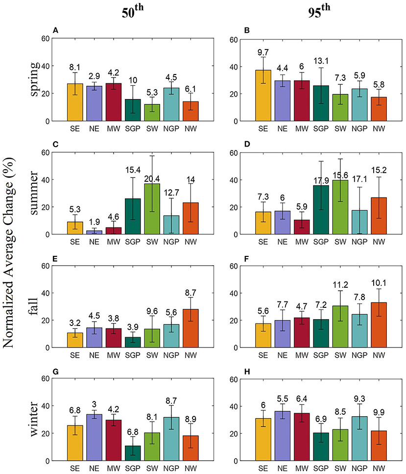
Figure 5. Normalized regional average change of maximum daily precipitation (mm) represented across seasons for the 50th and 95th quantiles compared to historical climatology from 1951 to 2014. Different color bar plots represent the regions of the National Climate Assessment (as shown in Figure 1), and the error bar represents the standard deviation of the normalized change within a region [spring (A), summer (C), fall (E), winter (G), spring (B), summer (D), fall (F), and winter (H)].
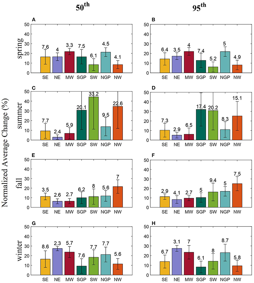
Figure 6. Normalized regional average change of maximum seasonal total (mm) represented across seasons for the 50th and 95th quantiles compared to historical climatology from 1951 to 2014. Different color bar plots represent the regions of the National Climate Assessment (as shown in Figure 1), and the error bar represents the standard deviation of the normalized change within a region [spring (A), summer (C), fall (E), winter (G), spring (B), summer (D), fall (F), and winter (H)].

Figure 7. Normalized regional average change of maximum SDII (mm/day) represented across seasons for the 50th and 95th quantiles compared to historical climatology from 1951 to 2014. Different color bar plots represent the regions of the National Climate Assessment (as shown in Figure 1), and the error bar represents the standard deviation of the normalized change within a region [spring (A), summer (C), fall (E), winter (G), spring (B), summer (D), fall (F), and winter (H)].
Summer shows a greater change in southern and western parts of CONUS (i.e., SGP, SW, NW) than in the eastern and northern parts in both the 50 and 95th quantiles (magnitude and standard deviation vary in different quantiles). Both quantiles found a higher average percent change in the NW during the fall. However, the smallest change is found in SGP at 50th and SE at 95th. The eastern (SE, NE) and northern (NGP, MW) regions have higher magnitudes of average percent change during winter. The normalized average change across regions reveals a seasonal pattern. The 95th normalized changes are bigger than the 50th in most regions.
The seasonal variation of normalized average changes in total precipitation ranges from ~+10 to +40% in Figure 6. Unlike the daily maximum, for which the Southeast shows the greatest change in the spring at 95th, the seasonal total in Midwest is shown to exhibit a greater increase (Figure 6B). Summer precipitation totals indicate bigger shifts with higher variability (standard deviation) in the southern and western regions (SW, SGP, and NW) (Figures 6C,D). On the other hand, the eastern (SE and NE) and the Midwest have the lowest shifts in both quantiles (50 and 95th). Fall (Figures 6E,F) also has a similar pattern of change as daily maximum in both quantiles (NE lowest change and NW greatest change). Except for SGP and NW, most regions see a larger change in the winter (Figures 6G,H). During the winter, however, the change in SW declined in the 95th. In general, in spring, fall, and winter, the relative rate of the total seasonal precipitation changes is similar in the middle and high-end distribution. However, higher increases are only notable in the SGP, SW, and NW during summer.
The projected changes in the intensity index are illustrated in Figure 7. MW and NGP are expected to experience greater changes on the 50 and 95th during spring (Figures 7A,B). Summer shows a higher percentage change in the southern (SGP) and western (SW and NW) regions, with 50th having a greater change than 95th (Figures 7C,D). Fall has a relatively smaller change in each region compared to other seasons (Figures 7E,F). The pattern of change in each region is similar for both the quantiles during fall. The NE region is projected to have the greatest change among the rest regions during winter (both 50 and 95th), followed by MW (Figures 7G,H). The intensity index also has a seasonal dependency on the average change across the region. Even though the average shift varies by region, a similar regional shift is expected in the seasonal total.
Trend detection is studied in each ensemble distribution of the RX1, TOTs and SDII to explore the uncertainty in detecting a trend from the ensemble distribution. We define a grid as capturing the sign of change if it detects a statistically significant trend and the majority (>50%) of the ensembles agree on that detection. The RX1 trend varies with season, resulting in varying ensemble agreements. For example, fall agrees on no trend in the eastern areas, winter agrees on a positive trend in the eastern regions, summer agrees on no trend in the western regions, and spring agrees on no trend in most regions (except MW and SE) in Table 1.
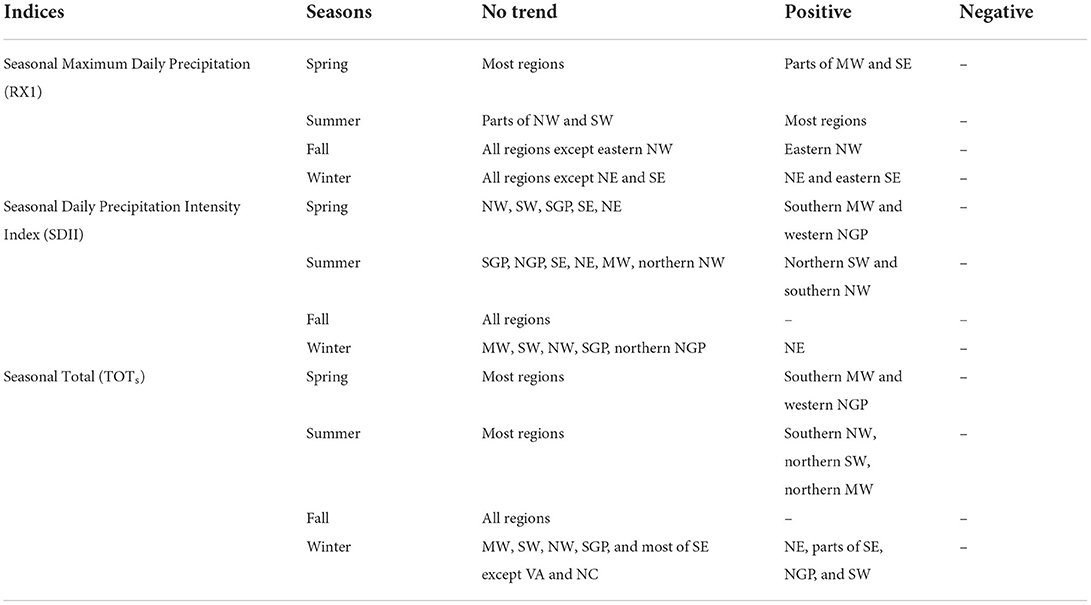
Table 1. Ensemble agreement on the signs of change (no trend, 0; positive trend, +1; and negative trend, −1) across the indices, i.e., RX1 (mm), TOTs (mm), and SDII (mm/day) in each season.
SDII shows a different trend detection than RX1 in summer, where parts of the southwest agree on positive trends. However, the regional agreement shows similar results in winter (NE positive) and fall (no trends in most regions). An increasing trend in the eastern (NE, SE) and northern plains is detected in winter. The eastern regions agree on positive trends in the three indices.
Discussion
Understanding the Earth's hydroclimatic response to global warming necessitates knowledge of changes in mean precipitation and other distributions (Giorgi et al., 2019). The study demonstrates projected long-term (2015–2100, under SSP3-7.0) trends of extreme daily maximum and precipitation intensity indices (RX1 and SDII) and precipitation climatology (TOTs) at regional and seasonal scales over CONUS using CESM2-LE simulations. The long-term trend of these indices is characterized across a range of quantiles. Since LEs can circumvent the issue of complex model uncertainties created by averaging different climate models (Deser et al., 2012), the ensemble mean allows for studying externally imposed changes in precipitation as the mean reduces the internal variability (Zhang and Delworth, 2018).
In general, we find that the spatial distribution of extreme indices at different quantiles projects a wetter extreme over most of the regions of CONUS toward the end of the twenty-first century in SSP3-7.0. The indices exhibit regional patterns with wetting in the northeastern regions during spring and winter and relative drying in the MW in summer. Figure 2 illustrates that most SE region shows projected wetting in daily maximum summer at the 95th quantile. TOTs (Figure 3) and SDII (Figure 4) show similar spatial patterns as Figure 2 at the 95th quantile, and the wetting is mostly concentrated over the southern part of the domain. The TOTs in Figure 3 show a drying summer in NGP and a wetting winter in NE and SE. Our findings complement a study by Hayhoe et al. (2007) that illustrates a consistent increase in winter but no change to the drying during summer in the NE in nine atmosphere-ocean general circulation model simulations (AOGCMs). Marvel et al. (2021) corroborate the increasing amplitude of NW and SE during the winter-wet season. Akinsanola et al. (2020b) employed CMIP6 models to investigate variations in extreme summer and winter precipitation over the U.S., finding that winter precipitation intensity is expected to increase in the twenty-first century. While the authors illustrate model agreement on the winter increase, models agree less during summer.
Our results show that the MW will experience wetting in spring by the end of the twenty-first century under the mid to high emission scenario. The finding is consistent with a recent study by Grady et al. (2021), which finds a regional increase in projected wet spring in the late-century (30-year study period) in the downscaled CMIP5 RCP8.5. Feng et al. (2016) explain the changing characteristics of spring mesoscale convective systems (MCSs) that dominate the central US and the increased rainfall that results. Pressure gradient increases caused by surface warming over Rocky Mountain were identified as a potential cause of the MCSs changing characteristics in the earlier study, spanning from 1979 to 2014. A wetting pattern also dominates in the Midwest regions during spring at the 95th quantile (Figure 3). Cook et al. (2008) found that warming temperatures intensify the low-level jet, resulting in more spring precipitation in the upper MW. High-resolution modeling efforts with convection-permitting models (CPMs) will be beneficial for understanding the mechanisms of MCSs and the associated changes in spring total precipitation.
The projected changes in Figures 2, 3 show that the MW and eastern regions (NE, SE) are expected to have greater changes in RX1 and SDII during spring and winter. In contrast, summer is expected to change the most in the southern parts of the country (SW, SGP). In the NW, a noticeable change is expected in the fall. The SW region varies from no change to drying in TOTs and SDII during spring. In a warmer climate, the Southwest's water availability is projected to decline during spring (due to decreased precipitation and increased evapotranspiration) (Gao et al., 2014). Figure 2 shows that the southeast is projected to have a higher magnitude increase in the 95th quantile of RX1. A previous study attributes the intense precipitation in the SE fall to tropical cyclones (Dourte et al., 2015). Summer daily maximum trend magnitudes at lower quantiles (25, 50, 75th) project no change in the upper MW, which is in the drying range in the seasonal total precipitation trends.
In conclusion, the three research questions set in the Introduction are addressed as follows:
1. How is future precipitation expected to vary in extreme indices across quantiles seasonally in the twenty-first century? Our results corroborate findings from previous studies on the projected change of extreme indices, showing that the magnitude of change depends on seasons, regions, and the index itself. Extreme indices (getting either drier or wetter) also vary among quantiles, making it difficult to provide a single answer to this question. For instance, fall precipitation accumulations in the central US show trend magnitudes ranging from no change in the lower quantiles (i.e., 25, 50th) to wetting trends in the highest quantile (95th).
2. Which quantiles are more likely to drive future precipitation changes? As stated above, the spatial patterns of trends depend on seasonality. With a few exceptions, the three indices used in the study show similar spatial patterns of trend magnitudes, implying that seasonal climatology, daily maximum, and daily intensity are projected to have similar spatial patterns. In particular, the highest quantile analyzed in the study, i.e., 95th, is most likely to drive higher wetting trends, especially in the NE and the SE US in spring and winter.
3. What changes in precipitation are likely to occur at the regional scale, and what are the associated uncertainties? Normalized average changes (representing regional changes) show consistent seasonal patterns among the three indices. Positive and statistically significant trends are found in the eastern parts of the country during winter and in the MW during spring. No regions with dominant negative trends were identified in this study.
Lastly, this study attempts to provide a robust estimation of the seasonal change in extreme indices and climatology across different regions of CONUS. The study uses an ensemble of simulations to increase the sample size and evaluate the changes of future extreme quantiles (end of the twenty-first century) to that of the climatological quantiles of the earlier century in a new “scenario-matrix architecture” (SSP3-7.0). Outcomes from this work advance our understanding of extreme precipitation in the latest large ensemble spread of the Community Earth System Model.
Conclusion
This study analyzes the large ensemble of the CESM-2 for a medium to high emission scenario range (SSP3-7.0) in terms of daily maximum in a seasonal window, seasonal total, and daily precipitation intensity. We compare the projected changes of selected quantiles to the climatology of those quantiles (1951–2014). Examining the future extreme precipitation change of distinct quantiles provides insights into the variability of regional precipitation regimes.
Projected seasonal climatology (TOTs) shows wetting and drying patterns, specifically wetter spring and winter in the eastern regions with drying summer in the Midwest. We have seen uncertainties within ensembles in detecting trends, further influenced by seasons and indices. Among all the indices employed in the study, the northern regions, particularly the NE and SE, consistently detect increasing projected trends during winter. In the fall, most regions exhibit no trend in any indices considered. The central U.S. is projected to have no change at lower quantiles which transitions to wetting at the 95th quantile in fall. On the other hand, the seasonal daily maximum is projected to have an overall wetting pattern at the 95th quantile. Results also show that the normalized average change in fall is minimal across the indices and consistent across different parts of the distribution (50 and 95th). The spatial distribution of projected trends primarily represents the climatological patterns in different parts of CONUS. Because climate models' coarse resolution limits their ability to accurately depict precipitation at the local scale, the magnitudes of the trends may not be well simulated at the local to subregional scale. Numerous studies discussed the systematic biases of the global and regional climate models in simulating the precipitation properties, which result in overly-frequent light precipitation and an underestimation of extreme precipitation (Kharin et al., 2005). When convection-permitting models (CPMs) become available for climate simulation, the identified patterns at the regional scale may be better captured in terms of magnitudes. Additionally, to better understand wetting and drying patterns, future studies should concentrate on long-term trends in other hydrological variables, such as evaporation and soil moisture, along with extreme precipitation changes. Incorporating other wet and dry extreme indices and other emission scenarios will aid in the development of comprehensive regional analyses of precipitation.
Despite the model uncertainties, investigating the projected changes in upper and lower quantiles of extreme indices can provide insight into regional vulnerability to wet and dry extremes in a warmer climate by considering many simulations. Also, while examining the trends captured within the models may not necessarily predict the exact magnitudes of precipitation changes, it can provide a valuable tool in determining the relative rate of precipitation changes across CONUS. Exploring the regional response in projected precipitation in emission scenario SSP3-7.0 from only a single large ensemble (CESM2-LE) is one of the limitations of the present study. However, the inclusion of multi-model simulations in the current approach should provide a robust signal in exploring the changing characteristics of climatology and extreme indices. Moreover, future research incorporating such analysis under different emission scenarios is expected to provide insight into the full range of uncertainties emerging from differences in modeling structure and methods applied. Furthermore, regional climate models are likely to provide geographical variability in the projected trends, but they are computationally expensive; therefore, LE simulations are useful for exploring projected regional changes in extremes and the associated uncertainties.
Data availability statement
The National Center for Atmospheric Research (NCAR) has made the CESM2 Large Ensemble simulations publicly available at http://www.cesm.ucar.edu/CESM2-LENS2/.
Author contributions
ID investigated extreme precipitation trends, created figures and table, collated the main takeaways, prepared the original manuscript, and reviewed it. VM provided reviews, led project scoping, and guided in connecting finding to the project scoping. JJ contributed to project scoping, performed draft revision, and assisted in connecting findings to the project scoping. GC supported the team with downloading and cropping the CESM2-LE (100 km/daily) dataset to CONUS grid boxes and leading project scoping. JK performed draft revision and provided feedbacks on the project scoping and findings. All authors contributed to the reviewing and editing of the original manuscript.
Acknowledgments
The authors acknowledge the CESM2 Large Ensemble Community Project for providing data. The datasets are analyzed on the HOPPER Cluster, which is managed by George Mason University's Office of Research Computing (orc.gmu.edu).
Conflict of interest
The authors declare that the research was conducted in the absence of any commercial or financial relationships that could be construed as a potential conflict of interest.
Publisher's note
All claims expressed in this article are solely those of the authors and do not necessarily represent those of their affiliated organizations, or those of the publisher, the editors and the reviewers. Any product that may be evaluated in this article, or claim that may be made by its manufacturer, is not guaranteed or endorsed by the publisher.
References
Abdelmoaty, H. M., Papalexiou, S. M., Rajulapati, C. R., and AghaKouchak, A. (2021). Biases beyond the mean in CMIP6 extreme precipitation: a global investigation. Earth's Future 9:e2021EF002196. doi: 10.1029/2021EF002196
Akinsanola, A. A., Kooperman, G. J., Pendergrass, A. G., Hannah, W. M., and Reed, K. A. (2020a). Seasonal representation of extreme precipitation indices over the United States in CMIP6 present-day simulations. Environ. Res. Lett. 15:094003. doi: 10.1088/1748-9326/ab92c1
Akinsanola, A. A., Kooperman, G. J., Reed, K. A., Pendergrass, A. G., and Hannah, W. M. (2020b). Projected changes in seasonal precipitation extremes over the United States in CMIP6 simulations. Environ. Res. Lett. 15:104078. doi: 10.1088/1748-9326/abb397
Akinsanola, A. A., Ongoma, V., and Kooperman, G. J. (2021). Evaluation of CMIP6 models in simulating the statistics of extreme precipitation over Eastern Africa. Atmos. Res. 254:105509. doi: 10.1016/j.atmosres.2021.105509
Alexander, L. V., Zhang, X., Peterson, T. C., Caesar, J., Gleason, B., Klein Tank, A. M. G., et al. (2006). Global observed changes in daily climate extremes of temperature and precipitation. J. Geophys. Res. 111:D05109. doi: 10.1029/2005JD006290
Allan, R. P., and Soden, B. J. (2008). Atmospheric warming and the amplification of precipitation extremes. Science 321, 1481–1484. doi: 10.1126/science.1160787
Allen, M. R., and Ingram, W. J. (2002). Constraints on future changes in climate and the hydrologic cycle. Nature 419, 228–232. doi: 10.1038/nature01092
Anderson, T. R., Hawkins, E., and Jones, P. D. (2016). CO2, the greenhouse effect and global warming: from the pioneering work of Arrhenius and Callendar to today's Earth system models. Endeavour 40, 178–187. doi: 10.1016/j.endeavour.2016.07.002
Ayugi, B., Dike, V., Ngoma, H., Babaousmail, H., Mumo, R., and Ongoma, V. (2021). Future changes in precipitation extremes over East Africa based on CMIP6 models. Water 13:2358. doi: 10.3390/w13172358
Bartolini, G., Grifoni, D., Torrigiani, T., Vallorani, R., Meneguzzo, F., and Gozzini, B. (2014). Precipitation changes from two long-term hourly datasets in Tuscany, Italy. Int. J. Climatol. 34, 3977–3985. doi: 10.1002/joc.3956
Benestad, R. E. (2018). Implications of a decrease in the precipitation area for the past and the future. Environ. Res. Lett. 13:044022. doi: 10.1088/1748-9326/aab375
Coelho, G. D. A., Ferreira, C. M., Johnston, J., Kinter, J. L., Dollan, I. J., et al. (2022). Potential Impacts of future extreme precipitation changes on flood engineering design across the Contiguous United States. Water Resour. Res. 58:e2021WR031432. doi: 10.1029/2021WR031432
Cook, B. I., Ault, T. R., and Smerdon, J. E. (2015). Unprecedented twenty-first century drought risk in the American Southwest and Central Plains. Sci. Adv. 1:e1400082. doi: 10.1126/sciadv.1400082
Cook, K. H., Vizy, E. K., Launer, Z. S., and Patricola, C. M. (2008). Springtime intensification of the great plains low-level jet and midwest precipitation in GCM simulations of the twenty-first century. J. Clim. 21, 6321–6340. doi: 10.1175/2008JCLI2355.1
Dai, A. (2013). Increasing drought under global warming in observations and models. Nat. Clim. Change 3, 52–58. doi: 10.1038/nclimate1633
Danabasoglu, G., Lamarque, J. -F., Bacmeister, J., Bailey, D. A., DuVivier, A. K., Edwards, J., et al. (2020). The Community Earth System Model Version 2 (CESM2). J. Adv. Model. Earth Syst. 12:e2019MS001916. doi: 10.1029/2019MS001916
Deser, C., Phillips, A., Bourdette, V., and Teng, H. (2012). Uncertainty in climate change projections: the role of internal variability. Clim. Dyn. 38, 527–546. doi: 10.1007/s00382-010-0977-x
Diaconescu, E. P., Gachon, P., Laprise, R., and Scinocca, J. F. (2016). Evaluation of precipitation indices over North America from various configurations of regional climate models. Atmosphere-Ocean 54, 418–439. doi: 10.1080/07055900.2016.1185005
Dollan, I. J., Maggioni, V., and Johnston, J. (2022). Investigating temporal and spatial precipitation patterns in the Southern Mid-Atlantic United States. Front. Clim. 3:799055. doi: 10.3389/fclim.2021.799055
Donat, M. G., Alexander, L. V., Yang, H., Durre, I., Vose, R., Dunn, R. J. H., et al. (2013). Updated analyses of temperature and precipitation extreme indices since the beginning of the twentieth century: The HadEX2 dataset: HADEX2-Global Gridded Climate extremes. J. Geophys. Res. Atmos. 118, 2098–2118. doi: 10.1002/jgrd.50150
Dong, T., and Dong, W. (2021). Evaluation of extreme precipitation over Asia in CMIP6 models. Clim. Dyn. 57, 1751–1769. doi: 10.1007/s00382-021-05773-1
Dourte, D. R., Fraisse, C. W., and Bartels, W.-L. (2015). Exploring changes in rainfall intensity and seasonal variability in the Southeastern U.S.: stakeholder engagement, observations, and adaptation. Clim. Risk Manage. 7, 11–19. doi: 10.1016/j.crm.2015.02.001
Douville, H., Raghavan, K., Renwick, J., Allan, R. P., Arias, P. A., Barlow, M., et al. (2021). “Water cycle changes,” in Climate Change 2021: The Physical Science Basis. Contribution of Working Group I to the Sixth Assessment Report of the Intergovernmental Panel on Climate Change, eds V. Masson-Delmotte, P. Zhai, A. Pirani, S. L. Connors, C. Péan, S. Berger, N. Caud, Y. Chen, L. Goldfarb, M.I. Gomis, M. Huang, K. Leitzell, E. Lonnoy, J. B. R. Matthews, T. K. Maycock, T. Waterfield, O. Yelek?i, R. Yu, and B. Zhou (Cambridge; New York, NY: Cambridge University Press), 1055–1210. doi: 10.1017/9781009157896.010
Eyring, V., Bony, S., Meehl, G. A., Senior, C. A., Stevens, B., Stouffer, R. J., et al. (2016). Overview of the coupled model intercomparison project phase 6 (CMIP6) experimental design and organization. Geosci. Model Dev. 9, 1937–1958. doi: 10.5194/gmd-9-1937-2016
Feng, Z., Leung, L. R., Hagos, S., Houze, R. A., Burleyson, C. D., and Balaguru, K. (2016). More frequent intense and long-lived storms dominate the springtime trend in central US rainfall. Nat. Commun. 7:13429. doi: 10.1038/ncomms13429
Fischer, E. M., Beyerle, U., and Knutti, R. (2013). Robust spatially aggregated projections of climate extremes. Nat. Clim. Change 3, 1033–1038. doi: 10.1038/nclimate2051
Fischer, E. M., and Knutti, R. (2016). Observed heavy precipitation increase confirms theory and early models. Nat. Clim. Change 6, 986–991. doi: 10.1038/nclimate3110
Gao, Y., Leung, L. R., Lu, J., Liu, Y., Huang, M., and Qian, Y. (2014). Robust spring drying in the southwestern U.S. and seasonal migration of wet/dry patterns in a warmer climate: future water availability changes. Geophys. Res. Lett. 41, 1745–1751. doi: 10.1002/2014GL059562
Giorgi, F., Coppola, E., and Raffaele, F. (2014). A consistent picture of the hydroclimatic response to global warming from multiple indices: models and observations: hydroclimatic response to global warming. J. Geophys. Res. Atmos. 119, 11,695–11,708. doi: 10.1002/2014JD022238
Giorgi, F., Raffaele, F., and Coppola, E. (2019). The response of precipitation characteristics to global warming from climate projections. Earth Syst. Dyn. 10, 73–89. doi: 10.5194/esd-10-73-2019
Gleckler, P. J., Taylor, K. E., and Doutriaux, C. (2008). Performance metrics for climate models. J. Geophys. Res. 113:D06104. doi: 10.1029/2007JD008972
Grady, K. A., Chen, L., and Ford, T. W. (2021). Projected changes to spring and summer precipitation in the Midwestern United States. Front. Water 3:780333. doi: 10.3389/frwa.2021.780333
Hayhoe, K., Wake, C. P., Huntington, T. G., Luo, L., Schwartz, M. D., Sheffield, J., et al. (2007). Past and future changes in climate and hydrological indicators in the US Northeast. Clim. Dyn. 28, 381–407. doi: 10.1007/s00382-006-0187-8
Held, I. M., and Soden, B. J. (2006). Robust responses of the hydrological cycle to global warming. J. Clim. 19, 5686–5699. doi: 10.1175/JCLI3990.1
IPCC (2014). “Climate change 2014: Synthesis report,” in Contribution of Working Groups I, II and III to the Fifth Assessment Report of the Intergovernmental Panel on Climate Change, eds Core Writing Team, R. K. Pachauri, and L. A. Meyer (Geneva: IPCC), 151.
IPCC (2021). Climate Change 2021: The Physical Science Basis. Available online at: https://www.ipcc.ch/report/ar6/wg1/
John, A., Douville, H., Ribes, A., and Yiou, P. (2022). Quantifying CMIP6 model uncertainties in extreme precipitation projections. Weather Clim. Extrem. 36:100435. doi: 10.1016/j.wace.2022.100435
Kharin, V. V., Zwiers, F. W., and Zhang, X. (2005). Intercomparison of near-surface temperature and precipitation extremes in AMIP-2 simulations, reanalyses, and observations. J. Clim. 18, 5201–5223. doi: 10.1175/JCLI3597.1
Kumar, S., Merwade, V., Kinter, J. L., and Niyogi, D. (2013). Evaluation of temperature and precipitation trends and long-term persistence in CMIP5 twentieth-century climate simulations. J. Clim. 26, 4168–4185. doi: 10.1175/JCLI-D-12-00259.1
Lausier, A. M., and Jain, S. (2018). Overlooked trends in observed global annual precipitation reveal underestimated risks. Sci. Rep. 8:16746. doi: 10.1038/s41598-018-34993-5
Li, C., Zwiers, F., Zhang, X., Li, G., Sun, Y., and Wehner, M. (2021a). Changes in annual extremes of daily temperature and precipitation in CMIP6 models. J. Clim. 34, 3441–3460. doi: 10.1175/JCLI-D-19-1013.1
Li, J., Huo, R., Chen, H., Zhao, Y., and Zhao, T. (2021b). Comparative assessment and future prediction using CMIP6 and CMIP5 for annual precipitation and extreme precipitation simulation. Front. Earth Sci. 9:687976. doi: 10.3389/feart.2021.687976
Madsen, H., Lawrence, D., Lang, M., Martinkova, M., and Kjeldsen, T. R. (2014). Review of trend analysis and climate change projections of extreme precipitation and floods in Europe. J. Hydrol. 519, 3634–3650. doi: 10.1016/j.jhydrol.2014.11.003
Mann, H. B. (1945). Nonparametric tests against trend. Econometrica 13, 245–259. doi: 10.2307/1907187
Marvel, K., Cook, B. I., Bonfils, C., Smerdon, J. E., Williams, A. P., and Liu, H. (2021). Projected changes to hydroclimate seasonality in the Continental United States. Earth's Future 9:e2021EF002019. doi: 10.1029/2021EF002019
Melillo, J. M., Richmond, T. C., and Yohe, G. W. (2014). Climate Change Impacts in the United States: The Third National Climate Assessment. U.S. Global Change Research Program. doi: 10.7930/J0Z31WJ2
Ménégoz, M., Valla, E., Jourdain, N. C., Blanchet, J., Beaumet, J., Wilhelm, B., et al. (2020). Contrasting seasonal changes in total and intense precipitation in the European Alps from 1903 to 2010. Hydrol. Earth Syst. Sci. 24, 5355–5377. doi: 10.5194/hess-24-5355-2020
O'Gorman, P. A., and Muller, C. J. (2010). How closely do changes in surface and column water vapor follow Clausius–Clapeyron scaling in climate change simulations? Environ. Res. Lett. 5:025207. doi: 10.1088/1748-9326/5/2/025207
Papalexiou, S. M., and Montanari, A. (2019). Global and regional increase of precipitation extremes under global warming. Water Resour. Res. 55, 4901–4914. doi: 10.1029/2018WR024067
Pendergrass, A. G., and Hartmann, D. L. (2014). Changes in the distribution of rain frequency and intensity in response to global warming*. J. Clim. 27, 8372–8383. doi: 10.1175/JCLI-D-14-00183.1
Peters-Lidard, C. D., Rose, K. C., Kiang, J. E., Strobel, M. L., Anderson, M. L., Byrd, A. R., et al. (2021). Indicators of climate change impacts on the water cycle and water management. Clim. Change 165:36. doi: 10.1007/s10584-021-03057-5
Pfahl, S., O'Gorman, P. A., and Fischer, E. M. (2017). Understanding the regional pattern of projected future changes in extreme precipitation. Nat. Clim. Change 7, 423–427. doi: 10.1038/nclimate3287
Prein, A. F., Rasmussen, R. M., Ikeda, K., Liu, C., Clark, M. P., and Holland, G. J. (2017). The future intensification of hourly precipitation extremes. Nat. Clim. Change 7, 48–52. doi: 10.1038/nclimate3168
Rahat, S. H., Steinschneider, S., Kucharski, J., Arnold, W., Olzewski, J., Walker, W., et al. (2022). Characterizing hydrologic vulnerability under nonstationary climate and antecedent conditions using a process-informed stochastic weather generator. J. Water Resour. Plann. Manage. 148. doi: 10.1061/(ASCE)WR.1943-5452.0001557
Rajczak, J., and Schär, C. (2017). Projections of future precipitation extremes over Europe: a multimodel assessment of climate simulations: projections of precipitation extremes. J. Geophys. Res. Atmos. 122, 10,773–10,800. doi: 10.1002/2017JD027176
Razavi, T., Switzman, H., Arain, A., and Coulibaly, P. (2016). Regional climate change trends and uncertainty analysis using extreme indices: a case study of Hamilton, Canada. Clim. Risk Manage. 13, 43–63. doi: 10.1016/j.crm.2016.06.002
Reidmiller, D. R., Avery, C. W., Easterling, D. R., Kunkel, K. E., Lewis, K. L. M., Maycock, T. K., et al. (2018). Impacts, Risks, and Adaptation in the United States: Fourth National Climate Assessment, Vol. II. U.S. Global Change Research Program, 186. doi: 10.7930/NCA4.2018
Riahi, K., van Vuuren, D. P., Kriegler, E., Edmonds, J., O'Neill, B. C., Fujimori, S., et al. (2017). The shared socioeconomic pathways and their energy, land use, and greenhouse gas emissions implications: an overview. Glob. Environ. Change 42, 153–168. doi: 10.1016/j.gloenvcha.2016.05.009
Rodgers, K. B., Lee, S.-S., Rosenbloom, N., Timmermann, A., Danabasoglu, G., Deser, C., et al. (2021a). Ubiquity of human-induced changes in climate variability. Earth Syst. Dyn. 12, 1393–1411. doi: 10.5194/esd-12-1393-2021
Rodgers, K. B., Lee, S.-S., Rosenbloom, N., Timmermann, A., Danabasoglu, G., Deser, C., et al. (2021b). Ubiquity of human-induced changes in climate variability [Preprint]. Earth Syst. Change Clim. Scenarios. 12, 1393–411. doi: 10.5194/esd-2021-50
Schwalm, C. R., Anderegg, W. R. L., Michalak, A. M., Fisher, J. B., Biondi, F., Koch, G., et al. (2017). Global patterns of drought recovery. Nature 548, 202–205. doi: 10.1038/nature23021
Sen, P. K. (1968). Estimates of the regression coefficient based on Kendall's Tau. J. Am. Stat. Assoc. 63, 1379–1389. doi: 10.1080/01621459.1968.10480934
Sillmann, J., Kharin, V. V., Zhang, X., Zwiers, F. W., and Bronaugh, D. (2013). Climate extremes indices in the CMIP5 multimodel ensemble: part 1. Model evaluation in the present climate. J. Geophys. Res. Atmos. 118, 1716–1733. doi: 10.1002/jgrd.50203
Solomon, S., Qin, D., Manning, M., Chen, Z., Marquis, M., Averyt, K., et al. (2007). Climate Change 2007: The Physical Science Basis. Cambridge, UK; New York, NY, USA: Cambridge University Press, p. 996.
Srivastava, A., Grotjahn, R., and Ullrich, P. A. (2020). Evaluation of historical CMIP6 model simulations of extreme precipitation over contiguous US regions. Weather Clim. Extrem. 29:100268. doi: 10.1016/j.wace.2020.100268
Stouffer, R. J., Eyring, V., Meehl, G. A., Bony, S., Senior, C., Stevens, B., et al. (2017). CMIP5 scientific gaps and recommendations for CMIP6. Bull. Am. Meteorol. Soc. 98, 95–105. doi: 10.1175/BAMS-D-15-00013.1
Tabari, H. (2020). Climate change impact on flood and extreme precipitation increases with water availability. Sci. Rep. 10:13768. doi: 10.1038/s41598-020-70816-2
Taylor, K. E., Stouffer, R. J., and Meehl, G. A. (2012). An overview of CMIP5 and the experiment design. Bull. Am. Meteorol. Soc. 93, 485–498. doi: 10.1175/BAMS-D-11-00094.1
Tebaldi, C., Debeire, K., Eyring, V., Fischer, E., Fyfe, J., Friedlingstein, P., et al. (2021). Climate model projections from the Scenario Model Intercomparison project (ScenarioMIP) of CMIP6. Earth Syst. Dyn. 12, 253–293. doi: 10.5194/esd-12-253-2021
Thackeray, C. W., DeAngelis, A. M., Hall, A., Swain, D. L., and Qu, X. (2018). On the connection between global hydrologic sensitivity and regional wet extremes. Geophys. Res. Lett. 45, 11,343–11,351. doi: 10.1029/2018GL079698
Theil, H. (1950). A rank-invariant method of linear and polynomial regression analysis, 1-2; confidence regions for the parameters of linear regression equations in two, three and more variables. Stichting Mathematisch Centrum, 1950-01–01. Available online at: https://ir.cwi.nl/pub/18445
Trenberth, K. E. (1999). Conceptual framework for changes of extremes of the hydrological cycle with climate change. Clim. Change 42, 327–339. doi: 10.1023/A:1005488920935
Trenberth, K. E., Dai, A., Rasmussen, R. M., and Parsons, D. B. (2003). The changing character of precipitation. Bull. Am. Meteorol. Soc. 84, 1205–1218. doi: 10.1175/BAMS-84-9-1205
Treppiedi, D., Cipolla, G., Francipane, A., and Noto, L. V. (2021). Detecting precipitation trend using a multiscale approach based on quantile regression over a Mediterranean area. Int. J. Climatol. 41, 5938–5955. doi: 10.1002/joc.7161
van Vuuren, D. P., Edmonds, J., Kainuma, M., Riahi, K., Thomson, A., Hibbard, K., et al. (2011). The representative concentration pathways: An overview. Clim. Change 109, 5–31. doi: 10.1007/s10584-011-0148-z
van Vuuren, D. P., Kriegler, E., O'Neill, B. C., Ebi, K. L., Riahi, K., Carter, T. R., et al. (2014). A new scenario framework for climate change research: scenario matrix architecture. Clim. Change 122, 373–386. doi: 10.1007/s10584-013-0906-1
Vicente-Serrano, S. M., García-Herrera, R., Peña-Angulo, D., Tomas-Burguera, M., Domínguez-Castro, F., Noguera, I., et al. (2022). Do CMIP models capture long-term observed annual precipitation trends? Clim. Dyn. 58, 2825–2842. doi: 10.1007/s00382-021-06034-x
Villarini, G., Smith, J. A., Baeck, M. L., Vitolo, R., Stephenson, D. B., and Krajewski, W. F. (2011). On the frequency of heavy rainfall for the Midwest of the United States. J. Hydrol. 400, 103–120. doi: 10.1016/j.jhydrol.2011.01.027
Westra, S., Alexander, L. V., and Zwiers, F. W. (2013). Global increasing trends in annual maximum daily precipitation. J. Clim. 26, 3904–3918. doi: 10.1175/JCLI-D-12-00502.1
Westra, S., Fowler, H. J., Evans, J. P., Alexander, L. V., Berg, P., Johnson, F., et al. (2014). Future changes to the intensity and frequency of short-duration extreme rainfall: future intensity of sub-daily rainfall. Rev. Geophys. 52, 522–555. doi: 10.1002/2014RG000464
Zhang, H., and Delworth, T. L. (2018). Robustness of anthropogenically forced decadal precipitation changes projected for the twenty-first century. Nat. Commun. 9:1150. doi: 10.1038/s41467-018-03611-3
Keywords: long-term trend, extremes, large ensemble, CONUS, SSP3-7.0
Citation: Dollan IJ, Maggioni V, Johnston J, Coelho GdA and Kinter JL III (2022) Seasonal variability of future extreme precipitation and associated trends across the Contiguous U.S. Front. Clim. 4:954892. doi: 10.3389/fclim.2022.954892
Received: 27 May 2022; Accepted: 28 September 2022;
Published: 20 October 2022.
Edited by:
Chris C. Funk, University of California, Santa Barbara, United StatesReviewed by:
Xiaomeng Song, China University of Mining and Technology, ChinaManuchehr Farajzadeh, Tarbiat Modares University, Iran
Copyright © 2022 Dollan, Maggioni, Johnston, Coelho and Kinter. This is an open-access article distributed under the terms of the Creative Commons Attribution License (CC BY). The use, distribution or reproduction in other forums is permitted, provided the original author(s) and the copyright owner(s) are credited and that the original publication in this journal is cited, in accordance with accepted academic practice. No use, distribution or reproduction is permitted which does not comply with these terms.
*Correspondence: Ishrat Jahan Dollan, aWRvbGxhbkBnbXUuZWR1