
94% of researchers rate our articles as excellent or good
Learn more about the work of our research integrity team to safeguard the quality of each article we publish.
Find out more
ORIGINAL RESEARCH article
Front. Clim., 02 June 2022
Sec. Predictions and Projections
Volume 4 - 2022 | https://doi.org/10.3389/fclim.2022.897498
This article is part of the Research TopicMulti-Scale Air-Sea Variability and its Application in Indo-Pacific RegionsView all 8 articles
 Yoshi N. Sasaki1*
 Yuma Iwai2
Subduction and migration of density-compensated (warm/salty or cool/fresh) temperature and salinity water-mass anomalies on isopycnals, referred to as spiciness anomalies, are examined in the subtropical gyre of the South Pacific using an observational dataset. The present results demonstrate that the spiciness anomalies are found to follow two pathways from the subtropical region to the tropical area on the 25–25.5σθ isopycnals. The water masses of one pathway subduct south of 20°S and mainly flow westward via the mean geostrophic current to the western boundary region. The water masses of this pathway correspond to the salinity maximum on these isopycnals as well as the bottom of the South Pacific Tropical Water. Positive temperature and salinity trends were prominent along this pathway during the study period. In the other pathway, the water masses subduct north of 20°S and go directly to the tropics through the interior region. Decadal variability of the spiciness anomalies is prominent along this pathway. In both pathways, sea surface salinity variability likely plays an important role in generating the spiciness anomalies on the isopycnals. A passive tracer experiment revealed that the advection by the South Equatorial Countercurrent (SECC) divides these two pathways. Hence, SECC plays a key role in determining whether a spiciness anomaly propagates through the interior region or the western boundary region.
Subduction is an important aspect of ocean circulation (e.g., Qiu and Huang, 1995). The water mass subducted at the sea surface carries its properties such as heat, salt, and oxygen into the subsurface ocean. The subduction process transports water mass properties not only vertically but also horizontally. Previous studies suggested that the subduction process is related to decadal variability in the subtropics and tropics. Many studies reported based on numerical simulation that variability in the subtropics can influence variability in the tropics through the subsurface pathway (e.g., Nonaka and Xie, 2000; Pierce et al., 2000; Fukumori et al., 2004; Ogata and Nonaka, 2020). There are two mechanisms of signal propagation from the subtropics to the tropics associated with the subduction. One is higher modes of Rossby waves (e.g., Liu, 1999), and the other is the propagation of density-compensated temperature and salinity anomalies (hereafter referred spiciness anomaly) on isopycnals. Several numerical studies showed the importance of the latter mechanism (e.g., Gu and Philander, 1997; Yeager and Large, 2004; Taguchi and Schneider, 2014), but observational studies were limited. This was because the former signals (i.e., higher modes of Rossby waves) can be seen only from temperature observations (e.g., Schneider et al., 1999), but not only temperature but also salinity observations were needed to investigate the signals associated with the latter mechanism.
The advent of the Argo observations made it possible to examine basin-wide propagation of spiciness anomalies. Sasaki et al. (2010) presented the first evidence of the observed spiciness anomaly propagation in the North Pacific based on Argo data from 2003 to 2008. Similar propagation signals have been reported in other depths and other ocean basins (e.g., Kolodziejczyk and Gaillard, 2012; Li et al., 2012; Kouketsu et al., 2017; Nagura and Kouketsu, 2018). From the viewpoint of the connection between the subtropics and the tropics in the Pacific, previous modeling studies showed that spiciness anomaly propagation from the South Pacific is more important than that from the North Pacific (e.g., Nonaka and Sasaki, 2007). Recently, Zeller et al. (2021) reported from the numerical experiment that the spiciness anomaly propagation from the subtropical gyre of the South Pacific plays a more important in affecting the tropical Pacific decadal variability than that from the North Pacific, especially the warm events. In addition, there are two routes from the subtropics to the tropics, that is, the interior route and the western boundary route (e.g., McCreary and Lu, 1994; Lee and Fukumori, 2003). In the case of the interior route, the subducted water in the subtropics directly enters the equatorial area. On the other hand, the subducted water goes equatorward along the western boundary in the case of the western boundary route. Nevertheless, although the previous observational studies reported the spiciness anomaly propagation from the subtropics to the tropics (e.g., Kolodziejczyk and Gaillard, 2012; Li et al., 2012), the relation between the spiciness anomaly propagation and the interior and the western boundary routes has not been investigated.
Therefore, the purpose of the present paper is to examine detailed distributions of spiciness anomaly propagation and clarify the relation of the spiciness anomaly propagation and the interior and the western boundary routes using a more extended observational dataset.
A monthly temperature, salinity, and density data were obtained from the MOAA GPV (Grid Point Values of the Monthly Objective Analysis using the Argo data) dataset based on from Argo floats, Triangle Trans-Ocean Buoy Network (TRITON), and available conductivity-temperature-depth (CTD) profiles (Hosoda et al., 2008). This dataset is employed the optimal interpolation method to obtain the values on a 1 × 1° horizontal grid in the global ocean after 2001. Because the Argo profiles are generally sparse in the South Pacific in the early period, we analyze the data from 2005 to 2018.
Montgomery potential (e.g., Cushman-Roisin, 1994) and geostrophic velocities on isopycnal surfaces were calculated from the density of the MOAA GPV dataset using as reference level the surface dynamic topography that is based on the mean surface dynamic topography from 1992 to 2012 (MDOT; Maximenko et al., 2009) and sea level anomalies. Monthly sea level anomaly (SLA) were obtained from the satellite altimetry combined observations from TOPEX/Poseidon, ERS-1/2, Jason-1, and Envisat on a 1/4 × 1/4° horizontal grid from 1993 to 2018 from the Copernicus Marine Environment Monitoring Service (CMEMS). We also use near-surface zonal and meridional velocities of the Ocean Surface Current Analysis (OSCAR) dataset on a 1/3 × 1/3°grid from 2005 to 2018 (Bonjean and Lagerloef, 2002). The formulation used to estimate the velocities of the OSCAR dataset from various satellite and in-situ observations combines geostrophic, Ekman and Stommel shear dynamics, and a surface buoyancy gradient term.
The statistical significance of a linear trend was assessed by a Student's t-test. Since spiciness anomalies are generally not independent in each month, the number of the degrees of freedom was estimated from the effective sample size following Santer et al. (2000) as follows:
where N and Ne are the sample size and the effective sample size, respectively, and r is the lag-1 autocorrelation coefficient of the detrended original time series. The statistical significance of a correlation coefficient was estimated by the Monte-Carlo test using 1,000 random time series made by a phase randomization technique (Kaplan and Glass, 1995). In this technique, surrogate time series are produced using observed spectrum and randomized phases. Hence, we can obtain the surrogate time series that preserve the timescales of the original time series. To focus on interannual to decadal variability, a monthly climatology is subtracted, and a 9-month running mean filter is applied to all monthly data unless noted otherwise.
Before investigating spiciness variability in the study area, we briefly describe the mean features of the subtropical gyre on the 25–25.5σθ isopycnals in the South Pacific (Figure 1). The depths of these isopycnals are characterized by the bowl shape of the subtropical gyre (Figure 1A). The maximum salinity of these isopycnals reaches about 36 PSU roughly along the 8,000 kg m−1 s−2 isopleths of the mean Montgomery potential (Figure 1B), which indicates the stream line on these isopycnals. This high salinity water mass corresponds to the bottom of the South Pacific Tropical Water, located on the 24–25σθ isopycnals (e.g., Tsuchiya and Talley, 1996; Qu et al., 2013). The outcrop lines of the 25 and 25.5σθ isopycnals in winter and the mean Montgomery potential indicate that the water masses subduct in the eastern South Pacific east of 120°W. In this region, the outcrop line of the 25σθ isopycnal sharply tilts northeastward, but the outcrop line of the 25.5σθ isopycnal extends zonally. This large area between the two outcrop lines is favorable to the water mass formation of the density range between 25 and 25.5σθ (Qu et al., 2008). The mean anticlockwise circulation carries these water masses southwestward, with a portion traveling to the western boundary and turning equatorward, while other parts directly enter the equatorial region. We focus on these subducted water masses in this study.
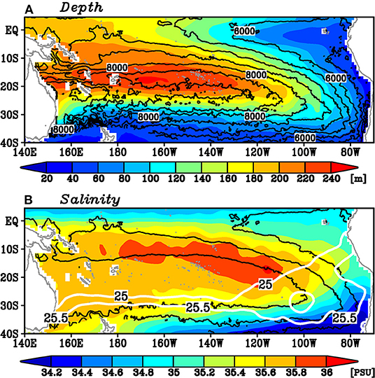
Figure 1. Mean state of (A) the depth (color), the Montgomery potential (kg m−1 s−2; contour), and (B) the salinity (color) of the 25–25.5σθ isopycnals from 2005 to 2018. The contour interval in (A) is 500 kg m−1 s−2 and the contours larger than 10,000 kg m−1 s−2 are not plotted. Black contours in (B) denote 6,000, 7,000, and 8,000 kg m−1 s−2 isopleths of the mean Montgomery potential. White contours in (B) denote the mean outcrop lines of 25 and 25.5σθ in September.
Interestingly, the standard deviations of the spiciness anomalies of these water masses on the 25–25.5σθ isopycnals have different spatial distributions in the raw and the 9-month running mean filtered time series (Figure 2). The former map exhibits a large peak (Figure 2A). In this map, the relation of the spiciness anomaly and the aforementioned interior and the western boundary routes is unclear. On the other hand, the latter map exhibits two peaks on these isopycnals (Figure 2B), although its amplitude is one-third of that of the raw time series peak. Both patterns indicate the large standard deviations in the outcrop region of the 25 and 25.5σθ isopycnals. It is worth noting that the spatial pattern of the standard deviation of spiciness anomalies on these isopycnals has been reported by previous studies (e.g., Kolodziejczyk and Gaillard, 2012; Li et al., 2012), but the two peaks of the low-pass filtered spiciness anomalies have not been reported. In one pathway, the water masses subduct north of 20°S and flow northwestward roughly along the mean Montgomery potential. The water masses along this pathway likely directly enter the equatorial region. In the other pathway, the water masses subduct south of 20°S and flow westward to the western boundary along 15°S, which is also likely aligned with the mean Montgomery potential. These water masses correspond to the salinity maximum on these isopycnals (Figure 1B) as well as the bottom of the South Pacific Tropical Water. The standard deviations of the low-pass filtered salinity of these two pathways are comparable in magnitude.
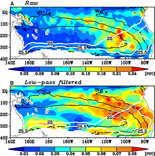
Figure 2. The standard deviation of (A) the raw salinity and (B) the low-pass filtered salinity on the 25–25.5σθ isopycnals. Black contours denote 6,000, 7,000, and 8,000 kg m−1 s−2 isopleths of the mean Montgomery potential. White contours denote the mean outcrop lines of 25 and 25.5σθ in September. The two gray boxes in (B) denote the region where the area-averaged salinity anomalies shown in Figure 4 are calculated.
These two pathways were seen from the meridional section of the low-pass filtered standard deviation of the salinity anomalies on the isopycnals averaged between 140°W and 180° (Figure 3). The peak of the northern pathway extends to the surface layer, while the maximum of the standard deviation shifts southward in a shallower layer. In contrast, the peak corresponding to the southern pathway is confined between the 25 and 25.5σθ isopycnals. The minimum of the standard deviation on these isopycnals is located along 10°S. In summary, we found two pathways from the subtropics to the tropics. Hereafter, we refer to the former as the northern pathway and the latter as the southern pathway. These two pathways are likely related to the interior route and western boundary route.
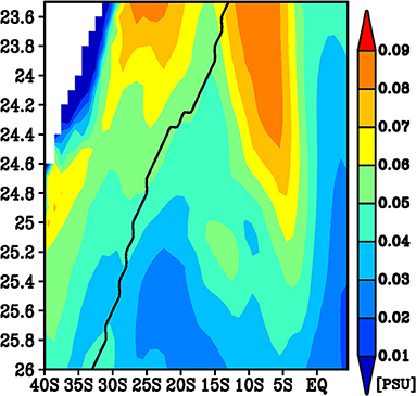
Figure 3. A density latitude diagram of the standard deviation of the low-pass filtered salinity on the isopycnals averaged 140°W−180°. The black line indicates that the mean outcrop line in September.
The variations of the low-pass filtered spiciness anomalies are largely independent between the two pathways. Figure 4 shows the raw and the low-pass filtered time series of the spiciness anomalies averaged around the outcrop line of the 25σθ isopycnal (see Figure 2B). The correlation coefficient between these two time series is not statistically significant 90% confidence level (p = 0.44). The spiciness anomalies in the northern pathway decreased (cooling and freshening) from 2005 to 2009 and then turned to an upward trend to the end of the data. On the other hand, the spiciness anomalies of the southern pathway showed an upward trend with interannual and decadal variability. The detailed features of these spiciness variations will be discussed in later subsections.
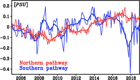
Figure 4. Salinity anomalies on the 25–25.5σθ isopycnals averaged over 17.5°-22.5°S, 105°-115°W (blue) and 12.5°-17.5°S, 90°-100°W (red). The thin and thick lines are the raw and a 9 month running mean filtered time series, respectively.
The fundamental question is the cause of these two paths. In other words, what kinds of processes are essential to separate these two pathways? The salinity variability on the isopycnals shows the minimum along 10°S. This zonally elongated structure suggests the importance of ocean currents, which tend to have zonal jet structures in this area (Kessler and Gourdeau, 2006). Figures 5A,B shows the surface zonal velocity by the OSCAR dataset and the surface zonal geostrophic velocity based on the MDOT dataset, respectively, in the western South Pacific. The surface zonal velocities of both datasets indicate the eastward current along 10°S, while its eastern extent is somewhat different between the two datasets. The eastward current along 10°S based on the MDOT dataset extends to 140°W. On the other hand, the eastward current of the OSCAR dataset extends only to 170°W. This discrepancy might be due to the difference of spatial resolution between the two datasets. This eastward current is the South Equatorial Countercurrent (SECC; e.g., Ganachaud et al., 2014). The mechanism of this surface zonal current can be explained by the Sverdrup current (Chen and Qiu, 2004). This surface eastward current extends to the subsurface. On the 25–25.5σθ isopycnals, the eastward current is also found along 10°S (Figure 5C), although its strength becomes weaker and the spatial structure is somewhat noisy.
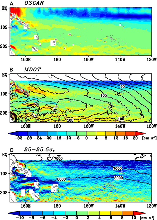
Figure 5. Mean state of (A) the surface zonal velocity by the OSCAR dataset, (B) the surface zonal geostrophic velocity (color) and the contour of the sea surface height (contour) of the MDOT dataset, and (C) the zonal geostrophic velocity on the 25–25.5σθ isopycnals along with the 7,000 and 8,000 kg m−1 s−2 isopleths of the mean Montgomery potential (contour). In (B,C), the zonal velocity is not plotted north of 3°S.
A comparison between Figure 2B and Figure 5C indicates that the location of SECC is consistent with the weak standard deviation of the low-pass filtered spiciness anomalies on the 25–25.5σθ isopycnals. One can anticipate that the westward advection of spiciness anomalies on the isopycnals was prevented by the eastward current. To test this idea, we perform a simple passive tracer experiment. Figure 6A shows the initial condition of the passive tracers, where the passive tracers were placed at a 0.1° interval in both zonal and meridional directions. These tracers are passively advected by the climatological geostrophic current on the 25–25.5σθ isopycnals for 4 years. This selection of 4-year is because spiciness anomalies are attenuated during the migration (e.g., Sasaki et al., 2010). The mean geostrophic current sets zero north of 3°S, because the geostrophic balance is not valid near the equator. However, because our focus of this passive tracer experiment is the locations of the tracers around 10°S, this setting does not significantly influence the experiment result.
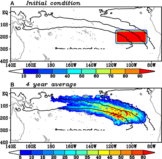
Figure 6. (A) Initial condition and (B) 4-year average of passive tracer concentrations (color) on the 25–25.5σθ isopycnals along with the 6,000, 7,000, and 8,000 kg m−1 s−2 isopleths of the mean Montgomery potential (contour).
Figure 6B shows the mean locations of the passive tracers of the 4-year experiment. Results below are robust if a 3 or a 5-year experiment is performed. The location of the passive tracers has two peaks, which is similar to the standard deviation of the low-pass filtered spiciness anomalies (Figure 2B). The minimum between these two peaks is located along 10°S, consistent with the location of SECC (Figure 5). This result implies that it takes time spiciness anomalies to enter the SECC region. Therefore, SECC prevents the spiciness anomaly advection from the subtropics to the tropics.
The difference between the raw and low-pass filtered spiciness anomalies is likely because the advection process acts as a low-pass filter to spiciness anomalies (Kilpatrick et al., 2011). That is, in the region where the advection process is important, the low-pass filtered standard deviation is large. This idea is consistent with the result that SECC prevents the intrusion of the passive tracers along 10°S (Figure 6B), where the standard deviation of the low-pass filtered salinity exhibits the local minimum (Figure 2B). High-frequent signals caused by, for example, anomalous advection of the climatological spiciness gradient, are damped by the advection.
This subsection will examine the variability of the spiciness anomalies in the southern pathway to investigate its relation to the western boundary route. Since the large standard deviations of the low-pass filtered salinity of this pathway are roughly aligned with the Montgomery potential (Figure 2B), we begin to investigate the variability of the southern pathway along the stream line. Figure 8 shows the time-longitude diagram of the low-pass filtered salinity anomalies along the southern pathway on the 25–25.5σθ. This diagram indicates clear westward propagation of the spiciness anomalies extending to the western boundary region. This is consistent with the advection of the mean geostrophic current on the isopycnals (e.g., Sasaki et al., 2010). The mean zonal velocity along 10°S is about 0.1 m s−1 (Figure 5C). Thus, it takes about 3 years to traverse the 9,000 km (roughly from 100°W to 170°E). The decay of the spiciness anomalies along the propagation seems relatively weak. As mentioned above, this path flows along the salinity maximum on the isopycnals and the bottom of the South Pacific Tropical Water. A similar westward propagation signal along the salinity maximum on the 24–25σθ isopycnals has been reported by Zhang and Qu (2014), although the amplitude of the salinity anomalies in the present study is 2–3 times larger than that of Zhang and Qu (2014; see their Figure 3C).
An interesting feature in Figure 8 is the upward trend of the salinity (and temperature) anomalies, as mentioned in Section The Overall Pattern of Spiciness Variability. To clarify the spatial structure of this upward trend, Figure 7A shows the linear trend of the salinity on the 25–25.5σθ isopycnals from 2005 to 2018, where these trends and their statistical significance are estimated without the low-pass filtering not to reduce the degrees of freedom. The statistically significant upward trend of the salinity is found in the outcrop region and extends to westward along the mean Montgomery potential. The amplitude of the trend is larger in the more upstream region. These features are consistent with the westward advection of the spiciness anomalies by the mean geostrophic current. The vertical structures of the trend along 140°W indicate that the upward trend is located between the 24.5 and 25.6σθ isopycnals with a peak at 25.2σθ (not shown), consistent with the large standard deviation of the low-pass filtered spiciness anomalies there (Figure 3). Note that a closer look at the variability in the downstream region west of 180° in Figure 8 shows that the spiciness anomalies in this region are positive during 2005–2006, and thus their linear trend is not statistically significant (Figure 7A). This implies that the upward trend of the spiciness anomalies along the southern pathway might be a part of decadal or interdecadal variability.
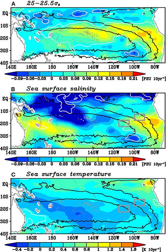
Figure 7. Linear trends of (A) the salinity on the 25–25.5σθ isopycnals, (B) the sea surface salinity, and (C) the sea surface temperature. White contours denote the regions where the trends are significant at 90% confidence level. Black contours denote 6,000, 7,000, and 8,000 kg m−1 s−2 isopleths of the mean Montgomery potential. The two gray boxes in (B,C) denote the region where the area-averaged salinity anomalies shown in Figure 4 are calculated.
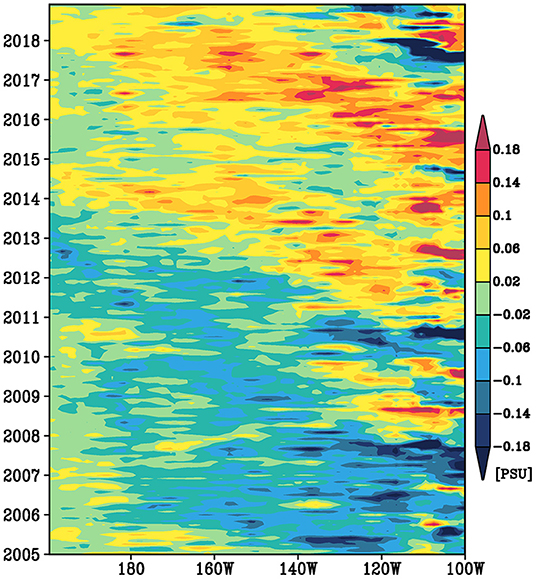
Figure 8. A time-longitude diagram of the low-pass filtered salinity anomaly averaged vertically over the 25–25.5σθ isopycnals and meridionally over the 8,000 and 8,500 kg m−1 s−2 mean Montgomery potential isopleths.
This subsection will examine the spiciness anomalies along the northern pathway to examine their equatorward propagation. This pathway is similar to the spiciness signal propagation reported by Li et al. (2012). Li et al. (2012) determined the propagation pathway by the mean acceleration potential. However, the mean acceleration potential might not be suitable close to the equator, because the geostrophic balance is no longer valid there. In this study, to objectively identify the pathway of the signals, we performed the lag correlation analysis. This is an advantage to use a longer observational dataset compared to the previous studies. The time series of the salinity anomalies on the 25–25.5σθ isopycnals average over 12.5–17.5°S, 105–115°W (red line in Figure 4) is used as a representative time series of the spiciness variability in the upstream region of the northern pathway.
The lag correlation analysis can capture the equatorward advection of the spiciness anomalies along the northern pathway (Figure 9). Initially, the correlation was statistically significant around the outcrop region (Figure 9A). These significant correlation coefficients migrated northwestward along the mean Montgomery potential (Figure 9B). Then, they moved equatorward and entered the equatorial region (Figure 9C), although their trajectory somewhat deviated east from the mean Montgomery potential. The maximum correlation coefficients are still larger than 0.8. It takes about 2 years from the outcrop region to the equatorial region. Note that similar equatorward propagation of the spiciness anomalies can be seen from the correlation map using the detrended time series (not shown) (L235–236).
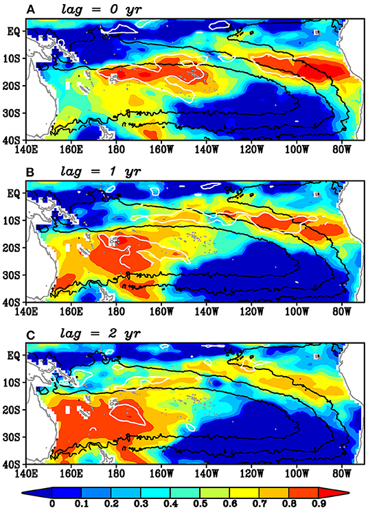
Figure 9. Lag correlation coefficients of the low-pass filtered salinity on the 25–25.5σθ isopycnals onto the low-pass filtered salinity anomalies on the 25–25.5σθ isopycnals averaged over the upstream region (12.5°-17.5°S, 90°-100°W; red thick line in Figure 4) for the lag years of (A) 0, (B) 1, and (C) 2, where positive lag means that the salinity in the upstream region leads. White contours denote the regions where the correlations are significant at 90% confidence level. Black contours denote 6,000, 7,000, and 8,000 kg m−1 s−2 isopleths of the mean Montgomery potential.
The time-latitude diagram along the northern pathway confirms an equatorward advection of the spiciness anomalies (Figure 10). In the upstream region, the salinity anomalies on the 25–25.5σθ isopycnals were negative from 2005 to 2012 and positive after 2012. These spiciness anomalies are advected equatorward. Before the arrival of the negative salinity anomalies, the salinity anomalies were positive in the equatorial region. The decay of the amplitude of the spiciness anomalies during the equatorward propagation is likely weak.
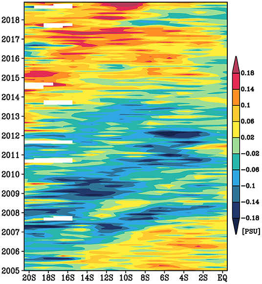
Figure 10. A time-latitude diagram of the low-pass filtered salinity anomaly averaged vertically over the 25–25.5σθ isopycnals and zonally over the 6,000 and 6,500 kg m−1 s−2 mean Montgomery potential isopleths.
Finally, the relation between the spiciness variability of the northern pathway and temperature and salinity variations around the outcrop region is investigated. To this end, we also examined the correlation coefficients of the representative time series of the spiciness variability in the upstream region of the northern pathway to the sea surface properties in the outcrop region. The results showed that the spiciness anomalies along the northern pathway are related to sea surface salinity variability, but not sea surface temperature variability (not shown). This result is similar to the result of the southern pathway (Figure 7).
We examined the subduction and migration of the spiciness anomalies on the 25–25.5σθ isopycnals in the subtropical gyre of the South Pacific from 2005 to 2018 using the observational dataset. We revealed that the low-pass filtered spiciness anomalies follow two pathways from the subtropical region to the tropical region on these isopycnals (Figures 2B, 3). We referred to these two pathways as the northern pathway and the southern pathway. From the viewpoint of the connection between the subtropics and the tropics, the northern and southern pathways are related to the interior and western boundary routes, respectively. The passive tracer experiment revealed that the advection by SECC divides these two pathways (Figures 5, 6). Hence, SECC plays a key role in determining whether a spiciness anomaly propagates through the interior route or the western boundary route.
In the southern pathway, the water masses, which correspond to the salinity maximum on these isopycnals (Figure 1B) as well as the bottom of the South Pacific Tropical Water, subducted south of 20°S and mainly flowed westward via the mean geostrophic current to the western boundary region (Figure 8). Positive temperature and salinity trends were prominent along this pathway during the study period (Figure 7A). Interestingly, the sea surface salinity showed a similar upward trend in the outcrop region (Figure 7B), although the sea surface temperature did not (Figure 7C). The trend of the sea surface salinity in this region is comparable in magnitude to the trend of the salinity anomalies on the 25–25.5σθ isopycnals (Figure 7A). These results suggest that the trend of the sea surface salinity contributes to the upward trend along the southern pathway. It is worth noting that the trend of the sea surface salinity was confined in the outcrop region and did not extend westward. On the other hand, the water masses subduct north of 20°S and go directly to the tropics through the interior region in the northern pathway (Figures 9, 10). Decadal variability of the spiciness anomalies is prominent along this pathway. The sea surface salinity variability is likely important for generating the spiciness anomalies on the isopycnals in this pathway.
An important implication of our study is that a spatial pattern of low-frequent variability of spiciness anomalies reflects detailed ocean circulation on isopycnals. This result means that we can obtain the information of subsurface ocean circulation only from temperature and salinity observations without the assumption of geostrophy. In addition, to investigate a spatial structure of low-frequent spiciness variability from a numerical model is a useful benchmark to evaluate simulated subsurface circulation, such as the connection from the subtropics to the tropics in the present study.
Publicly available datasets were analyzed in this study. This data can be found at: The MOAA GPV dataset was downloaded from the JAMSTEC website (ftp://ftp2.jamstec.go.jp/pub/argo/MOAA_GPV/). The OSCAR dataset was obtained from JPL Physical Oceanography DAAC (https://podaac.jpl.nasa.gov/dataset/OSCAR_L4_OC_third-deg). The MDOT dataset was provided by Asia-Pacific Data Research Center (http://apdrc.soest.hawaii.edu/datadoc/mdot.php). The sea level anomaly data were obtained from the CMEMS website (https://marine.copernicus.eu/).
YS and YI did initial analysis. YS continued the analysis and summarized the final manuscript. Both authors contributed to the article and approved the submitted version.
This research was supported by the Japan Society for the Promotion of Science (JSPS) KAKENHI Grants 16K1780 and 19H05704, which is funded by the Ministry of Education, Culture, Sports, Science, and Technology of Japan.
The authors declare that the research was conducted in the absence of any commercial or financial relationships that could be construed as a potential conflict of interest.
All claims expressed in this article are solely those of the authors and do not necessarily represent those of their affiliated organizations, or those of the publisher, the editors and the reviewers. Any product that may be evaluated in this article, or claim that may be made by its manufacturer, is not guaranteed or endorsed by the publisher.
We thank Profs. S. Minobe and M. Inatsu for valuable comments.
Bonjean, F., and Lagerloef, G. S. E. (2002). Diagnostic model and analysis of the surface currents in the tropical Pacific ocean. J. Phys. Oceanogr. 32, 2938–2954. doi: 10.1175/1520-0485(2002)032<2938:DMAAOT>2.0.CO;2
Chen, S., and Qiu, B. (2004). Seasonal variability of the South Equatorial Countercurrent. J. Geophys. Res. 109:C08003. doi: 10.1029/2003JC002243
Cushman-Roisin, B. (1994). Introduction to Geophysical Fluid Dynamics. Princeton, NJ: Prentice Hall, 320.
Fukumori, I., Lee, T., Cheng, B., and Menemenlis, D. (2004). The origin, pathway, and destination of Niño-3 water estimated by a simulated passive tracer and its adjoint. J. Phys. Oceanogr. 34, 582–604. doi: 10.1175/2515.1
Ganachaud, A., Cravatte, S., Melet, A., Schiller, A., Holbrook, N. J., Sloyan, B. M., et al. (2014). The Southwest Pacific Ocean circulation and climate experiment (SPICE). J. Geophys. Res. 119, 7660–7686. doi: 10.1002/2013JC009678
Gu, D. F., and Philander, S. G. H. (1997). Interdecadal climate fluctuations that depend on exchanges between the Tropics and extratropics. Science 275, 805–807. doi: 10.1126/science.275.5301.805
Hosoda, S., Ohira, T., and Nakamura, T. (2008). A monthly mean dataset of global oceanic temperature and salinity derived from Argo float observations. JAMSTEC Rep. Res. Dev. 8, 47–59. doi: 10.5918/jamstecr.8.47
Kaplan, D., and Glass, L. (1995). Understanding Nonlinear Dynamics. New York, NY: Springer-Verlag. p. 420. doi: 10.1007/978-1-4612-0823-5
Kessler, W. S., and Gourdeau, L. (2006). Wind-driven zonal jets in the South Pacific Ocean. Geophys. Res. Lett. 33:L03608. doi: 10.1029/2005GL025084
Kilpatrick, T., Schneider, N., and Di Lorenzo, E. (2011). Generation of Low-frequency spiciness variability in the thermocline. J. Phys. Oceanogr. 41, 365–377. doi: 10.1175/2010JPO4443.1
Kolodziejczyk, N., and Gaillard, F. (2012). Observation of spiciness interannual variability in the Pacific pycnocline. J. Geophys. Res. 117:C12018. doi: 10.1029/2012JC008365
Kouketsu, S., Osafune, S., Kumamoto, Y., and Uchida, H. (2017). Eastward salinity anomaly propagation in the intermediate layer of the North Pacific. J. Geophys. Res. 122, 1590–1607. doi: 10.1002/2016JC012118
Lee, T., and Fukumori, I. (2003). Interannual-to-decadal variations of tropical-subtropical exchange in the pacific ocean: boundary versus interior pycnocline transports. J. Clim. 16, 4022–4042. doi: 10.1175/1520-0442(2003)016<4022:IVOTEI>2.0.CO;2
Li, Y., Wang, F., and Sun, Y. (2012). Low-frequency spiciness variations in the tropical Pacific Ocean observed during 2003-2012. Geophys. Res. Lett. 39:L23601. doi: 10.1029/2012GL053971
Liu, Z. (1999). Forced planetary wave response in a thermocline gyre. J. Phys. Oceanogr. 29, 1036–1055. doi: 10.1175/1520-0485(1999)029<1036:FPWRIA>2.0.CO;2
Maximenko, N., Niiler, P., Rio, M.-H., Melnichenko, O., Centurioni, L., Chambers, D., et al. (2009). Mean dynamic topography of the ocean derived from satellite and drifting buoy data using three different techniques. J. Atmos. Ocean. Technol. 26, 1910–1919. doi: 10.1175/2009JTECHO672.1
McCreary, J. P., and Lu, P. (1994). Interaction between the subtropical and equatorial ocean circulations: the subtropical cell. J. Phys. Oceanogr. 24, 466–497. doi: 10.1175/1520-0485(1994)024<0466:IBTSAE>2.0.CO;2
Nagura, M., and Kouketsu, S. (2018). Spiciness anomalies in the upper South Indian Ocean. J. Phys. Oceanogr. 48, 9, 2081–2101. doi: 10.1175/JPO-D-18-0050.1
Nonaka, M., and Sasaki, H. (2007). Formation mechanism for isopycnal temperature-salinity anomalies propagating from the Eastern South Pacific to the Equatorial Region. J. Clim. 20, 1305–1315. doi: 10.1175/JCLI4065.1
Nonaka, M., and Xie, S.-P. (2000). Propagation of North Pacific interdecadal subsurface temperature anomalies in an ocean GCM. Geophys. Res. Lett. 27, 3747–3750. doi: 10.1029/2000GL011488
Ogata, T., and Nonaka, M. (2020). Mechanisms of long-term variability and recent trend of salinity along 137°E. J. Geophys. Res. 125:2. doi: 10.1029/2019JC015290
Pierce, D. W., Barnett, T. B., and Latif, M. (2000). Connections between the Pacific Ocean Tropics and midlatitudes on decadal timescales. J. Clim. 13, 1173–1194. doi: 10.1175/1520-0442(2000)013<1173:CBTPOT>2.0.CO;2
Qiu, B., and Huang, R. X. (1995). Ventilation of the North Atlantic and North Pacific -subduction versus obduction. J. Phys. Oceanogr. 25, 2374–2390. doi: 10.1175/1520-0485(1995)025<2374:VOTNAA>2.0.CO;2
Qu, T., Gao, S., Fukumori, I., Fine, R. A., and Lindstrom, E. J. (2008). Subduction of South Pacific waters. Geophys. Res. Lett. 35:L02610. doi: 10.1029/2007GL032605
Qu., T., Gao, S., and Fine, R. A. (2013). Subduction of South Pacific tropical water and its equatorward pathways as shown by a simulated passive tracer. J. Phys. Oceanogr. 43, 1551–1565. doi: 10.1175/JPO-D-12-0180.1
Santer, B. D., Wigley, T. M. L., Boyle, J. S., Gaffen, D. J., Hnilo, J. J., Nychka, D., et al. (2000). Statistical significance of trends and trend differences in layer-average atmospheric temperature time series. J. Geophys. Res. 105, 7337–7356. doi: 10.1029/1999JD901105
Sasaki, Y. N., Schneider, N., Maximenko, N., and Lebedev, K. (2010). Observational evidence for propagation of decadal spiciness anomalies in the North Pacific. Geophys. Res. Lett. 37:L07708. doi: 10.1029/2010GL042716
Schneider, N., Miller, A. J., Alexander, M. A., and Deser, C. (1999). Subduction of decadal North Pacific temperature anomalies: observations and dynamics. J. Phys. Oceanogr. 29, 1056–1070. doi: 10.1175/1520-0485(1999)029<1056:SODNPT>2.0.CO;2
Taguchi, B., and Schneider, N. (2014). Origin of decadal-scale, eastward-propagating heat content anomalies in the North Pacific. J. Clim. 27, 7568–7586. doi: 10.1175/JCLI-D-13-00102.1
Tsuchiya, M., and Talley, L. D. (1996). Water-property distributions along an eastern Pacific hydrographic section at 135W. J. Mar. Res. 54, 541–564. doi: 10.1357/0022240963213583
Yeager, S. G., and Large, W. G. (2004). Late-winter generation of spiciness on subducted isopycnals. J. Phys. Oceanogr. 34, 1528–1547. doi: 10.1175/1520-0485(2004)034<1528:LGOSOS>2.0.CO;2
Zeller, M., McGregor, S., van Sebille, E., Capotondi, A., and Spence, P. (2021). Subtropical-tropical pathways of spiciness anomalies and their impact on equatorial Pacific temperature. Clim. Dyn. 56, 1131–1144. doi: 10.1007/s00382-020-05524-8
Keywords: spiciness anomaly, subduction, decadal variability, South Equatorial Countercurrent, Argo
Citation: Sasaki YN and Iwai Y (2022) Two Pathways of Subsurface Spiciness Anomalies in the Subtropical South Pacific. Front. Clim. 4:897498. doi: 10.3389/fclim.2022.897498
Received: 16 March 2022; Accepted: 16 May 2022;
Published: 02 June 2022.
Edited by:
Tomomichi Ogata, Japan Agency for Marine-Earth Science and Technology (JAMSTEC), JapanReviewed by:
Jasti S. Chowdary, Indian Institute of Tropical Meteorology (IITM), IndiaCopyright © 2022 Sasaki and Iwai. This is an open-access article distributed under the terms of the Creative Commons Attribution License (CC BY). The use, distribution or reproduction in other forums is permitted, provided the original author(s) and the copyright owner(s) are credited and that the original publication in this journal is cited, in accordance with accepted academic practice. No use, distribution or reproduction is permitted which does not comply with these terms.
*Correspondence: Yoshi N. Sasaki, c2FzYWtpeW9Ac2NpLmhva3VkYWkuYWMuanA=; orcid.org/0000-0003-2321-5365
Disclaimer: All claims expressed in this article are solely those of the authors and do not necessarily represent those of their affiliated organizations, or those of the publisher, the editors and the reviewers. Any product that may be evaluated in this article or claim that may be made by its manufacturer is not guaranteed or endorsed by the publisher.
Research integrity at Frontiers
Learn more about the work of our research integrity team to safeguard the quality of each article we publish.