How Climate Extremes Influence Conceptual Rainfall-Runoff Model Performance and Uncertainty

Watson, Andrew; Midgley, Guy; Ray, Patrick; Kralisch, Sven; Helmschrot, Jörg

doi:10.3389/fclim.2022.859303

ORIGINAL RESEARCH article

Front. Clim., 22 June 2022

Sec. Climate Risk Management

Volume 4 - 2022 | https://doi.org/10.3389/fclim.2022.859303

This article is part of the Research Topic From Observations to Predictions and Projections: Opportunities and Challenges for Climate Risk Assessment and Management in Sub-Saharan Africa View all 10 articles

How Climate Extremes Influence Conceptual Rainfall-Runoff Model Performance and Uncertainty

$\nAndrew Watson,$ Andrew Watson^1,2^*

Guy Midgley^2,3

Patrick Ray⁴

Sven Kralisch⁵

Jörg Helmschrot^1,6

¹Stellenbosch University Water Institute, Stellenbosch University, Stellenbosch, South Africa
²School for Climate Studies, Stellenbosch University, Stellenbosch, South Africa
³Global Change Biology Group, Department of Botany and Zoology, Stellenbosch University, Stellenbosch, South Africa
⁴Department of Chemical and Environmental Engineering, University of Cincinnati, Cincinnati, OH, United States
⁵Department of Geoinformation Science, Friedrich-Schiller-University Jena, Jena, Germany
⁶Institute of Meteorology and Climate Research, Karlsruhe Institute of Technology, Karlsruhe, Germany

Rainfall-runoff models are frequently used for assessing climate risks by predicting changes in streamflow and other hydrological processes due to anticipated anthropogenic climate change, climate variability, and land management. Historical observations are commonly used to calibrate empirically the performance of conceptual hydrological mechanisms. As a result, calibration procedures are limited when extrapolated to novel climate conditions under future scenarios. In this paper, rainfall-runoff model performance and the simulated catchment hydrological processes were explored using the JAMS/J2000 model for the Berg River catchment in South Africa to evaluate the model in the tails of the current distribution of climatic conditions. An evolutionary multi-objective search algorithm was used to develop sets of parameters which best simulate “wet” and “dry” periods, providing the upper and lower bounds for a temporal uncertainty analysis approach to identify variables which are affected by these climate extremes. Variables most affected included soil-water storage and timing of interflow and groundwater flow, emerging as the overall dampening of the simulated hydrograph. Previous modeling showed that the JAMS/J2000 model provided a “good” simulation for periods where the yearly long-term mean precipitation shortfall was <28%. Above this threshold, and where autumn precipitation was reduced by 50%, this paper shows that the use of a set of “dry” parameters is recommended to improve model performance. These “dry” parameters better account for the change in streamflow timing of concentration and reduced peak flows, which occur in drier winter years, improving the Nash-Sutcliffe Efficiency (NSE) from 0.26 to 0.60 for the validation period 2015–2018, although the availability of climate data was still a potential factor. As the model performance was “good” (NSE > 0.7) during “wet” periods using parameters from a long-term calibration, “wet” parameters were not recommended for the Berg River catchment, but could play a large role in tropical climates. The results of this study are likely transferrable to other conceptual rainfall/runoff models, but may differ for various climates. As greater climate variability drives hydrological changes around the world, future empirically-based hydrological projections need to evaluate assumptions regarding storage and the simulated hydrological processes, to enhanced climate risk management.

Introduction

The frequency, duration and intensity of droughts around the world are increasing, resulting in the widespread loss of natural vegetation and wildlife, economic instability and increases in anthropogenic water use (IPCC, 2021). While in some situations, specific regions have benefitted in terms of more favorable climates for crop growth and enhanced carbon dioxide fertilization (Bond and Midgley, 2012), meteorological shortfalls and the intensification of dry periods will impact many vulnerable regions which do not have the economic ability to adapt (Collier et al., 2008; Allison et al., 2009). The expectation is that precipitation variability, exaggerated by increasing temperatures and resulting evapotranspiration, will plague many parts of Africa for the unforeseen future (Engelbrecht and Monteiro, 2021). The Western Cape (WC) of South Africa has been subject to an increased meteorological drought frequency (1–3 years: Watson et al., 2022) and recently experienced an intense drought between 2015 and 2018, where reservoir levels collectively dropped to a low of 17% (DWS, 2018). Research has mainly focused on the mechanisms affecting local precipitation (Wilks, 2011), characterizing the meteorological (Archer et al., 2019) and agricultural drought (Watson et al., 2022). While recent climate change projections have been developed for Africa (Haensler, 2010; Haensler et al., 2011; Archer et al., 2018; Weber, 2018; Lim Kam Sian et al., 2021; Majdi et al., 2022), their bearing on local hydrological condition and function affect the development of appropriate adaptation strategies and the rate at which Africa acts to reduce the effects of global warming (Kusangaya et al., 2014). Furthermore, uncertainty still remains whether hydrological models can reproduce hydrological flows considering future non-stationary climatic conditions, which has been an issue for rainfall-runoff model applications around the world (Deb and Kiem, 2020; Fowler et al., 2020).

SWAT (Arnold et al., 1998), a common conceptual rainfall-runoff model, has been used as a predictive tool to assess the impact of different climate change projections on the future water resource availability in different African settings (Akoko et al., 2021; Chomba et al., 2021; Maviza and Ahmed, 2021; Osman et al., 2021). Using historical conditions, hydrological process simulations for rainfall-runoff models have been calibrated with historical streamflow measurements and other hydroclimatic observations. Accounting for additional spatial variables has improved rainfall-runoff model performance and the overall inclusion of different hydrological processes (Vaze et al., 2011; Khakbaz et al., 2012). Furthermore, the advancement of rainfall-runoff modeling into fully automated calibration procedures such as the use of the Non-dominated Sorting Genetic Algorithm (NSGA-II: Deb et al., 2002) and parameter uncertainty analysis such as the Monte Carlo Analysis (MCA: Hornberger and Spear, 1981), criteria-based performance assessments (Krause and Boyle, 2005), Generalized Likelihood Uncertainty Estimation (GLUE: Beven and Binley, 1992), and Dynamic Identifiability Analysis (DYNIA: Wagener et al., 2002) has improved hydrological model applications around the world. Although physical inputs (e.g., climate, topography, soil, hydrogeology, and land use) form spatial inputs in most distributed rainfall-runoff models (e.g., SWAT: Arnold et al., 1998; J2000: Krause, 2001, PRMS/MMS: Leavesley et al., 1996), conceptual and empirical parameters which are often calibrated based on streamflow measurements, are impacted by non-stationary climate conditions (Deb and Kiem, 2020) and complex hydrological processes are often inferred from only river flow measurements (Jakeman and Hornberger, 1993). As a result, recent concerns have been raised about the ability of “bucket” type rainfall-runoff models in reproducing hydrological conditions under future projections and in particular how these methods assume long-term stationary storage conditions (Fowler et al., 2020).

In this study, the performance of the JAMS/J2000 rainfall-runoff model was assessed during periods of climate extremes between 1984 and 2018 for the Berg River catchment in South Africa (Figure 1). The different climate extremes were distinguished using the Soil Moisture Deficit Index (SMDI: Narasimhan and Srinivasan, 2005; Watson et al., 2022) into periods of “wet” and “dry”. Yearly average values of 1> SMDI <−1 were used to differentiate between “wet” and “dry” years. The NSGA-II (Deb et al., 2002), an evolutionary multi-objective search algorithm was used to develop sets of parameters which “best” simulate “wet” and “dry” periods for the JAMS/J2000 model of the Berg River. To identify parameters which may vary in both space and time, as a function of a change in hydroclimatic and other biophysical processes, DYNIA (Wagener et al., 2002) was used. Further to the temporal uncertainty of different parameters across “wet” and “dry” periods, we aim to demonstrate the extent of climatic disturbance with which a single parameter set can simulate catchment hydrological processes within a certain degree of efficiency. As unstable climate conditions begin to affect conceptual assumptions regarding soil water and aquifer storage, as well as water use behavioral changes within the system, understanding temporal parameter variability is required to develop more dynamic rainfall-runoff models which are required for climate change-based assessments.

FIGURE 1

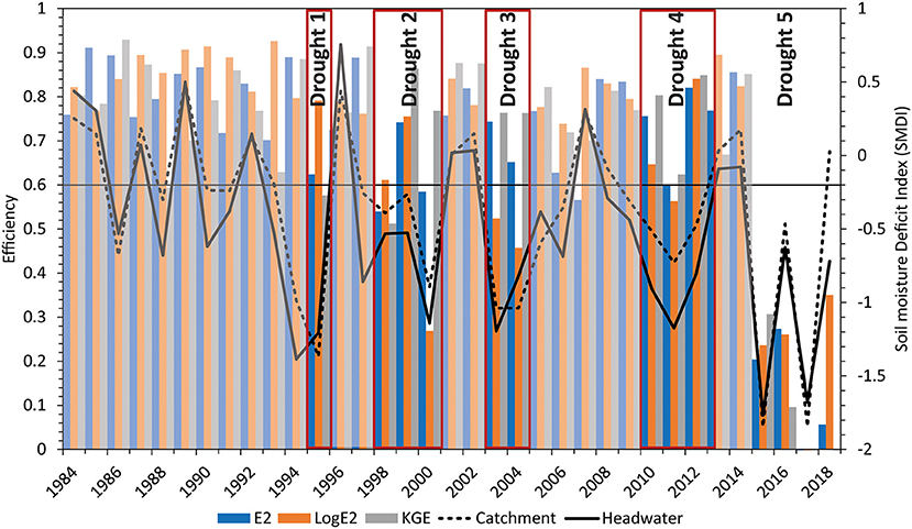
Figure 1. The long-term (1984–2018) efficiency of the JAMS/J2000 model for the Berg River catchment (after Watson et al., 2022), represented as the yearly Nash–Sutcliffe [NSE; Nash, 1970] efficiency in standard form (E2) and logarithmic form (logE2) as well as with the Kling- Gupta efficiency (KGE). The simulated Soil Moisture Deficit Index (SMDI) for the Berg River catchment (black dashed line) and headwater (black line), indicating a reduce performance during “dry” periods when the simulated SMDI was < −0.5.

Environmental Setting

The Berg River is a meso-scale catchment with an extent of 7,700 km², which is located on the West coast, South Africa (Figure 2). The catchment supports a large agricultural sector (Claassen, 2015), used in inter-basin water supply (Muller, 2002), as well as hosting an ecologically significant estuary (Sinclair et al., 1984). The catchment falls within the Cape Fold Belt, a thrust belt which resulted in the formation of a sequence of sedimentary rock layers known as the Cape Supergroup (Johnson et al., 2006). The catchment drains the Hottentots-Holland and Haweqwa Mountains, which receive the bulk of precipitation with a maximum of 3,198 mm/annum and are hosted by the Cambrian Table Mountain Group sandstones (TMG) in the Southern tip of the catchment. The TMG is widely known as a highly productive secondary fractured rock aquifer with estimated recharge values of between 13 and 27% of Mean Annual Precipitation (MAP) (Weaver and Talma, 2005; Wu, 2005; Miller et al., 2017). Precipitation reduces to 700–800 mm/annum near the town of Paarl, where an alluvial aquifer is often thick (15–20 m) and underlain by the Malmesbury Group shales (MG). Groundwater recharge rates for the alluvial aquifer are between 0.2 and 3.4% (Conrad et al., 2004), but as much as 6% of MAP (Vetger, 1995) while less is known about recharge rates for the MG.

FIGURE 2

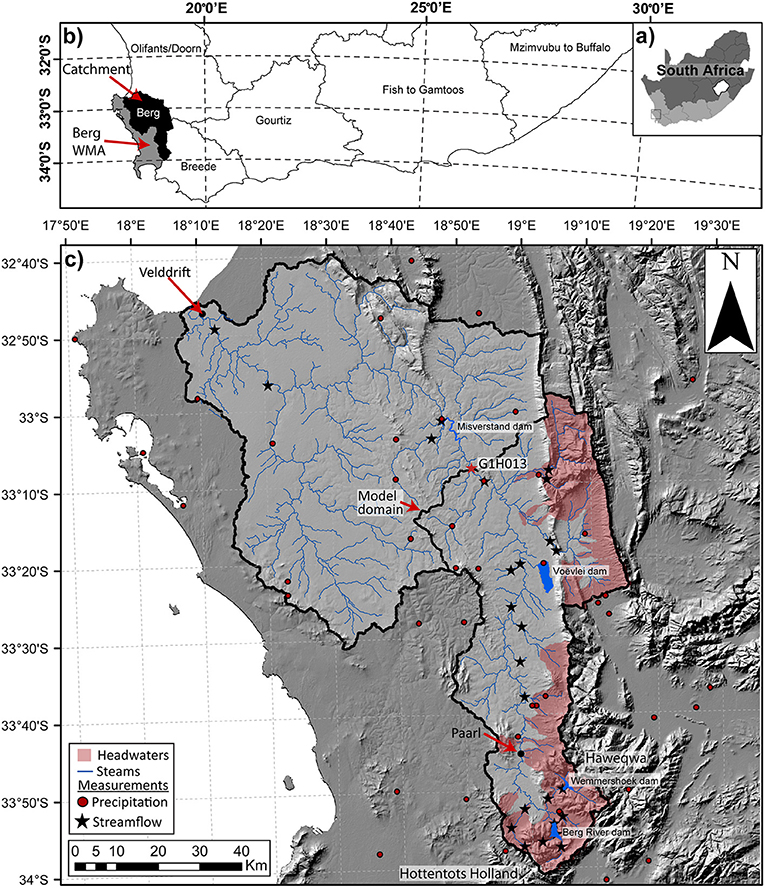
Figure 2. (a) Location of the Western Cape (WC) within South Africa, (b) Berg River Water Management Area (WMA) surrounded by other WMA's within the WC (Breede, Olifants/doorn), (c) Berg River catchment showing locations of precipitation stations (red points), streamflow monitoring (black star), G1H013 gauge (red-star), the modeling domain and locations of major towns, reservoirs (Berg River, Wemmershoek, Voëlvlei and Misverstand dams), the major town of Paarl in context with the mountain ranges of the Hawequa and Hottentots Holland and headwater areas (>300 M A.S.L: red polygon).

Precipitation reduced to 300–400 mm/annum toward Velddrif at the catchment outlet (Lynch, 2004), where the river flows into the Atlantic ocean. Major reservoirs are present in the catchment headwaters (Berg River, Wemmershoek and Voëlvlei dams: 130 (Million) Mm³, 58, and 164 Mm³, respectively), as well as downstream of these reservoirs on the main river channel (Misverstand dam: 8 Mm³). Other significant reservoirs (Theewaterskloof dam: 480 Mm³, Steenbras dam: 33 Mm³, Clanwilliam dam: 121 Mm³) in the Breede and Olifants/doorn Water Management Areas (WMAs), comprise the bulk surface water supply sources in the area.

Precipitation in the Berg River and much of the Mediterranean winter precipitation parts of the WC, is generally received in the months June, July August (JJA) with 50%, followed by March, April, May (MAM) with 23% of the total yearly amount (Watson et al., 2022). September, October, November (SON) and December, January, February (DJF) make up the remaining 19 and 8% of the yearly precipitation amounts. As a result, streamflow is mainly generated JJA, with 61% of the total flow, followed by the SON, MAM, and DJA months with 26, 9, and 4%, respectively (Watson et al., 2022). The temporal variability of MAP within the region, over the last 34 years (1984–2018), shows a higher degree of variability for valley regions (51% of valley MAP) compared with headwater areas (34% of headwater MAP) (Watson et al., 2022). Meteorological droughts have been mostly associated with shortfalls in MAM precipitation (Archer et al., 2019; Watson et al., 2022) (years 2000, 2015, and 2017) but for the drought years: 1994, 2004, and 2011 <50% was received in DJF (Table 1). In 1997 and 2003 meteorological drought was mainly caused by shortfalls in SON and JJA, respectively. Hydrological dry periods in the catchment have been characterized by shortfalls in the SON months with 51% less streamflow, followed by MAM, JJA, and DJF with 38, 32, and 5% less. The years 2003, 2015, and 2017 had between 60 and 87% less streamflow, although the Berg River dam construction in 2004 has contributed to more recent reduced streamflow. Agricultural drought, simulated using the Soil Moisture Deficit Index (SMDI) and the JAMS/J2000 rainfall/runoff model (with the same setup as this paper) occurred for the years 1995, 1998–2000, 2003–2004, 2010–2012, and 2015–2017 (Watson et al., 2022) (Figure 3). To assist in understanding the environmental setting and the methodological approach, commonly used abbreviations and acronyms are summarized in Table 2.

TABLE 1

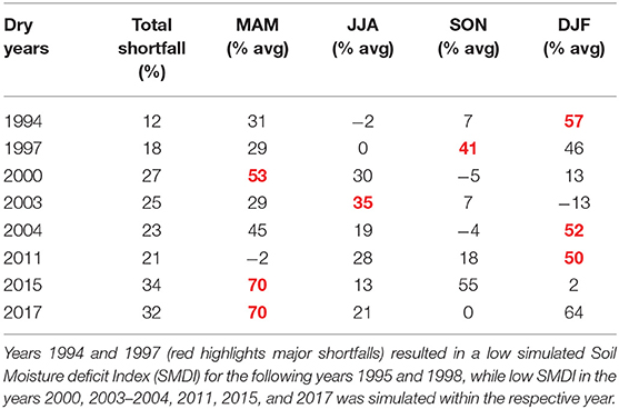
Table 1. The difference in precipitation of a three-month split of the long-term average for the years (– value shows increase, + values decrease) 1994, 1997, 2000, 2003–2004, 2011, 2015, and 2017 for the catchment.

FIGURE 3

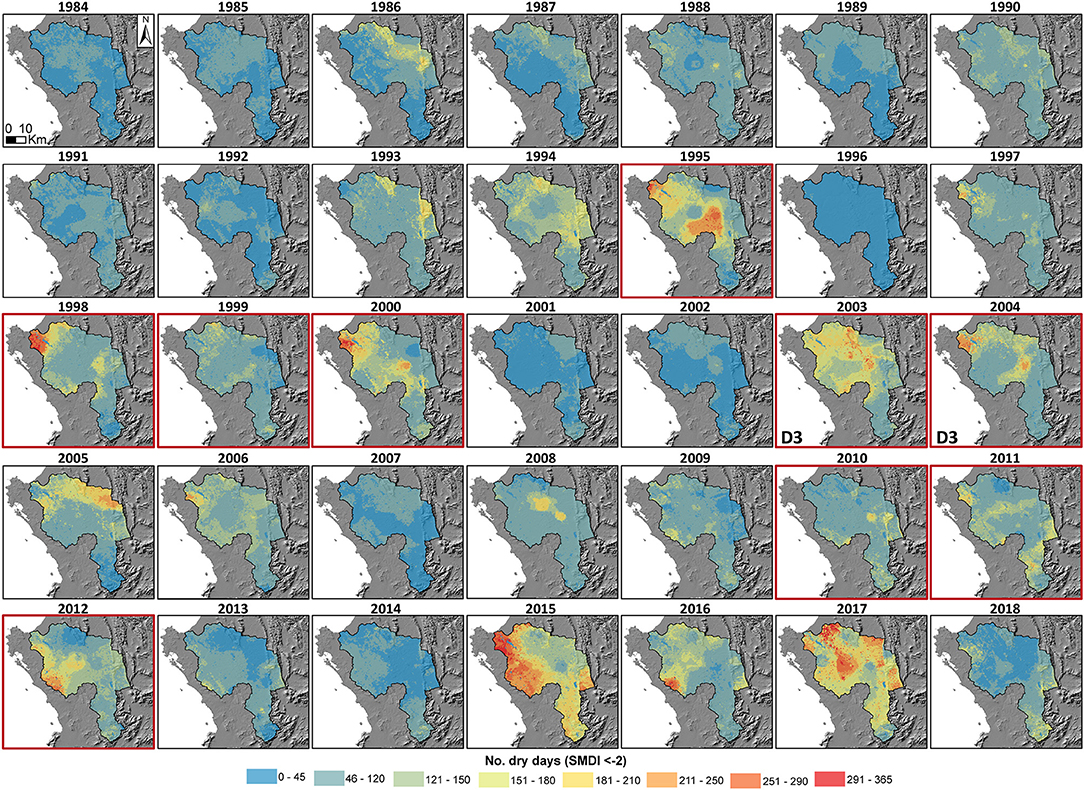
Figure 3. The number of dry days where the simulated Soil Moisture Deficit Index (SMDI) was between −2 and−4 for the periods 1984–2018 for the Berg River catchment. Severely dry years included: 1995, 2000, and 2003/2004, where >250 dry days were simulated for parts of the catchment. The droughts of 1995, 2000, and 2012 were influenced by prior dry years (>120 dry days). Unlike these droughts, 2003/2004 and 2015/2017 were preceded by wet years. While similarities between the onset of the 2003/2004 drought, the 2015/2017 drought was significantly drier and possibly influenced by anthropogenic water use (after Watson et al., 2022). Source: https://www.elsevier.com/about/policies/copyright.

TABLE 2

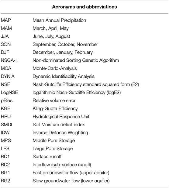
Table 2. A list of the commonly used acronyms and abbreviations used for this study.

Materials and Methods

The Berg River was modeled using the JAMS/J2000 distributed rainfall-runoff model (Krause, 2001, 2002; Krause and Kralisch, 2005) which was used to simulate the catchment hydrological processes (Figure 1). These include the model's ability to conceptually simulate processes which result in the generation of surface runoff, interflow (sub-surface runoff) and baseflow, as well as flow dynamics at a hillslope/small scale (Figure 4). The model was run on a daily timestep for the periods 1983–2018 with a 1-year initialization period (1983). The spatial modeling units were determined by following a Hydrological Response Unit (HRU) delineation procedure after Flügel (1995), together with a river reach delineation after Pfennig et al. (2009). Together with a minimum sub-basin size (7.2 km²), HRU size (0.4 km²) and a map overlay procedure the web-based GRASS-HRU delineation tool (Schwartze, 2008) was used to create the model HRUs and reach segments. The climate forcings were determined through a model regionalization approach, using local input data. Below a description is provided of the model input data, the model calibration/validation, the streamflow time of concentration and the sensitivity analysis. The methodological approach focused on the modifications made between the long-term, “dry” and “wet” period calibrations, as well as the analysis using DYNIA for temporal model uncertainty. For further details regarding the HRU delineation, the regionalization procedure of the climate data and model based calculations refer to Watson et al. (2020) and Krause (2001). Furthermore, only a summary of the model input data was presented, as a detailed breakdown of the model input data is available in Watson et al. (2020, 2021a, 2022).

FIGURE 4

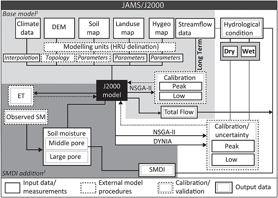
Figure 4. A schematic of the process-oriented JAMS/J2000 distributed rainfall-runoff model (after Krause, 2002), the input data, Hydrological Response Unit Delineation (HRU) and variables required for the base model (after Watson et al., 2020), the addition of the Soil Moisture Deficit Index (SMDI) component (after Watson et al., 2022) used for the assessment of “wet” and “dry” years. The use of the NSGA-II (Non-dominated Sorting Genetic Algorithm: Deb et al., 2002) to refine parameters for “wet” and “dry” years which form the upper and lower bounds (θ_dry; θ_wet) used in the Dynamic Identifiability Analysis (DYNIA: Wagener et al., 2002).

Model Inputs

The input data for the JAMS/J2000 model include spatial and temporal data. The climate forcings (including all climate variables) and streamflow measurements form the temporal data for the model, while a Digital Elevation Model (DEM) and maps of hydrogeology, soil and land use form the spatial data used in the HRU delineation. The climate forcings were collected from the World Meteorological Organization (WMO) as Global Surface Summary of the Day (GSOD) data (NOA, 2016), the Agricultural Research Council (ARC), the South African Weather Services (SAWS) and the Department of Water Affairs and Sanitation (DWS). The gap filled SRTM 90 m (Shuttle Radar Topography Mission), was the DEM which was used. A 1:250,000 geological map (Visser and Theron, 1973; Theron, 1990; CGS: Gresse, 1997), the Harmonized World Soil Database (HWSD) (Version 1.2) (Batjes et al., 2012) and the 2013–2014 South African National Land-Cover dataset (GeoTerraImage, 2015) formed the maps of hydrogeology, soil and land use which were used. Additionally, regional literature and pedotransfer functions (Schaap, 2002) were used to parameterize the spatial data for the model.

Climate Forcings and Streamflow Data

Daily totals of precipitation, solar radiation, as well as daily average windspeed, relative humidity and air temperature were collected for the periods 1983-11-01 to 2018-12-31 (±35 years). Additionally, daily minimum and maximum air temperature were required for the calculation of potential evapotranspiration rate using calculations by Allen et al. (1998). The total number of stations were 49 for precipitation, 16 for air temperature, 11 for relative humidity, 14 for windspeed and six for solar radiation. Of these stations, not all records covered the 35-year simulation, which was important for the selection of the regionalization approach. Although Kriging and other geostatistical approaches result in a lower measurement bias (Borga and Vizzaccaro, 1997), Inverse Distance Weighting (IDW) was used as it performs well for dense station networks (Dirks et al., 1998), as well as being more robust in terms of missing records (Ly et al., 2013; Watson et al., 2020). To understand the relative HRU to precipitation station distance which impacts model temporal uncertainty, a separate modeling approach which computes the regionalization statistics for each HRU, as well as a spatial aggregate for the entire model run was used (Watson et al., 2020).

Daily average streamflow was available from 27 gauging locations across the catchment. Although, of these gauges, 19 had poor record quality and were impacted by upstream reservoirs. While a multi-gauged calibration could be used to constrain differences in sub-basin hydrological processes for the Berg River, the bulk signal from the most downstream gauge was used in this study. Records from the most downstream, relatively natural G1H013 (Drieheuwels) 1983-11-01 to 2018-12-31 were used as the bulk of the catchment river flow (Figure 2). Additional reservoir outflow from the Berg River dam (G1H077 gauge) and Wemmershoek dam (G1H080 gauge) for the periods 2006-06-01 to 2018-10-01 were included in the model. To account for reservoir operations, the outflow from each reservoir was included by substituting the observed data with the simulated streamflow for reservoir reach segments for time periods where reservoir release data was available. For further detail and a description on the simulation of reservoir outflow using the JAMS/J2000 refer to Watson et al. (2022).

Spatial Parameters

Local hydrogeological literature (Conrad et al., 2004; SRK, 2009), bulk aquifer properties (Domenico and Schwartz, 1990; Tankard et al., 2012) and previous JAMS/J2000 models for the region (Bugan, 2014; Treumer, 2016; Watson et al., 2018, 2019, 2020, 2021a,b, 2022) were used to determine: (1) maximum storage capacity, (2) storage coefficient, (3) maximum aquifer thickness, and (4) recession coefficient of the upper and lower aquifer. The upper (primary) aquifer is a conceptual representation of quaternary sediments, weathered material and fractured rock aquifers and is indicative of fast groundwater within the JAMS/J2000 model. The lower (secondary) aquifer represents the regional groundwater contribution of shales and the basement aquifer, as slow groundwater in JAMS/J2000.

The Rosetta lite pedotransfer function (Schaap, 2002) within the HYDRUS model (Šimunek et al., 2006), together with the HWSD textural characteristics [% Sand, Silt and Clay (SSC)] were used to determine the input soil parameters for the JAMS/J2000 model. The model makes use of two soil pore storages namely; Middle Pore Storage (MPS: 0.2–50 μm) and Large Pore Storage (LPS: >50 μm). The soil textural characteristics were used to generate soil hydraulic properties (theta vs. depth), using a constant upper and lower head boundary, for 0, 60, and 15,000 mbar pressure ranges. The available water holding capacity (AWC) of the soil, represented as MPS, was determined by subtracting the soil water holding at 15,000 and 60 mbar. LPS was determined by the subtraction of the water holding capacities at 0 and 60 mbar. The effective water holding capacity of these soil water storages were determined by multiplying the derived water holding capacities by the effective soil depth from HWSD. Two calibration parameters, AC adaption (LPS) and FC adaption (MPS) were additionally used to scale the air capacity and AWC of the soil according to the simulated streamflow.

The land use parameters: (1) albedo (%), (2) monthly surface resistances assuming sufficient water supply, (3) Leaf Area Index (LAI) for vegetational growth periods, (4) effective vegetation heights for growth periods, (5) root depth, and (6) sealed grade value (impervious areas) are required by the JAMS/J2000 model. Local and international literature (Johnson, 1983; Van, 1984; Crain, 1998; Amer and Hatfield, 2004; Munitz et al., 2017) were used to determine the land use parameters for the respective map land use classes. Additionally, vegetation interception (a_rain) and linear reduction of potential evapotranspiration (soilLinRed) calibration factors were used to scale evapotranspiration and interception according to the simulated streamflow.

Model Calibration and Validation

In general, conceptual rainfall-runoff models can be written after Wagener et al. (2002) as:

\begin{array}{l} (ŷ t | θ) = g (t | I, θ) & (1) \end{array}

where I is a matrix system input, t is the timestep, θ is a parameter vector or parameter set, g(.) is a collection of usually non-linear functions and ŷ is the simulated system output at timestep t using parameter set θ. The objective of the automated calibration procedure, the Non-dominated Sorting Genetic Algorithm NSGA-II (Deb et al., 2002), was to estimate θ that best represents the conditions of the natural system using pre-defined parameter vector thresholds (θ_max|θ_min). The evaluation of θ is performed as:

\begin{array}{l} ε (t | θ) = y (t) - ŷ (t | θ) & (2) \end{array}

where y (t) is the observed system output. The residual, which represents the objective function (OF) and used to assess model performance efficiency, made use of different criteria to assess aspects of the simulated hydrograph (Legates and McCabe, 1999; Moriasi et al., 2007; Kundzewicz et al., 2018). The selected efficiency criteria used by the NSGA-II included the Nash-Sutcliffe Efficiency (NSE; Nash, 1970) in standard squared form (E2), logarithmic form (logE2), with the relative volume error (pBias) and the Kling-Gupta-Efficiency (KGE; Gupta et al., 2009) used as post-hoc performance evaluation outside the optimization process. The calibration procedure was applied three times, 10,000 model runs each, optimizing the objective function for the different periods: 1984–1995 as a long-term series, 1995, 1998, 2000, 2003–2004, and 2011 as dry periods only and 1984–1997, 1999, 2001–2002, and 2005–2010 as wet periods only (after Watson et al., 2022). These calibrations resulted in the determination of θ_long−term; θ_dry and θ_wet which best represent the natural system during the selected periods. A subsequent validation using θ_long−term was performed for the periods 1996–2004, 2009–2014, and 2015–2018 using θ_dry. The validation included assessing the model's performance prior and post the Berg River reservoir construction and where release data was not measured (from either of the reservoirs: 1996–2004) and where reservoir release data was available (2009–2014). The validation of θ_dry.parameter set was evaluated in terms of the most recent drought (2015–2018). Given that there were limited high altitude available precipitation stations, the modeling approach was not tailored to simulating flood extremes, as future more frequent droughts are the most concern for the WC. As a result, the evaluation of θ_wet was done using the entire “wet” timeseries (calibration only) to contrast the parameters for θ_long−term and θ_dry.

Streamflow Time of Concentration

The rate at which simulated streamflow reaches the catchment outlet using the different parameter sets (θ_long−term, θ_dry, and θ_wet) was determined through a theoretical model procedure. This involved modifying the input precipitation data, selecting a long model initialization period with no precipitation events and removing the reservoir outflow components from the model. A timeseries which includes one large precipitation event (100 mm/day on 01-01-1985, zero values for the other timesteps) for a single station/interpolation position was used as the input precipitation data. To ensure that the peak flow rate could be easily detected, a long model initialization was used (2 years-01-01-1983) to allow the storages to stabilize. The streamflow time of concentration was then calculated as the difference between the time of the one event and the flow rate peak at the catchment outlet.

Sensitivity Analysis

The Monte-Carlo-Analysis (MCA), together with the Dynamic Identifiability Analysis (DYNIA: Wagener et al., 2002) was used to understand the relative importance/uncertainty of the different parameters in the simulated hydrological processes of the Berg River using the J2000/JAMS model. The approach utilized 5000 model runs with the Nash-Sutcliffe Efficiency (NSE; Nash, 1970) in standard squared form (E2) and logarithmic form (logE2) as evaluation criteria. In order to understand the relative sensitivities of the parameters θ and ones influenced by climatic disturbances, θ_dry values were compared with θ_wet from the NSGA-II calibration. To reduce the overall number of parameters and to include parameters with the most notable solution direction differences, parameters identified as the most sensitive in a previous study were selected for the MCA and DYNIA (Watson et al., 2021b). These parameters likewise were presumed to have the largest impact (most sensitive) on the simulated streamflow time of concentration. Using a met-model approach the MCA parameters were increased/decreased between θ_dry and θ_wet. Furthermore, the effects of these increases/decreases on the simulated streamflow were determined. The results from the MCA were analyzed using DYNIA for the periods 1984–2014 with a moving window of 300 days and a fixed box count of 10 with an interval of 100.

Results

To understand the factors which impact model performance during periods of drought, these results included the simulated and observed streamflow during dry periods (1995, 1998, 2000, 2003–2004, and 2011) using parameter sets θ_long−term and θ_dry. Additionally, parameters set θ_long−term and θ_wet were used as a comparison for wet (1984–1997, 1999, 2001–2002, and 2005–2010) periods. The different parameter sets were used to understand conceptual rainfall-runoff relationship changes which occur during these periods and how the model parameter adjustments were required to capture this behavior. The analysis of these different parameter sets included the breakdown of the water balance, with particular reference to the storage changes. The temporal uncertainty analysis (DYNIA), together with the SMDI simulation of the catchment (after Watson et al., 2022) were used to identify parameters affected by “dry” and “wet” periods. Surface runoff as RD1, interflow as RD2, fast groundwater flow as RG1 and slow groundwater flow as RG2 represent the conceptual simulated flow components by the model. Likewise, they are visualized using the hydrographs but also spatially as a sub-catchment flow contribution in the results. For further region-specific drought characterization refer to Section ENVIRONMENTAL SETTING (Watson et al., 2020, 2022).

Simulated and Observed Streamflow

While the JAMS/J2000 model was run on a daily timestep and performance evaluated using daily data, the resultant plots and tables aggregate streamflow as daily averages each month, and as an average three-month yearly split (DJF, MAM, JJA, SON) to depict the model's ability to simulate the seasonal dynamics of the catchment. In general, and using the long-term parameters, the model was able to achieve a E2 of 0.59, LogE2 of 0.50 and bias of 0.15 for the dry periods compared with the long term (1984–1995) calibration with an E2 of 0.81, LogE2 of 0.87 and bias of −0.07 (Table 3, Figure 5). The long-term parameters generally underestimated streamflow during DJF months by 38% with an average simulated streamflow of 1.7 m³s⁻¹ for January months compared with the observed of 3.0 m³s⁻¹ (Figure 5). MAM and SON months were better simulated with an average difference of 10%, most noticeably with an average simulated streamflow of 7.3 m³s⁻¹ compared with the observed of 7.3 m³s⁻¹ for the October months. Unlike the model under simulations for DJF, MAM and SON months, the model tended to over simulate streamflow in JJA by as much as 29%, highlighted by an average simulated streamflow of 31.1 m³s⁻¹ compared with the observed of 21.8 m³s⁻¹. The 1996–2004 model validation using the long-term parameters achieved a E2 of 0.77, LogE2 of 0.70 and bias of −0.01 compared with a E2 of 0.80, LogE2 of 0.82 and bias of 0.02 for the periods 2009–2014 (Watson et al., 2022).

TABLE 3

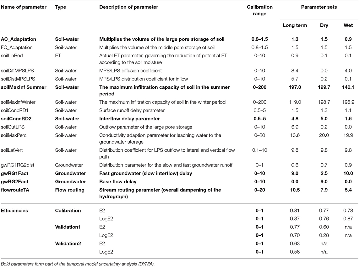
Table 3. The selected parameters (from the NSGA-II) used for the JAMS/J2000 model to capture the hydrological behavior of the Berg River catchment, showing the Nash-Sutcliffe Efficiency (NSE; Nash, 1970) in standard form (E2), logarithmic form (logE2) results for the calibration (long-term 1984–1995, dry 1995, 1998, 2000, 2003–2004, and 2011, and wet 1983–1997, 1999, 2001–2002, and 2005–2010) and validation periods (1: long-term 1996–2004, 1: dry 2015–2018) (2: long-term 2009–2014).

FIGURE 5

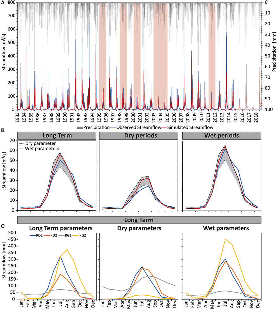
Figure 5. (A) The long-term (1984–2018) time series of the simulated (red line) and observed streamflow (blue line) with precipitation (gray bar) and the identified dry periods (1995, 1998, 2000, 2003–2004, and 2011) (pink bar). (B) The simulated monthly hydrograph for the long term timeseries, dry and wet periods using θ_long−term, θ_dry and θ_wet where the dry (dashed line) and wet (black line) parameters form the upper and lower simulation limits (grayed area). (C) The difference between the simulated hydrological flow components using θ_long−term, θ_dry and θ_wet where RD1 was surface runoff (blue line), RD2 was interflow (orange line), RG1 was fast groundwater flow (gray line) and RG2 was slow groundwater flow (yellow line). θ_long−term and θ_wet had a similar flow component breakdown with a dominance of surface runoff and slow groundwater flow, unlike θ_dry where the flow components were more equally split between surface runoff and interflow with fast groundwater the next most dominant.

Using the dry parameters, the model calibration was able to achieve a E2 of 0.77, LogE2 of 0.76 and bias of 0.03 for the dry periods (Figure 5B). The dry parameters generally overestimated streamflow by 5% for DJF and JJA months, while streamflow for MAM months were overestimated by as much as 13%. The best simulated streamflow was for February months with 3.0 m³s⁻¹ compared with an observed of 3.0 m³s⁻¹. The worst months include May with a simulated streamflow of 11.0 m³s⁻¹ compared with 8.4 m³s⁻¹ which was observed. Unlike the model overestimations for DJF, JJA, and MAM months, SON was underestimated by around 9% with most noticeable deviations for September months with a simulated streamflow of 11.7 m³s⁻¹ compared with 14.5 m³s⁻¹ observed. For the validation period the “dry” parameters achieved an E2 of 0.60, while LogE2 was 0.28.

For the wet periods, the model calibration achieved a E2 of 0.74, LogE2 of 0.82 and bias of 0.01 using the wet parameters (Figure 5B). In comparison, the long-term parameters resulted in a E2, LogE2 and bias of 0.70, 0.78, and −0.04, respectively, for the wet periods. In general, the wet parameters underestimated streamflow in DJF and SON by as much as 27%, highlighted by an average simulated streamflow of 6.0 m³s⁻¹ compared with an observed of 8.2 m³s⁻¹ for November months. MAM and JJA streamflow tended to be over simulated by as much as 18% and in particular for June where daily average simulated streamflow was 55.7 m³s⁻¹ compared with 44.7 m³s⁻¹ observed.

Simulated Flow Components

While the hydrographs were used to compare the long-term, dry and wet parameters for the entire modeling duration (1984–2014), the spatial plots and contribution statistics (Table 4) compare the dry and wet parameters with long term parameters under both dry (Figure 6) and wet (Figure 7) periods.

TABLE 4

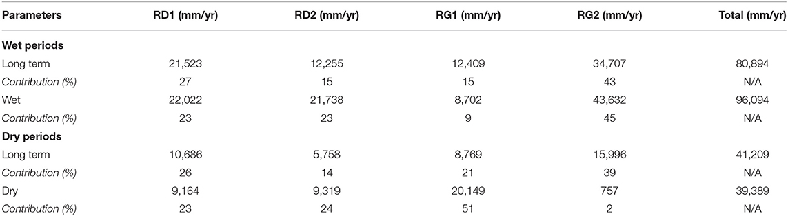
Table 4. A summary of the total flow contribution and the percentage of simulated surface runoff (RD1), interflow (RD2), fast groundwater (RG1) and slow groundwater (RG2) using the parameters θ_long−term, θ_wet and θ_dry for wet periods (1983–1997, 1999, 2001–2002, and 2005–2010) and dry periods (1995, 1998, 2000, 2003–2004, and 2011).

FIGURE 6

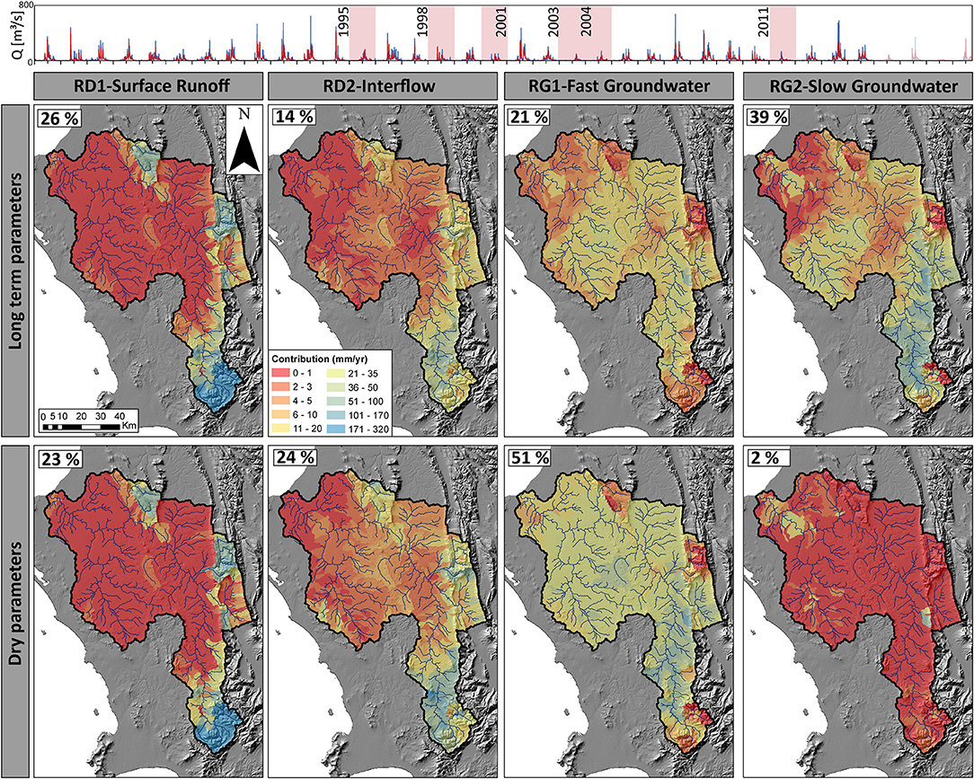
Figure 6. The long-term (1984–2018) time series of the simulated (red line) and observed streamflow (blue line) with the yearly contribution of surface runoff (RD1), interflow (RD2), fast groundwater (RG1) and slow groundwater (RG2) for the identified dry periods (1995, 1998, 2000, 2003–2004, and 2011) using the parameters θ_long−term and θ_dry with the average percentage contribution for each of the flow components. Spatially θ_long−term and θ_dry were similar, with a dominance of flow in the catchment headwater areas (south), but differed by the total contribution for interflow (10%), slow (30%) and fast groundwater (37%).

FIGURE 7

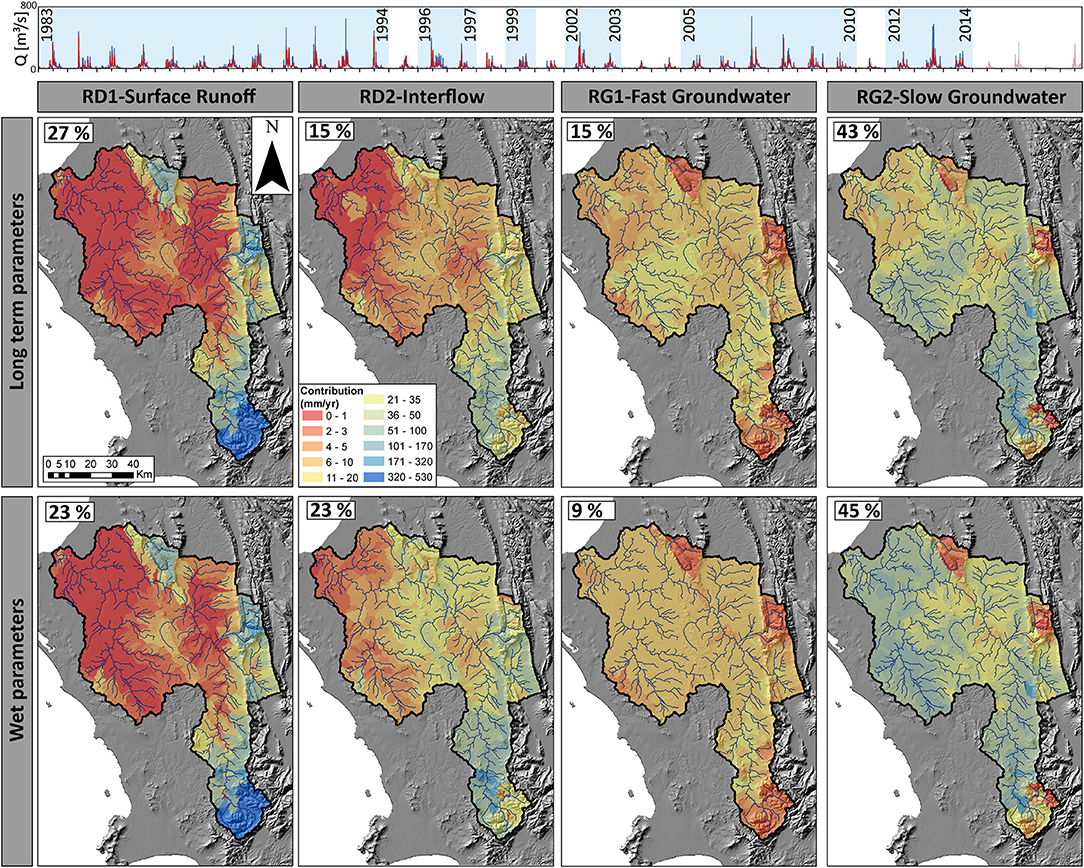
Figure 7. The long-term (1984–2018) time series of the simulated (red line) and observed streamflow (blue line) with the yearly contribution of surface runoff (RD1), interflow (RD2), fast groundwater (RG1) and slow groundwater (RG2) for the identified wet periods (1983–1997, 1999, 2001–2002, and 2005–2010) using the parameters θ_long−term and θ_wet with the average percentage contribution for each of the flow components. Spatially θ_long−term and θ_wet are similar, but differ by the contribution of interflow (8%) and fast groundwater (6%).

The hydrograph of the long-term parameter model was dominated by RG2 with 40% of the total flow, followed by RD1, RG1, and RD2 with 27, 17, and 16%, respectively (Figure 5C). August generated the largest amount of RG2 with 375 mm/year followed by 323 mm/year of surface runoff in July. The hydrograph of the wet parameter model was likewise dominated by RG2 but with 42% of the total flow, followed by RD2, RD1, and RG1 with 24, 22, and 12%, respectively. July generated the largest amount of RG2 with 454 mm/year followed by 414 mm/year for RG2 in August. The hydrograph of the dry parameter model was likewise dominated by groundwater, but in the form of RG1 with 43% of the total flow, followed by RD2, RD1, and RG2 with 28, 24, and 5%, respectively. July generated the largest amount of flow, but in the form of RD1 with 245 mm/year followed by 235 mm/year for the same month from RD2.

During the dry period, RD1 using both the long-term and dry parameters was dominated by contributions from the catchment headwaters (southern tip and east boundary) with only a 3% contribution difference between the two parameter sets and a flow of 170–320 mm/yr (Figure 6). While there was a 10% contribution difference in RD2 between the long-term and dry parameters, similar spatial contributions were simulated for the dry period. Using the long-term parameters groundwater flow was split between RG1 and RG2 as 21 and 39%, respectively for the dry period. RG2 using the long-term parameters simulated major contributions from valley areas in the south and east boundary of the catchment. Unlike the groundwater contribution using the long-term parameters for the dry period, when using the dry parameters RG1 contributed 51% compared with only 2% from RG2. Furthermore, the catchment valley contributed limited RG2 and the bulk from RG1 of 20–100 mm/yr for most of the valley sub-catchments.

During the wet period, RD1 was simulated as a maximum of 530 mm/yr in the catchment headwater area (Figure 7) with a parameter set contribution difference of 4%. The parameter sets produced similar representations of RG1 and RG2, differing by 6 and 2%, respectively. Spatially valley areas contributed the most RG2 with between 35 and 100 mm/yr for both the long-term and wet parameter sets. RD2 was the major difference in the simulated flow components between the long-term and wet parameter sets with an 8% difference and between 2 and 20 mm/yr flow nearest the outlet compared with 0–5 mm/yr flow for the long-term parameters.

Simulated Water Balances and Time of Concentration

Overall, simulated streamflow as a percentage of the total water balance (including storage changes) was simulated as 15, 13, and 16%, respectively for the long-term, dry and wet parameter sets for the periods 1984–2014 (Figure 8). Simulated storage, which was determined as the difference between precipitation, evapotranspiration and streamflow, was between −177 (loss) and 79 (gain) mm/yr for the wet parameter set, compared with −43 to 23 mm/yr and −37 to 20 mm/yr for the long-term and dry parameter set, respectively. For the dry years 1995 and 1998, both long-term and dry parameter sets simulated a storage gain, with an average of 13 and 11 mm/yr respectfully. The dry years 2000, 2003–2004, and 2011 were simulated as a storage loss, with an average of −4 and −2 mm/yr using the long-term and dry parameter sets. Wet years, such as 1996, 2001, and 2002 were simulated with an storage loss of 117 mm/yr using the wet parameters compared with 2 mm/yr for the long-term parameters. The resultant effect of the dry, wet and long-term parameters was a streamflow time of concentration (TC) of 4, 2, and 5 days, respectively.

FIGURE 8

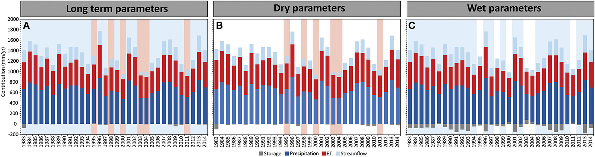
Figure 8. The simulated water balance (mm/yr) for the periods 1984–2014 (including 1 year of initialization 1983 to show storage stabilization), which includes yearly precipitation (P: blue bar), evapotranspiration (ET: red bar), streamflow (Q: light blue bar) and storage (ΔS: gray bar) using the (A) θ_long−term, (B) θ_dry, and (C) θ_wet parameter sets. (B) θ_long−term and θ_wet differ with simulated storage (55 mm/yr), but was similar in terms of ET (12 mm/yr). θ_long−term and θ_dry were similar in terms of simulated storage (1 mm/yr) but differ in terms of simulated ET (27 mm/yr).

Temporal Model Uncertainty

The deviation between the upper and lower bounds for the simulation period (1984–2014) and changes in the “best” parameter value (dark gray pixels) illustrate parameters which impact the temporal uncertainty of the model (Figure 9). The impact of the baseflow delay parameter (gwRG2Fact) and the maximum infiltration capacity of the soil (soilMaxInfSummer) was limited, as the “best” value for gwRG2Fact was constant at <0.02 and 155 for the soilMaxInfSummer parameter (but had limited sensitivity). During the periods 1995–2005, the surface runoff delay parameter (soilConcRD2) was stable and “best” around the maximum value of 4.8. For the same period, scaling of air capacity (AC_Adaptation) had likewise limited temporal uncertainty with a “best” value of 1.45, but uncertainty increased during the transition between wet and dry periods (Figure 10). The fast groundwater delay parameter (gwRG1Fact) during the periods 1995–2005 was temporally uncertain during the transition between dry and wet periods, but mostly tended toward a “best” value of 3. The streamflow routing parameter which dampens the overall hydrograph (flowrouteTA) for the periods 1995–2005 tended around the “best” value of 7.8, but was more optimal at 5.5 during the wet periods between 2001 and 2003 (Figure 9). For the periods 1984–1994 and 2005–2010, which were mainly wet, AC_Adaptation, gwRG1Fact and SoilConcRD2 the optimal values varied between the upper and lower bounds. The drought of 2011 resulted in temporal uncertainty in AC_Adaptation, gwRG1Fact, SoilConcRD2 and wet periods of 2012–2014 resulted in the “best” value of flowrouteTA tending to 5.5 compared with prior values of 7.8.

FIGURE 9

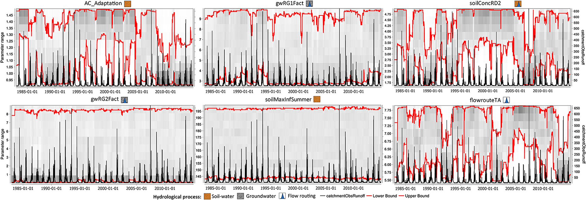
Figure 9. The Dynamic Identifiability Analysis (DYNIA: Wagener et al., 2002) using the Nash–Sutcliffe (NSE; Nash, 1970) efficiency in standard form (E2) for the selected parameters showing the upper and lower parameter bounds of the Monte Carlo Analysis (MCA: red line). The soil-water parameters include scaling of air capacity (AC_Adaption), the Surface runoff delay parameter (SoilConcRD1) and the Maximum infiltration rate during summer parameter (soilMaxInfSummer). Groundwater parameters include Fast groundwater delay (gwRG1Fact), Slow groundwater delay (gwRG2Fact). The routing parameters include the Surface runoff delay parameter (SoilConcRD1), Fast groundwater delay (gwRG1Fact), Slow groundwater delay (gwRG2Fact) and the stream routing parameter (FlowrouteTA). Parameters which have temporal uncertainty show a variability in the upper and lower parameter bounds and where the “best” parameter sets (gray blocks) varies across the simulated time series. These parameters include the AC_Adaption, gwRG1Fact, SoilConcRD1 and FlowrouteTA.

FIGURE 10

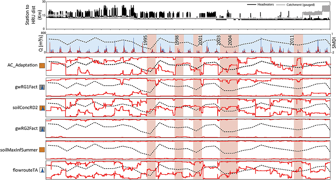
Figure 10. The precipitation to HRU distance in the catchment headwater (black line) and for the gauged portion (gray line), simulated (red line) and observed streamflow (blue line), the simulated Soil Moisture Deficit Index (black dashed line) (after Watson et al., 2022). The upper and lower bounds of the Dynamic Identifiability Analysis (DYNIA) using the Nash–Sutcliffe (NSE; Nash, 1970) efficiency in standard form (E2) for the selected parameters showing temporal parameter uncertainty, considering the station to HRU distance, simulated SMDI and the streamflow for different “dry” and “wet” periods. The alignment of these three datasets show three periods of similar model uncertainty from 1984–1994, 1995–2005, and 2006–2014.

Discussion

The application of conceptual rainfall-runoff models calibrated under relatively common normal, i.e., well understood, climatic conditions can significantly affect the interpretation of hydrological responses both observed under climate extreme conditions, and their projection using future climate scenarios. Such application risks the advancement of mal-adaptive responses to climate change, and inappropriate allocation of scarce resources. Given the risk that climate change poses to the Western Cape and much of semi-arid Southern Africa, the aim of this paper was to assess model related performance and uncertainty under extreme climate conditions, referred to as “wet” and “dry” periods and the applicability of conceptual rainfall-runoff models for future climate change-based assessments in Africa. Natural vegetation cover changes in the Berg River were estimated to have increased by more than 14% from 1986/7 to 2007 (Stuckenberg et al., 2012), which impacts streamflow and temporal model uncertainty, but were not considered. Furthermore, irrigation which was estimated as 5% of the total catchment area (van Niekerk et al., 2018) did not form part of the modeling approach, due to limitations in the current water use estimates for different vegetation types in the catchment.

A shift by the agricultural sector and the increase in domestic groundwater use has been suggested to aggravate the drought conditions in the Western Cape of South Africa and the meteorological and agricultural droughts progression to more severe long-term forms (hydrological and groundwater drought) (Watson et al., 2022). This was supported by local aquifer level measurements, satellite-based groundwater thickness reductions (Gravity Recovery and Climate Experiment: GRACE) and hydrological change drawn from rainfall-runoff models. While, the presumed increase in groundwater use was supported by a multitude of factors, current rainfall-runoff models assume stable storage conditions and the signal to noise ratio (Xue et al., 2013) during dry periods affects model performance and uncertainty. This approach uses the JAMS/J2000 model as a metric of other conceptual rainfall-runoff models, but large differences in the representation of hydrological processes have even been reported between different conceptual rainfall-runoff models where the signal to noise ratio is low (Arnaud et al., 2011; Hattermann et al., 2017; Eeckman et al., 2019). Furthermore, it is likely that more physically based models, such as SWAT (Arnold et al., 1998) and TOKAPI (Ciarapica and Todini, 2002) could respond differently to climatic extremes based on model structures, but also when considering additional measures of hydrological processes (soil moisture, evapotranspiration, deep percolation) to validate process simulations.

Impact of Climate Extremes on Model Uncertainty

In a related study for the Berg River, Watson et al. (2022) illustrated that the performance of the JAMS/J2000 model varied for different “dry” and “wet” years and where a “good” simulation (NSE > 0.6: Waters, 2014), using a single long term parameter set, was possible for a yearly meteorological shortfall of 28%, which also corresponded to a 53% reduction in MAM precipitation. After this threshold was exceeded, model related performance dropped to an NSE of 0.59 in 2000, and more significantly to 0.26 (Watson et al., 2022) for the years 2015–2017 (although groundwater abstractions were not considered by the model), where the meteorological shortfall was 32–34% (70% reduction in MAM precipitation). As dry periods lower the signal to noise ratio and the water balance becomes tighter, different parameter combinations become better suited and changes in simulated flow components can often be required. Furthermore, seasonal shift such as the reduction of precipitation for MAM, which reduces soil-moisture prior to winter (JJA), impacts streamflow dynamics and peak flow. Most noticeable were changes to the time of concentration, where TC reduced by 1 day between the different dry and long-term parameters. Furthermore, there were changes to the overall contribution of fast and slow groundwater, but these flow components are more conceptual than driven by physical data. The overall outcome on the simulated hydrology using the long-term, “dry” and “wet” parameters is not unexpected given that this study utilizes a single downstream calibration. River flows in the Berg River catchment are particularly dependant on headwater contributions, and while these areas were highlighted as the most affected in Watson et al. (2022), the headwater gauging records show the largest amount of change and a concern for regional water security.

The temporal uncertainty analysis DYNIA showed parameter sensitivity changes during different “dry” and “wet” periods (Figures 8, 9). In particular, the scaling of air capacity (AC_adaptation), a highly sensitive parameter which can affect the simulation of different flow components and TC, showed uncertainty after 2004 and remains stationary past the drought of 2011 where SMDI was between −0.5 and 0.5. Some of this uncertainty, can be attributed to the construction of the Berg River dam in 2004 which also affected the temporal uncertainty of the simulated interflow rate (soilConcRD2) and not represented by SMDI. The use of the reservoir component, which substitutes simulated streamflow with reservoir outflow, could further affect model parameter sensitivity after 2006. While there was still a large amount of noise using DYNIA for the periods 1984–1994, where SMDI was between 0.3 and −0.5, the shift between “dry” to “wet” conditions or vice versa, resulted in the largest amount of parameter uncertainty for the analysis period. From our study we conclude that links between temporal model uncertainty and meteorological/agricultural drought indices can improve the understanding of model capabilities in the light of future non-stationary climate conditions, although data availability and its variability influences model applications in Southern Africa. Furthermore, reliable forecasting systems at seasonal and sub-seasonal scale require the integration of hydrological modeling tools with other hydro-climatic indicators and tracers to consider the associated system change during climatic instabilities.

Development of Dynamic Parameter Rainfall-Runoff Models

The number of parameters with which a model simulates hydrological behavior is an important consideration during model development. Too few parameters result in poor seasonal and sub-seasonal simulations, while too many parameters result in model overfitting (e.g., Whittaker et al., 2010). The use of a set of “dry” parameters improved the model's performance for the dry analysis period (E2 of 0.59–0.76 and LogE2 of 0.50–0.78), as well as the 2015–2018 validation period with an improvement of E2 from 0.26 to 0.60. The availability and variability of climate data impacted the predictions made after 2014 (Figure 10), where the precipitation station to HRU distance increase by 5 km (15–20 km). Anthropogenic groundwater extraction may have affected the residual between simulated and observed low flows, although logE2 improved from 0.17 to 0.28 for the periods 2015–2018 when switching from the long-term to the dry period parameters. While the use of “wet” parameters also improved model performance for the wet periods (E2 0.70–0.74 and LogE2 of 0.78–0.82), these improvements are less significant for semi-arid WC. The resultant effect is that for future predictions in Mediterranean WC, a “dry” set of parameters are recommended for periods where meteorological shortfalls exceed 28% per year and where MAM precipitation is reduced by more than 50%. As a result, a dynamic parameter model, which may use drought indices, such as the Standardized Precipitation Index (SPI) or Standardized Precipitation Evapotranspiration Index (SPEI), as triggers has the potential to better account for climate extremes. While a “wet” parameter set is not recommended in the context of semi-arid Southern Africa, it might be more applicable for tropical regions and where a shift in monsoons are expected. Although this study focuses on the use of different parameter sets for climatic extremes, it should be noted that additional effort can still be placed in selecting a single more robust parameter set. For example, the long-term and “wet” parameters have a higher groundwater contribution than the “dry” parameters and additional metrics which validate flow component proportioning could be used to refine solutions generated by the NSGA-II. Likewise, multi-site/gauged calibrations have the potential to reduce the impacts of climatic extremes on model performance. These added modeling requirements highlight the need for dynamic and flexible modeling systems, which will be required in simulating future climatic extremes and this was demonstrated by these results.

Implications for Water Management

Climate change will impact water availability and in turn likely cause changes in land use and increases in anthropogenic water use. These changes have already occurred within the 2015–2018 drought for the WC and understanding the impacts to the water cycle components and the feedback loops of different hydrological processes is important and ongoing. As groundwater becomes a resource with which municipalities and water management agencies use to reduce the risk of climate change, understanding the cause-and-effect relationship between groundwater recharge and changes in precipitation seasonality is important for the management of this resource in a sustainable manner.

Projections of future hydrological conditions, built off processed based distributed modeling, are needed by a variety of stakeholders, who oversee the management of water resources, particularly in the context of catchment water management agencies and municipalities. As the results from hydrological modeling systems become increasingly more important for water management under climate change, there is a growing need for cross sectoral management including dam management, agricultural and mining activities as well as domestic and industry water consumption for water yield planning. For assessing the impact of increasing climate extremes as anticipated in Mediterranean South Africa, this requires modeling approaches which are well-understood and verified in terms of their performance, uncertainty, limitations and potential. Additionally, the importance of continuing scientific monitoring and the development of new approaches/tools are required to reduce hydrological projection uncertainty under climatic change. In particular for the WC, understanding the increased groundwater consumption and the quantification of these amounts are required if future model predictions are to be useable.

Conclusion

The ability to simulate catchment hydrological behavior is dependent on data availability and variability, as well as the model calibration and validation approach. Predictions of hydro-meteorological extremes, such as droughts, are often not well simulated when observed infrequently within the calibration period, but crucial for the assessment of climate and hydrological risk and their current and future management. As the occurrence and duration of these extremes are likely to increase in the future in Mediterranean South Africa, model performance, uncertainty and representation need to be assessed during different climatic extremes. In our study, we have shown that a temporal uncertainty analysis provides the means to assess model parameters which are impacted by different “wet” and “dry” periods. For JAMS/J2000 model of the Berg River catchment, soil-water storage, timing of interflow, and groundwater flow, as well as the overall dampening of the simulated hydrograph were the parameters most affected by climatic extremes. Furthermore, the predicted time of streamflow concentration shifted when using different “dry” and “wet” period parameters, affecting the simulated peak flow. Although long-term model simulations are required for climate change predictions, a switch between “dry” and long-term simulations are recommended for future model applications in the region. Furthermore, long-term historical calibrations are unlikely to have the capabilities to simulate future hydrological flows and further model developments are still required for parameters affected by climate variabilities.

Data Availability Statement

The raw data supporting the conclusions of this article will be made available by the authors, without undue reservation.

Author Contributions

Conceptualization and writing—reviewing and editing: AW, PR, JH, and GM. Methodology and software: AW and SK. Data curation and writing—original draft preparation: AW and JH. Visualization and investigation: AW. Project administration: JH and GM. Software and validation: SK and AW. All authors contributed to the article and approved the submitted version.

Funding

The authors would like to thank DAAD [German Academic Exchange Service: sponsored by BMBF (The Federal Ministry of Education and Research)] and the Division for Research Development (DRD) of Stellenbosch University for funding support.

Conflict of Interest

The authors declare that the research was conducted in the absence of any commercial or financial relationships that could be construed as a potential conflict of interest.

Publisher's Note

All claims expressed in this article are solely those of the authors and do not necessarily represent those of their affiliated organizations, or those of the publisher, the editors and the reviewers. Any product that may be evaluated in this article, or claim that may be made by its manufacturer, is not guaranteed or endorsed by the publisher.

Acknowledgments

The authors would like to thank the South Africa Earth Observation Network (SAEON), Department of Water Affairs and Sanitation (DWS), South Africa Weather Service (SAWS) and Agricultural Research Council (ARC) for access to climate and streamflow records. Furthermore, the authors would like to thank three reviewers for their recommendations and comments. The publisher is fully responsible for the content.

References

Akoko, G., Le, T. H., Gomi, T., and Kato, T. (2021). A review of SWAT model application in Africa. Water 13, 1313. doi: 10.3390/w13091313

PubMed Abstract | CrossRef Full Text | Google Scholar

Allen, R. G., Pereira, L. S., Raes, D., and Smith, M. (1998). Crop Evapotranspiration—Guidelines for Computing Crop Water Requirements—FAO Irrigation and Drainage Paper 56. Rome: FAO.

Google Scholar

Allison, E. H., Perry, A. L., Badjeck, M. C., Neil Adger, W., Brown, K., Conway, D., et al. (2009). Vulnerability of national economies to the impacts of climate change on fisheries. Fish Fish. 10, 173–196. doi: 10.1111/j.1467-2979.2008.00310.x