Using a Large Climate Ensemble to Assess the Frequency and Intensity of Future Extreme Climate Events in Southern Africa

This paper uses 7,200 smoothed climate change projections for each of the four emissions scenarios, together with inter-annual variation provided by detrended historical climate data to investigate changes in growing season (wettest 3 months) weather patterns from the 2020s to the 2060s for ten countries of Southern Africa. The analysis is done in 8,888 quarter-degree pixels by month. Temperature unequivocally rises in the region, but it rises relatively less along the coasts, particularly on the eastern side of the region. Precipitation has trended downward for much of the region since 1975, but relatively little change in precipitation is projected between the 2020s and the 2060s. Under the higher emissions “Paris Forever” scenario, we found that by the 2060s, the 1-in-20-year low-rainfall events will occur twice as frequently in most of the region, though it will occur less frequently in northwestern Angola. The 1-in-20-year high-rainfall events will occur 3 to 4 times as often in northeastern South Africa and twice as often in most of Angola.

Introduction

For determining the full effect of climate change—particularly as it is applied to agriculture, but also to human life and all sectors of the economy—we must understand sources of uncertainty and sources of variability. First, there is uncertainty in regard to the future flow of greenhouse gas (GHG) emissions, and therefore in regard to future amounts of CO₂ in the upper atmosphere at points in the future. Second, even if we had full knowledge regarding the amount of CO₂, there is still uncertainty as to how the mean climate would be affected (Kunreuther et al., 2014; Chen et al., 2021; IPCC, 2021; Lee et al., 2021). Finally, even if we had certainty about CO₂ levels and mean climate, there would always be inter-annual and intra-annual variation.

In what follows, we consider four different emissions scenarios in ten countries of Southern Africa: Angola, Botswana, Eswatini, Lesotho, Malawi, Mozambique, Namibia, South Africa, Zambia, and Zimbabwe. For each of the emission scenarios, we consider 7,200 smoothed climate change projections with monthly values spanning 2019 to 2069. We also augment each of the smoothed climate projections with 100 different 51-year sequences randomly drawn by year with replacement from a 69-year detrended historical dataset. This gives us a total of 720,000 variation-augmented climate projections for each emissions scenario.

This article is an extension of earlier work on the impact of climate change in the region (Fant et al., 2015; Schlosser and Strzepek, 2015; Arndt et al., 2019) that used a large ensemble of climate models (based on the older AR4/CMIP3 rather than the AR5/CMIP5 used here) but which did not adequately address climate variability, without which, investigating changes in climate extremes is not possible. The novelty of this approach is in using a large ensemble of climate futures [100 times the size used in the previous work of Schlosser and Strzepek (2015)] so that the tails of the distribution are more fully modeled, more completely taking into account uncertainty and variability.

Collins et al. (2013) explore the range of climate model predictions from CMIP5 across various emissions scenarios and climate models at the global level, and IPCC (2013) shows maps focusing on Southern Africa. Seneviratne et al. (2012) provides a very thorough discussion on both observed and modeled weather extremes (though with a greater focus on observed), though at the global level. Seneviratne et al. (2021) updates the earlier work in the just-released IPCC assessment report.

Assessing the magnitude of climate change and the added effects of climate uncertainty and inter-annual variability enables research to better investigate the impact of climate shocks on sectors of the economy dependent on weather, such as agriculture, infrastructure, energy, and construction. In a related paper, we use the future variation-augmented climate projections to assess the impact on agricultural production in the region (Thomas et al., 2022).

Southern Africa is an important region to study the effects of climate because of the importance of agriculture to the region for its contribution to GDP, for employment, and for food insecurity, which is a problem for the region (Thome et al., 2018; FAO et al., 2020).

Materials and Methods

MIT-IGSM Future Climate Data

In this paper, we use results from a large ensemble of projected changes in monthly precipitation and near-surface air temperature for ten nations of Southern Africa (Schlosser et al., 2020, 2021). The ensemble is developed by integrating pattern-change responses derived from the Coupled Model Intercomparison Project Phase 5 (CMIP5) climate models with the Massachusetts Institute of Technology Integrated Global Systems Model (MIT-IGSM), an earth-system model coupled to a global economic model that evaluates uncertainty in socio-economic growth, anthropogenic emissions, and global environmental response.

The methodology used to combine the two relies on pattern-kernels of regional change from climate models (Schlosser et al., 2012) and the application of these patterns of change to downscale the zonal output of the MIT Integrated Global System Model (Reilly et al., 2018). IGSM operates in the dimensions of latitude and elevation (depth) only, so that they might consider a wider-range of potential climates that can develop out of assumptions surrounding emissions, demographics, and the economy. Approaches that consider the longitude with elevation and latitude take much longer to run and require much greater computing power.

In order to expand these results longitudinally, the authors use a Taylor series expansion that allows them to construct a full grid of climate-change pattern kernels, using CMIP5 climate models. There are many CMIP5 models available for use, but many centers producing these models produce more than one. The authors chose to use only one model per center to avoid biasing the ensemble's representativeness.

The MIT-IGSM produces 400 unique results for each emissions scenario. Each of these are spread out longitudinally using 18 GCMs from CMIP5 [these are detailed in Schlosser et al. (2021)], giving the ensemble 7,200 members of a hybrid frequency distribution (HFD) per emissions scenario. The version of the data used in the analysis in this paper is one in which each member is smoothed by averaging over a multi-year period, preserving the trend, or signal but removing the variation.

The MIT-IGSM evaluated four scenarios of future climate and socio-economic development to span a range of possible actions to reduce greenhouse gas emissions through the twenty-first century (Schlosser et al., 2021). These emissions scenarios are:

▪ Reference (REF): No explicit climate mitigation policies anywhere in the world. It can be seen as a baseline.

▪ Paris Forever (PF): Assumes that countries meet the mitigation targets in their Nationally Determined Contributions (NDCs) and those targets are met throughout the century.

▪ 2C: Reflects an effort to limit climate change to no higher than a 2°C global average by the year 2100 through globally coordinated, smoothly rising carbon price. This scenario reflects the uncertainty of the climate response in the MIT Earth System Model (MESM, Sokolov et al., 2018) and leads to an overall probability of having 66% of the runs using this emissions scenario keeping the global average at or below 2°C.

▪ 1p5C: Similar to the 2C, but aims to limit warming to no higher than 1.5°C. The probability of achieving this target in this emissions scenario is 50%.

To simplify the exposition in this paper, we often elect to focus on the more plausible models (our subjective interpretation): the 2C and PF.

Princeton Global Forcings Historical Weather Data

While we expect quite a range of uncertainty reflected across the possible smoothed climate change projections, we also know that year-to-year variation is quite important for agriculture and many other human endeavors. To simulate inter-annual variation in a manner that is spatially and temporally consistent, we decided to base the values on historical weather provided the Princeton Global Forcings (PGF) dataset, version 3 [based on (Sheffield et al., 2006)]. This dataset provides daily weather data for a number of weather variables, including the ones relevant to this analysis: precipitation and daily minimum and maximum temperatures. The data spans the period from the beginning of 1948 to the end of 2016. It is at a quarter degree resolution, which in most places reflects rectangles with 25–30 kilometers on each edge. For most of our work we are interested in monthly data, so we aggregate the data, summing the precipitation and computing monthly values for mean daily maximum and mean daily minimum temperatures. Because the HFD data represents deviations from the climate of 1981–2000, we also used PGF to provide this baseline climate information.

Combining Smoothed Climate Change Projections and Historical Weather Variability

Belcher et al. (2005) proposed a technique for generating feasible future weathers that account for climate change which they called “morphing.” They used it for thermal simulation of buildings, but the idea can be applied to other problems, such as assessment of future agricultural production or water availability. In their version, they added the smoothed climate “delta” (with “delta” signifying a change in a variable)—that quantifies how a smoothed (or averaged) climate variable shifts between the baseline climate and the future climate—to the historical weather value to produce what they call the “design” weather and what we will call here the “variation-augmented climate change projection.” Their method has the advantage of preserving spatial relations and temporal relations (intra-annual and inter-annual). However, as used in their original idea, it gives only one sequence of future weather at each pixel.

Augmenting smoothed climates has the advantage over the original GCMs in two ways. First, the models are downscaled to a much finer spatial resolution that is required for studies on the effect of climate on agriculture, since agricultural production (and modeling) relies on location-specific weather and land characteristics, with the original GCMs at ~250-kilometer resolution and the down-scaled resolution being ~30-kilometer resolution. Second, the original GCMs would need to be run repeatedly to give enough samples to adequately account for the tails due to both uncertainty and inter-annual variation, and those are not available and take tremendous computing power to produce.

We maintain the spirit of what Belcher et al. (2005) did, but adapt it to recognize that climate change has already affected at least some of the historical sequence, which is contrary to their implicit initial assumptions. To compensate for the climate signal that is already in the historical data, we use regressions to remove the trend and keep the variation around the trend as the value that we are interested in using to produce variation using our Monte Carlo simulation procedure. The inter-annual variation and the climate delta then both get added to the baseline climate value.

Specifically, for each variable in the historical weather dataset, we took the monthly series of 69 yearly values at each pixel and regressed them on a constant, a value for year, and a value equal to 0 for years <1975 and the year minus 1975 for values greater. This gave us a piecewise linear regression over time that assumed that the effect of climate change altered the trend in 1975. It gives us one trend prior to 1975 and one trend after 1975, but the trend lines meet at the year 1975, and therefore are dependent on each other. The year 1975 was chosen because in annual global temperature graphs, there is a clear shift in rate of temperature change that took place somewhere in the 1970s. Many studies de-trend with a straight line for the entire time period, which strikes us as wrong because it fails to acknowledge any shift in the climate since the 1940s. On the other hand, over-correcting by using some kind of non-parametric method such as loess or localized polynomial would remove inter-decadal variation, which we wanted to keep in due to the nature of the smoothing for the MIT-IGSM. There is no perfect solution, but the method used in this paper seemed better than the others considered. We estimated these regressions for each variable-pixel-month and retained the residual from each year. These are the “variation deltas” – the inter-annual variation measures – which form the basis for future random draws of weather in the Monte Carlo procedure.

Mathematically, let v_{i, yr, m} be the value of a monthly weather statistic from the PGF database for pixel i, year yr, and month m, where v is monthly precipitation or mean daily maximum or minimum temperature for the month. The variable yr75 is defined as 0 if yr ≦ 1975 and yr – 1975 if yr > 1975. We estimate the following regression:

$\begin{array}{ll}{v}_{i,yr,m}=b_{0,i,m}+b_{1,i,m}yr+b_{2,i,m}yr75+{ϵ}_{i,yr,m}& (1)\end{array}$

where b_{0, i, m} is the intercept term, b_{1, i, m} is the parameter associated with yr, b_{2, i, m} is the parameter associated with yr75, and e_{i, yr, m} is the residual of the regression, which is the variation delta that we will use to in the Monte Carlo simulation.

We also adapt the morphing method further, by generating multiple sequences of feasible future sequences of climate variations. Our idea is to keep 12-month sequences for the entire study area together as a single unit, drawing randomly with replacement from the 68 or 69 12-month sequences. Our goal is to come close to attaining ideal simulated data: one which maintains spatial relations, intra-annual relations, and minimizes the degree of inter-annual correlation that is lost by artificially breaking the data into 12 consecutive month segments.

We recognize that there is correlation in precipitation in consecutive months. It is an important characteristic of the growing season that the rainfall through the season be consistent. Since the growing season in many locations spans the time from one calendar year into the next, we decided that we did not want to use the calendar year as our unit of observation to draw for random weathers in the future. Instead, we created what we call “meteorological years” that begin during the dry season. Most specifically, they begin in the middle month of the driest 3-consecutive-month period (by pixel). This allowed us to take data from 69 calendar years and convert it into 68 meteorological years that were less serially correlated than the calendar year values.

We created baseline climate variables at each pixel to which the climate changes from the HFDs could be added. We did this by summing the daily precipitation for each pixel-year-month combination and by taking the mean of the daily minimum and maximum temperatures for each pixel-year-month. After doing this, using only data from 1981 to 2000, we took averages of these pixel-year-month combinations by pixel-month.

We added the smoothed climate change deltas by year to these baseline variables. For precipitation we added the precipitation change. For both the mean daily maximum temperature and mean daily minimum temperature we added the mean daily temperature change—which was the only temperature variable provided in the HFDs. We took the 2- by 2.5-degree smoothed climate change rectangles and assumed that the shift was identical for all of the 80 quarter-degree pixels within the historical weather dataset located within the larger rectangle. The result was quarter-degree resolution smoothed climate projections.

On top of these smoothed values, we added the variation deltas to give us variation-augmented climate projections. For each emissions scenario, we have 7,200 smoothed climate change projections, and overlaid 100 variation delta datasets on each to give us a total of 720,000 variation-augmented climate projections spanning 51 years for each month and close to 9,000 pixels.

Results

Characteristics of the Smoothed Climate Change Projections

Figure 1 shows the magnitude of the median across 7,200 models for changes in annual precipitation between 2020 and 2050 under the PF scenario. The changes are relatively small in magnitude, with the highest decline reaching to around 30 millimeters per year. The areas with the largest decreased precipitation are located in the mid-latitude band encompassing part of Zimbabwe and central Mozambique, along with northern Botswana and Namibia, and southern Zambia and Angola. There are other areas of loss in western South Africa and southern Botswana and Namibia. There are also areas with small increases reaching to around 30 millimeters. Areas of increased precipitation are located in southeastern South Africa and northwest Angola, along with small portions of northern Mozambique and northern Zambia.

FIGURE 1

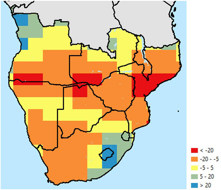
Figure 1. Median projected change in annual precipitation across the ensemble of 7,200 smoothed climate change projections from 2020 to 2050 under the PF scenario, millimeters. Source: Authors calculations, based on Schlosser et al. (2021).

Figure 2 shows the median value of the projected change in the mean daily maximum temperature for 2050 under the PF scenario relative to the baseline period. Coastal areas on both coasts, though especially on the eastern side of the continent, show lower temperature increases than the interior. Coastal region medians are generally below 1.75°C, while the interior is above 1.75°C, with a large portion above 2°C. As we will see in a later section, the highest temperature increase is located in the area that already has the highest temperature. See Schlosser et al. (2021) for a more complete treatment of the climate data.

FIGURE 2

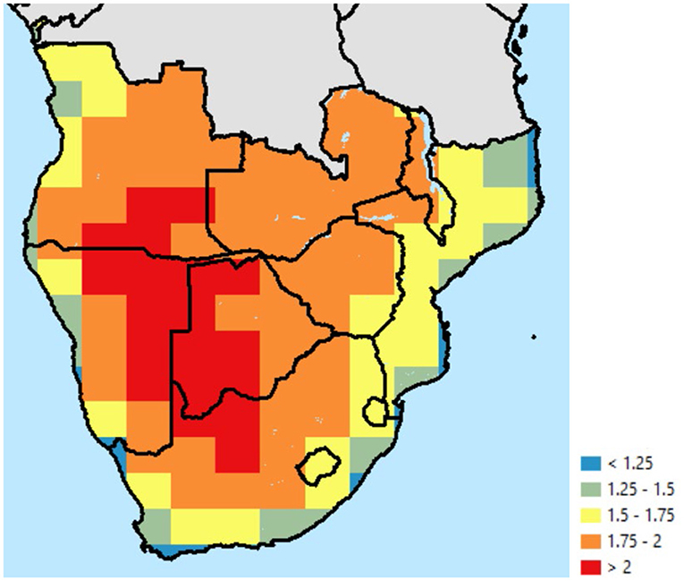
Figure 2. Median projected change in daily maximum temperature across the ensemble of 7,200 smoothed climate change projections from the baseline period (1981–2000) to 2050 under the PF scenario relative to the baseline period, ⁰C. Source: Schlosser et al. (2021).

Historically Observed Climate Patterns

The study area spans arid and semi-arid land in the southwest quadrant of the region up through sub-humid land in the northern and eastern parts of the region. Figure 3 shows the precipitation of the wettest 3 consecutive months. There are many similarities between rainfall in the wet 3 months and annually (not shown), but one difference is that the higher annual rainfall of much of the eastern part of the region—eastern South Africa, southern Mozambique and Lesotho—is not fully reflected in high rainfall in the wet 3 months. This is because the southeastern part of the region has reasonably high rainfall even in their driest months, reflecting a precipitation pattern with little intra-annual variation.

FIGURE 3

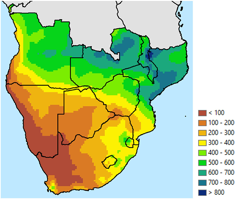
Figure 3. Rainfall in wettest 3 months, millimeters, 1981–2000. Source: Authors' calculations based on Princeton Global Forcings, version 3 [2018, based on Sheffield et al. (2006)].

Many crops are adversely impacted by high temperatures during the growing season. Figure 4 shows the mean daily maximum temperature of the warmest month of the wettest 3 months. If the wettest 3 months reflect the growing season—as it does in most locations—this temperature measure is a good indicator of how stressed crops will become. Schlenker and Roberts (2009) and Lobell et al. (2011a,b) found that temperatures above around 29 or 30 degrees C reduce yields of rainfed maize. Similar results have been found for other grains (Lobell et al., 2011b) and for soybeans (Schlenker and Roberts, 2009; Lobell et al., 2011b). Figure 4 shows that even before the effects of climate change are accounted for, much of the study area is past the optimal temperature for maize cultivation.

FIGURE 4

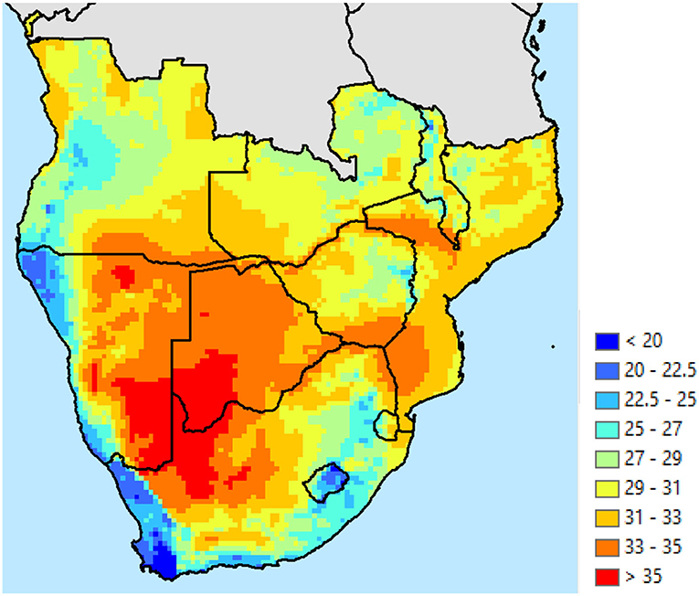
Figure 4. Mean daily maximum temperature for the warmest month in the wettest 3 months, ⁰C, 1981–2000. Source: Authors' calculations based on Princeton Global Forcings, version 3 [2018, based on Sheffield et al. (2006)].

Figure 5 shows that there is significant variation across the region for which months are the wettest 3 months, though most of the area has the wet season spanning the summer months: from November-December-January to February-March-April. In the extreme southwest, there is a relatively small area that with peak rainfall in the winter: mostly May-June-July.

FIGURE 5

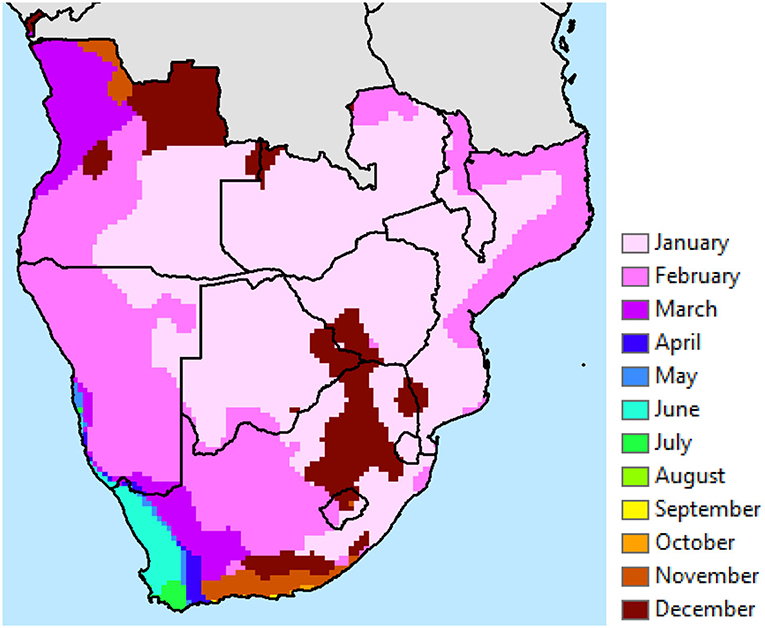
Figure 5. Middle month of wettest 3 months, 1981–2000. Source: Authors' calculations based on Princeton Global Forcings, version 3 [2018, based on Sheffield et al. (2006)].

Figure 6 shows the change in annual precipitation between 1975 and 2015 at each pixel computed by the regressions that generated the “variation deltas.” Most of the study area has gotten drier over that period—though the trends are only statistically significant at the 10% level in a small portion of the area. Parts of Mozambique, in particular, have lost more than 150 millimeters over that 40-year period. Parts of Zambia, Zimbabwe, Botswana, South Africa, and Angola have seen drops of over 100 millimeters. At the same time, extreme northwest Angola has seen an increase of 150 millimeters during that period. While not perfectly matching at every pixel, the trends noted by the regression from historical data are similar to the median changes from the 7,200 climate models for the period between 1990 and 2020 (not pictured). That is, the median of the climate models (PF scenario, in particular) shows a relatively steep decline through 2020, and levels off after 2020.

FIGURE 6

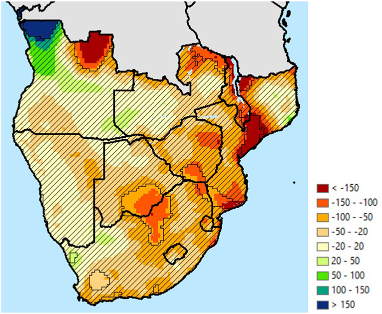
Figure 6. Fourty year trend in change to annual precipitation, 1975–2015, millimeters. Source: Authors, using Princeton Global Forcings daily precipitation. Hash marks show areas with <10% joint statistical significance on the sum of the parameters associated with yr and yr 75 from Equation (1).

Variation-Augmented Climates

From the pool of 68 independent meteorological years that were computed using the PGF historical weather dataset, we took 5,100 random draws with replacement and used those draws to give 100 51-year collections of climate variation deltas that we could use to add to the smoothed climate change data to give variation augmented climate change data. The distribution of the precipitation draws for the wettest 3 months aggregated to the country level is found in Figure 7. We see that Botswana, Namibia, Zimbabwe, Eswatini and to a lesser extent, South Africa, have longer right tails than left. Malawi and Zambia have longer left tails. Mozambique, Lesotho, and Angola are mostly even.

FIGURE 7

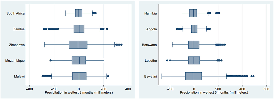
Figure 7. Variation in historical precipitation of the wettest 3 months by country based on detrended monthly data, 1948–2016. Source: Authors' calculations based on Princeton Global Forcings, version 3 [2018, based on Sheffield et al. (2006)]. For box and whisker plots, the box is bounded by the 25th and 75th percentiles, with the mid-line inside the box showing the median. The length from the 25th to the 75th percentile is called the inter-quartile range (IQR). The endpoint of the whiskers is the point that just lies within a distance of 1.5 times the IQR from the ends of the boxes. Any point beyond the whiskers is plotted individually.

Figure 8 shows the distribution of temperature deltas derived from the detrended PGF data converted to meteorological years and drawn for 100 51-year intervals. These were aggregated from pixel to national level. Eswatini and Namibia appear to have longer left tails (greater uncertainty toward cooler temperatures) when measured from the median value. The other countries appear to be mostly balanced.

FIGURE 8

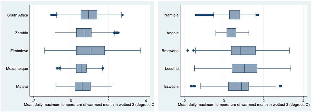
Figure 8. Variation in historical mean daily maximum temperature for the warmest month of the wettest 3 months by country from detrended monthly data, 1948–2016. Source: Authors' calculations based on Princeton Global Forcings, version 3 [2018, based on Sheffield et al. (2006)]. For box and whisker plots, the box is bounded by the 25th and 75th percentiles, with the mid-line inside the box showing the median. The length from the 25th to the 75th percentile is called the inter-quartile range (IQR). The endpoint of the whiskers is the point that just lies within a distance of 1.5 times the IQR from the ends of the boxes. Any point beyond the whiskers is plotted individually.

Using the 100 51-year collections of variation deltas, we add them to the 7,200 smoothed climate change projections for each scenario, to get 720,000 variation-augmented climate change projections per emissions scenario as our complete set of possibilities. With such large numbers, it enables us to examine the full statistical distributions of future climate. In particular, given increasing uncertainty in climate over time, skewness in most climate uncertainties and in some of the variability from historical weather, it is not very obvious what the combined distributions will look like. Studying them, as well as using them to inform crop models and hydrological models in companion papers, will allow us to better understand the fuller cost of climate change, including valuation of shocks, which in turn will help us more accurately value investments to mitigate the costs of climate change, including investments in agricultural research, crop insurance, infrastructure, irrigation, storage, and social protection.

In the left graph of Figure 9, we see the rainfall distribution for the wettest 3 months averaged across Zambia using 9 years of annual data for each plot on the graph¹. The first thing to note is the large difference between the spread of the smoothed climate—which is the uncertainty across about the mean climate given an emissions scenario—compared to that of the variation-augmented climate—which combines both the uncertainty and the inter-annual variation. It shows that the inter-annual rainfall variation is larger than the uncertainty (as can be seen by the difference between the right and left tails of the smoothed climate from the right and left tails of the variation-augmented climate), though by 2060s under PF the contribution of each component is more even since the uncertainty over the magnitude of the mean changes to climate is fairly large by then.

FIGURE 9

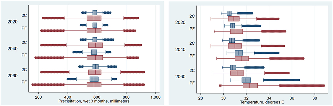
Figure 9. Uncertainty and variation in future precipitation and temperature for Zambia. Source: Authors' calculations. Values are for total precipitation during the wettest 3 months and the mean daily maximum temperature for the warmest month during the wettest 3 months of the year for each pixel, for the given decade, aggregated to the country level. For box and whisker plots, the box is bounded by the 25th and 75th percentiles, with the mid-line inside the box showing the median. The length from the 25th to the 75th percentile is called the inter-quartile range (IQR). The endpoint of the whiskers is the point that just lies within a distance of 1.5 times the IQR from the ends of the boxes. Any point beyond the whiskers is plotted individually. Blue is for the smoothed climate projections. Red is for the variation-enhanced climate projections.

The smoothed climate box and whiskers plots can be important for planning and investing purposes because it gives some idea of the likelihood surrounding a particular future. Often too little is understood about the degree of uncertainty, which can result in poor investments and planning for an outcome that might not actually happen. In some cases, policymakers have been told by researchers with limited access to models that there will be less precipitation in the future, and as a result, investments might have been made reflecting that belief. Once the uncertainty is properly accounted for, information about the distribution of climate futures could lead to a more nuanced and ultimately more helpful investment plan and policy response.

The distributions for the two emissions scenarios are very similar in the 2020s, but by the 2060s the uncertainty and variation is slightly larger for PF than for 2C, with the PF notably having a longer left tail. Additionally, it appears that the left tails of the variation-augmented climate distributions are slightly longer than the right tails, which implies that drought extreme events are projected to be stronger (in terms of distance from the median) than flood extreme events.

The right graph of Figure 9 shows the distribution of the mean daily maximum temperature for the warmest month of the wet 3 months for Zambia. We note several differences from what we noted with precipitation. First, uncertainty concerning the mean of the temperature measure has a relatively stronger influence when compared to the corresponding inter-annual variability than for what we observed with precipitation. Second, we see that unlike precipitation, for which the medians changed very little, with temperature the medians are rising, and they rise much more with PF than with 2C. The right tail grows faster over time than the median does, and the left tail does not change much over time at all. This is potentially bad news for agriculture, since for most crops, productivity drops off rapidly at higher temperatures.

More specifically, looking at the 2060s and comparing the two variation-augmented plots in Figure 9, the medians for the high emissions scenario is roughly 1°C higher than for the low emissions, but the extreme part of the tails have a 3°C difference. This is just one indicator of how much more severe climate extreme events could become in the future. It can help us see the importance of reducing GHG emissions globally even now, because it foreshadows the potential cost of unconstrained emissions.

In balance, however, it could be that even with high emissions, the future climate mean could be realized as one of the more optimistic models, in which case the crisis could be only minor. In the 2C emissions scenario, the median in the 2060s is 1.5°C above that of the 2020s. Such a rise would be harmful to agriculture, but clearly not as harmful as one of the hotter climate models tells us it could be.

We also graphed the precipitation distributions for other countries (see Supplementary Material) and noted the skewness of each. We found that Angola, Botswana, Namibia, and Eswatini had long tails to the right. That is, the model extremes were higher on the high rainfall end than on the low rainfall end. At the same time, Mozambique, Malawi, Zambia, Lesotho, South Africa, and Zimbabwe had much longer tails to the left, favoring bigger dry extremes.

Table 1 summarizes the median changes in climate and the range of combined uncertainty and inter-annual variation of precipitation during the wettest 3 months by pixel and aggregated to the national level. Table 1 confirms that changes in the median across decades and across emissions scenarios is very small in every single nation in the study area.

TABLE 1

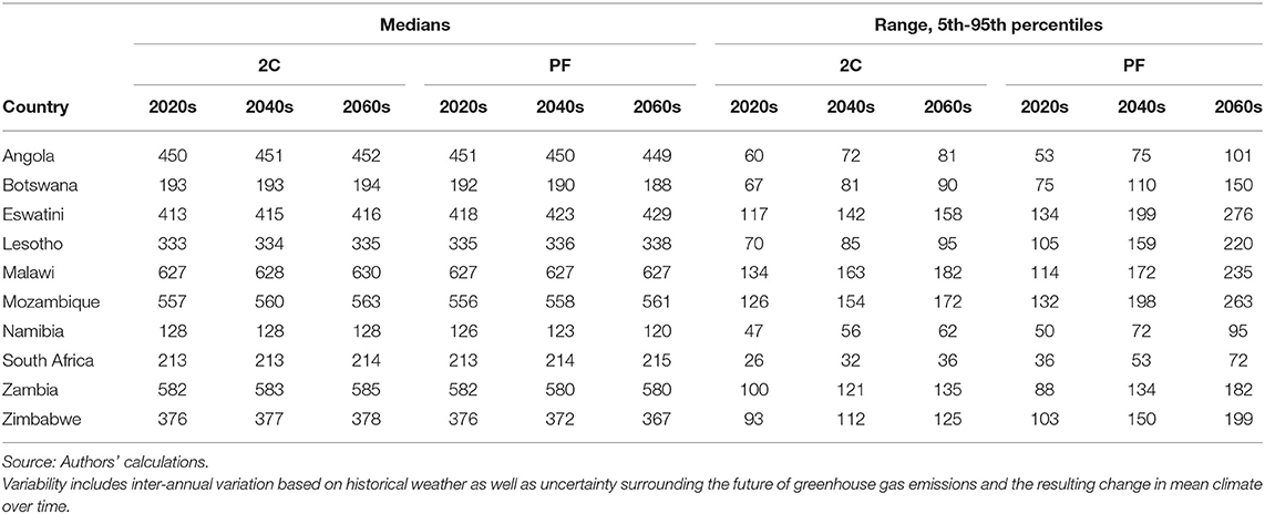
Table 1. Median precipitation and variation for the wettest 3 months across climate models and multiple years in selected decades, in millimeters.

The second thing we notice in Table 1 is that the range of uncertainty rises across decades given any emissions scenario. Third, we see that the increase in uncertainty over time is much greater for the higher emissions scenario, with the range twice as large in South Africa for the “PF” compared to the “2C” in the 2060s, though only 25 percent larger in the case of Angola. We also see that the range of uncertainty can be quite large relative to the median. In the case of the “PF” scenario for Zimbabwe in the 2060s, the range from the 5th to the 95th percentile is 54 percent of the median rainfall.

Table 2 shows the distribution across countries for the variation-augmented climate change for the mean daily maximum temperature for the warmest month of the wettest 3 months for each pixel. Unlike the case for precipitation in which the median did not change much across decades and across emissions scenarios, we note that across all countries, temperatures are projected to rise. However, for the lower emissions “2C” scenario, the changes are small. Most countries are projected to experience only a 0.2°C increase over the next 20 years, followed by a 0.1°C increase in the following 20 years.

TABLE 2

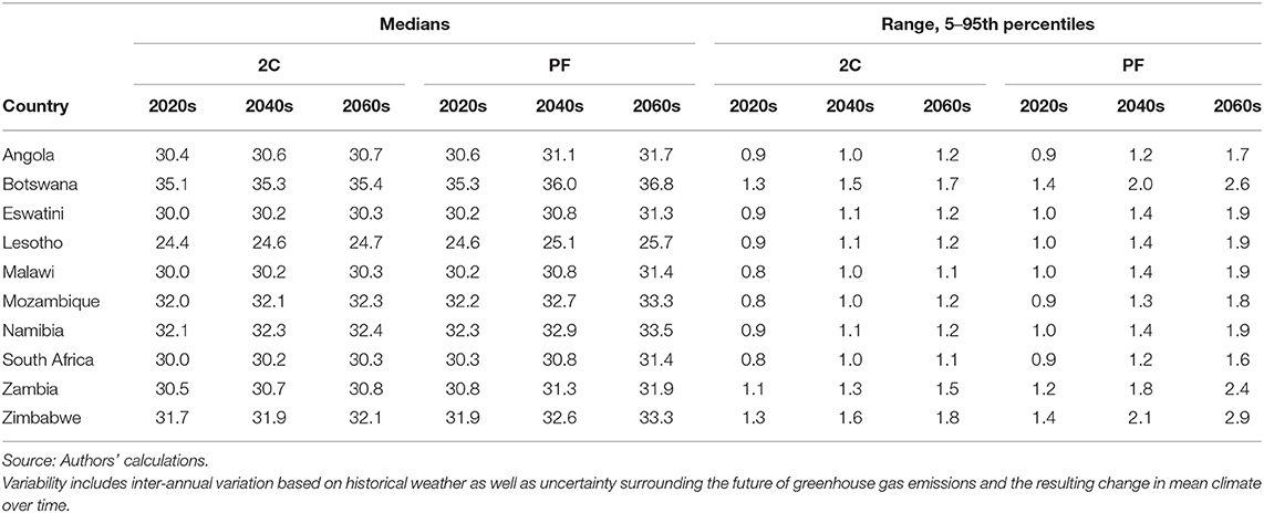
Table 2. Median value for mean daily maximum temperature and variation during the wettest 3 months across climate models and multiple years in selected decades, in ⁰C.

However, with the higher emissions “PF” scenario, temperatures are projected to rise between 0.5° and 0.7°C in the next 20 years, depending upon the country. And between the 2020s and the 2060s, temperatures are projected to rise 1.1° to 1.5°C. Under both scenarios, the increases are in addition to the increases already experienced since the 1970s.

As noted for ranges in climate uncertainty and inter-annual variability for precipitation, the ranges for temperature also increase through time and are larger for the higher emissions scenarios. As for the skewness in the uncertainty about temperature change, all 10 countries have longer right tails than left. Referring to the values used to construct Table 2, the median to 95th percentile range for Zambia and Zimbabwe is at least 90 percent larger than the 5th to median range. And for Botswana and Malawi it is around 70 percent larger. For the other 6 countries, the difference ranges from 20 percent to 45 percent.

Graphs for the distributions in Tables 1, 2 are found in Supplementary Figures 1, 2. These figures not only show the skewness of the data for every year between 2020 and 2069, but they also show that for some countries, the distribution often has more than one peak, similar to what is seen in bivariate normal distributions. Supplementary Figure 3 contains precipitation graphs and Supplementary Figure 4 contains temperature graphs similar to those in Figure 9 for the other 9 countries of the Southern Africa study area.

Even though we noted in Figure 9 that there were only little changes in the left-tail of the precipitation projections in the future for Zambia, we look further at the tails in Table 3, focusing on the frequency of relatively rare 1-in-100-year events. Table 3 has data for not only Zambia but for all 10 countries in the study area. It has data on both the dry year and wet year events, using the 2020s and the low emissions scenario as the baseline level, and seeing what the new frequency is for baseline occurrence.

TABLE 3

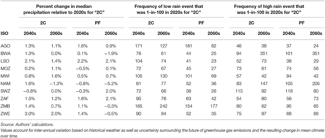
Table 3. Change in frequency of very high and very low precipitation years for the wet 3 months of the year.

The problem with reading box and whiskers plots like those in Figure 8 is that because of the size of the dots in the plot, it is difficult to see how thick the tails are. However, when we look at Table 3 and using the 1-in-100-year low rainfall event during the wet season for the 2020s as a baseline to measure against, we see that although the tail appeared to be moving leftward over time, it actually was moving rightward for Zambia. 1-in-100-year dry events will become rarer there, occurring once every 242 years by the 2060s under 2C and once every 177 years by the 2060s under PF. Zambia is not unique in having such events become rarer: Angola and Malawi also have the dry year extremes become rarer under 2C in both the 2040s and 2060s, though not true by the 2060s under the PF scenario.

More common are the increases in the occurrence of rare dry years, as seen especially under the PF scenario in the 2060s. Lesotho, Botswana, Eswatini, and Mozambique all will expect the 1-in-100-year dry events to occur 4 times more frequently by then. Namibia, Zimbabwe, and South Africa will see them occurring 2.5 times as frequently.

Figure 10 shows the pixel-level changes in frequency of 20-year events by the 2060s under the REF scenario. Northwestern Angola will see dry events less frequently in the 2060s under climate change with the REF scenario, while southern Angola will see them occur roughly twice as often as the baseline 1981–2000 climate. Much of Zambia will have modest increases in dry years, while much of the rest of the study area will see dry years occur about twice as often. The parts of coastal Namibia that appear to have an increased frequency of 4 times is in a very dry area, and the increase reflects a quantitatively small decline.

FIGURE 10

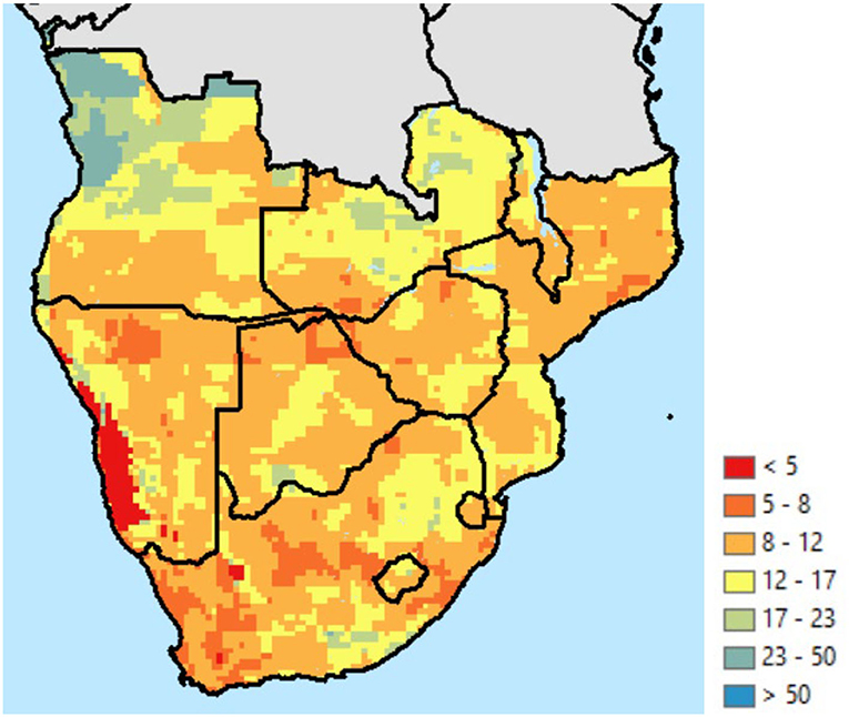
Figure 10. Frequency of 20-year low-rainfall events under climate change, REF scenario, 2060s (baseline 2020s 2C). Source: Authors.

Table 3 also has information on the occurrence of 1-in-100-year wet events in the wet season. By the 2060s, Botswana will be much less likely to experience a rare extremely wet year, only seeing it occur once every 351 years. On the other hand, by the 2060s under the PF scenario, Angola will experience them 4 times more frequently, Lesotho more than 3 times as often, and Malawi roughly 2.5 times as often.

Figure 11 shows the frequency of high-rainfall, 20-year events by the 2060s under the REF emissions scenario. Frequency triples and quadruples in northeastern South Africa, and doubles in much of the eastern coast of South Africa, southern Mozambique and Zimbabwe, northern Zambia, and eastern Botswana, and north and central Angola. Namibia's large increase along the coast is in a low rainfall area and the increase is quantitatively small.

FIGURE 11

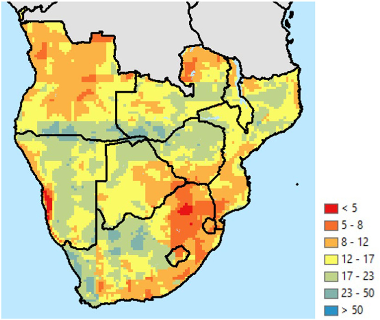
Figure 11. Frequency of 20-year high-rainfall events under climate change, REF scenario, 2060s (baseline 2020s 2C). Source: Authors.

Table 4 shows the results of the same kind of analysis except for mean daily maximum temperature of the warmest month of the wettest 3 consecutive months—and in absolute change in temperature in °C rather than in percent change. The largest increases occur for the high emissions scenario by the 2060s, with values averaging around a 0.8°C increase over the 2020s and a 0.5°C increase relative to the 2040s.

TABLE 4

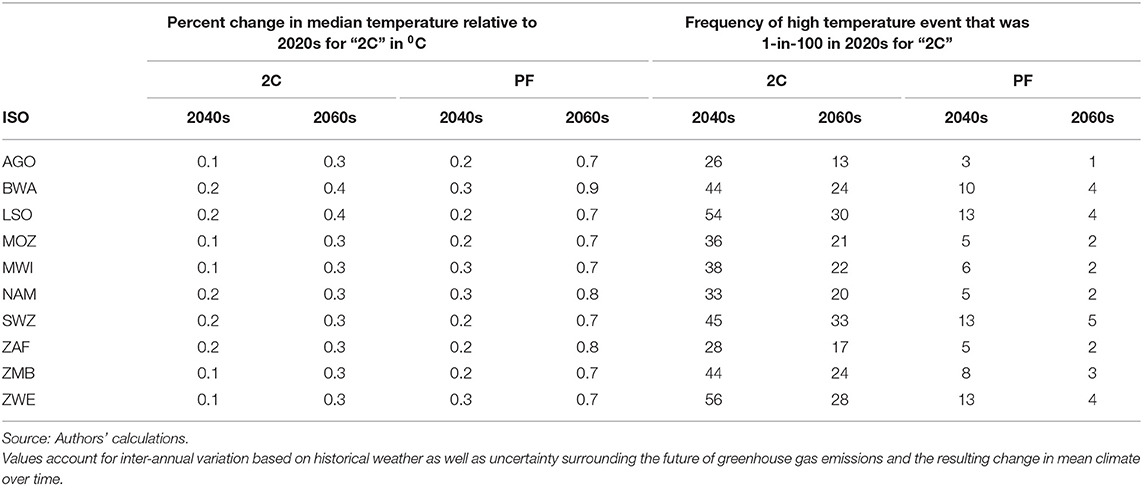
Table 4. Change in frequency of very high temperature years for the wet 3 months of the year.

However, what is of greatest concern is the frequency of extreme high temperature events. Events that happen every 1-in-100 years will become commonplace by the 2060s, if the PF scenario proves to be correct. For Angola, this kind of event will occur every year, though for Eswatini it will only occur on average every fifth year.

On the other hand, if emissions rates can be lowered, by the 2060s, 1-in-100-year events will occur only once every 13 years (in the case of Angola) or even less frequently−1-in-33 years in the case of Eswatini. Even by the 2040s under the higher emissions scenario, the frequency of extreme heat events will become common, ranging from every 3 years for Angola to every 13 years for several countries (Lesotho, Eswatini, and Zimbabwe).

Making such events much more common will create challenges for farmers in a number of ways. We mentioned two of them: lower yields due to heat-stress and lower livestock productivity due to heat stress. It also will lower productivity of labor, because people also suffer from heat stress, and will have negative health consequences, particularly for seniors and those who are malnourished or sick. It may also lower the efficiency of farm machinery, since engines and moving parts are subject to stress under higher temperatures.

Discussion

In this paper we described the development of smoothed climate ensembles (Schlosser et al., 2021) and their subsequent enhancement with inter-annual variation derived from historical weather in such a way that we were able to consider the full-range of effects of climate change on ten countries of Southern Africa. By augmenting the ensemble of smoothed climate change projections with inter-annual variation derived from historical observations in the manner used here, we were able to assess how the frequency and magnitude of precipitation and temperature extremes might change over time, starting with projections at a fine resolution that were then aggregated to the national and regional levels.

The fine-scale analysis together with the focus on low-frequency weather events allows for more detailed sub-national planning that together with linking to other models could allow for developing targeted investments that could be of great benefit to farmers and local planners dealing with infrastructure and energy.

Because the MIT-IGSM dataset used in this study spanned all of continental Africa and the PGF historical weather dataset provides global gridded weather data (as do a number of other datasets), the methods in this study can readily be applied to all other countries in Africa. Furthermore, while there are many advantages of using 7,200 climate models for Africa (such as providing a more complete distribution of climate futures), it would be possible to use fewer models for applications on other continents, taking advantage of the suites of downscaled models provided by CCAFS (Navarro-Racines et al., 2020) or WorldClim (Fick and Hijmans, 2017), for two examples.

This paper focused on the weather during the 3 wettest consecutive months for each pixel because we were primarily concerned with how climate change will impact the agricultural sector. We discovered that median precipitation is not projected to change much. However, largely because of an increase in uncertainty under climate change, the frequency of both extreme high precipitation and extreme low precipitation events will increase.

The largest changes will occur with temperature, which will rise at the median, but will rise by even more in the high temperature tails of the distributions. Furthermore, we discovered large differences between the lower emissions scenario and the higher emissions scenario.

While many will find the results regarding frequency of extreme weather events of interest in their own right, the authors were interested in accounting for climate uncertainty and inter-annual variability for related analyses of irrigation, hydropower, and agriculture for the region. Findings for South Africa are in Arndt et al. (2021) and for the agricultural impact on the Southern Africa region, results can be found in a companion article in this special issue (Thomas et al., 2022).

Regarding agricultural adaptation to climate change, it is likely that spontaneous adaptation will occur at the farm and household level, even without government assistance. For example, farmers may be able to

▪ Move locations of their farms within the country to areas with lower mean temperatures.

▪ Change crops or crop varieties to ones that are more heat resistant.

▪ Shift their planting months slightly to months with cooler temperatures and not too-diminished levels of rainfall.

▪ Build shelters or plant trees to provide shade for their livestock. And with sufficient power availability and in conditions where it makes economic sense, fans and air-conditioning can be used.

▪ Shift outdoor work to cooler hours of the day or possibly even in the night or early morning.

Nevertheless, policy makers can do things to assist farmers in their efforts to adapt. These include

▪ Investment in developing cultivars and livestock that are heat resistant.

▪ Investment in irrigation (there is some evidence that irrigation cools temperatures in the cropping zone and that irrigated crops produce higher yields than rainfed crops because most years the rainfall is suboptimal for maximalyields).

▪ Consider whether there are cooler parts of the country that could be developed without adverse environmental impacts, and assist with legislation and infrastructure to facilitate voluntary movement of farmers to those areas.

▪ Commit to mitigation of GHG emissions and work in bilateral and global forums to encourage all nations to contribute.

For future studies, alternative methods might be used to produce inter-annual variability measures that allow for a larger subset of variation deltas to choose from or which better preserve inter-annual correlation. Unrelated to the manner in which the variation deltas are drawn, it would also be of interest to investigate the impact of increases in the variability of precipitation, given that several authors have argued for the likelihood of experiencing increased weather variability under climate change (Pendergrass et al., 2017; Bathiany et al., 2018; van der Wiel and Bintanja, 2021).

Data Availability Statement

The raw data supporting the conclusions of this article will be made available by the authors, without undue reservation.

Author Contributions

TT was the lead writer of this paper and developed the method of augmenting the smoothed climate change projections with inter-annual variation. CS generated the future climate data. KS provided overall guidance and additional checks, particularly for precipitation and PET. CA served as principal investigator of the project and consulted on methodology and use of his Gaussian quadrature routine. RR consulted on daily weather construction. All authors contributed to the article and approved the submitted version.

Funding

We are grateful for support from the CGIAR Research Program on Policies, Institutions, and Markets (PIM); the CGIAR Research Program on Water, Land and Ecosystems (WLE); the One CGIAR Initiative on Foresight and Metrics to Accelerate Food, Land, and Water Systems Transformation; and the National Treasury, Republic of South Africa.

Conflict of Interest

The authors declare that the research was conducted in the absence of any commercial or financial relationships that could be construed as a potential conflict of interest.

Publisher's Note

All claims expressed in this article are solely those of the authors and do not necessarily represent those of their affiliated organizations, or those of the publisher, the editors and the reviewers. Any product that may be evaluated in this article, or claim that may be made by its manufacturer, is not guaranteed or endorsed by the publisher.

Supplementary Material

The Supplementary Material for this article can be found online at: https://www.frontiersin.org/articles/10.3389/fclim.2022.787721/full#supplementary-material

Footnotes

1. ^The 2020s span 2021-2029, the 2040s span 2040-2048, and the 2060s span 2060-2068.

References

Arndt, C., Gabriel, S., Hartley, F., Strzepek, K. M., and Thomas, T. S. (2021). “Climate change and the green transition in South Africa,” in The Oxford Handbook of the South African Economy, eds A. Oqubay, F. Tregenna, I. Valodia (Oxford: Oxford University Press), p. 323–345. doi: 10.1093/oxfordhb/9780192894199.013.16

CrossRef Full Text | Google Scholar

Arndt, C. P., Chinowsky, C., Fant, C., Paltsev, S., Schlosser, C. A., Strzepek, K., et al. (2019). Climate change and developing country growth: the cases of Malawi, Mozambique, and Zambia. Clim. Change 154, 335–349. doi: 10.1007/s10584-019-02428-3

CrossRef Full Text | Google Scholar

Bathiany, S., Vasilis, D., Marten, S., and Lenton, T. M. (2018). Climate models predict increasing temperature variability in poor countries. Sci. Adv. 4:eaar5809. doi: 10.1126/sciadv.aar5809

PubMed Abstract | CrossRef Full Text | Google Scholar

Belcher, S. E., Hacker, J. N., and Powell, D. S. (2005). Constructing design weather data for future climates. Building Serv. Eng. Res. Technol. 26, 49–61. doi: 10.1191/0143624405bt112oa

CrossRef Full Text | Google Scholar

Chen, D., Rojas, M., Samset, B. H., Cobb, K., Diongue Niang, A., Edwards, P., et al. (2021). “Framing, context, and methods,” in Climate Change 2021: The Physical Science Basis. Contribution of Working Group I to the Sixth Assessment Report of the Intergovernmental Panel on Climate Change, eds V. Masson-Delmotte, P. Zhai, A. Pirani, S. L. Connors, C. Péan, S. Berger, N. Caud, Y. Chen, L. Goldfarb, M. I. Gomis, M. Huang, K. Leitzell, E. Lonnoy, J. B. R. Matthews, T. K. Maycock, T. Waterfield, O. Yelekçi, R. Yu and B. Zhou (Cambridge; New York, NY: Cambridge University Press), p. 1–215.

Google Scholar

Collins, M., Knutti, R., Arblaster, J., Dufresne, J.-L., Fichefet, T., Friedlingstein, P., et al. (2013). “Long-term climate change: projections, commitments and irreversibility,” in Climate Change 2013: The Physical Science Basis. Contribution of Working Group I to the Fifth Assessment Report of the Intergovernmental Panel on Climate Change, eds T. F. Stocker, D. Qin, G. K. Plattner, M. Tignor, S. K. Allen, J. Boschung, A. Nauels, Y. Xia, V. Bex, P. M.and Midgley (Cambridge; New York, NY: Cambridge University Press), p. 1029–1136.

Google Scholar

Fant, C., Gebretsadik, Y., McCluskey, A., and Strzepek, K. (2015). An uncertainty approach to assessment of climate change impacts on the Zambezi River Basin. Clim. Change 130, 35–48. doi: 10.1007/s10584-014-1314-x

CrossRef Full Text | Google Scholar

FAO IFAD, UNICEF, WFP, and WHO. (2020). The State of Food Security and Nutrition in the World (2020). Transforming food systems for affordable healthy diets. Rome, FAO.

Google Scholar

Fick, S. E., and Hijmans, R. J. (2017). WorldClim 2: new 1-km spatial resolution climate surfaces for global land areas. Int. J. Climatol. 37, 4302–4315. doi: 10.1002/joc.5086

CrossRef Full Text | Google Scholar

IPCC (2013). “Annex I: Atlas of Global and Regional Climate Projections,” in Climate Change 2013: The Physical Science Basis. Contribution of Working Group I to the Fifth Assessment Report of the Intergovernmental Panel on Climate Change, eds G. J. van Oldenborgh, M. Collins, J. Arblaster, J. H. Christensen, J. Marotzke, S. B. Power, M. Rummukainen, and T. Zhou (New York, NY; Cambridge: Cambridge University Press), p. 1311–1393.

Google Scholar

IPCC (2021). “Summary for policymakers,” in Climate Change 2021: The Physical Science Basis. Contribution of Working Group I to the Sixth Assessment Report of the Intergovernmental Panel on Climate Change, eds V. Masson-Delmotte, P. Zhai, A. Pirani, S. L. Connors, C. Péan, S. Berger, N. Caud, Y. Chen, L. Goldfarb, M. I. Gomis, M. Huang, K. Leitzell, E. Lonnoy, J. B. R. Matthews, T. K. Maycock, T. Waterfield, O. Yelekçi, R. Yu, and B. Zhou (Cambridge; New York, NY: Cambridge University Press), p. 1–41.

Google Scholar

Kunreuther, H., Gupta, S., Bosetti, V., Cooke, R., Dutt, V., Ha-Duong, M., et al. (2014). “Integrated risk and uncertainty assessment of climate change response policies,” in Climate Change 2014: Mitigation of Climate Change. Contribution of Working Group III to the Fifth Assessment Report of the Intergovernmental Panel on Climate Change, eds O. Edenhofer, R. Pichs-Madruga, Y. Sokona, E. Farahani, S. Kadner, K. Seyboth, A. Adler, I. Baum, S. Brunner, P. Eickemeier, B. Kriemann, J. Savolainen, S. Schlömer, C. von Stechow, T. Zwickel, and J. C. Minx (Cambridge; New York, NY: Cambridge University Press), p. 151–206.

Google Scholar

Lee, J. Y., Marotzke, J., Bala, G., Cao, L., Corti, S., Dunne, J. P., et al. (2021). “Future global climate: scenario-based projections and near-term information,” in Climate Change 2021: The Physical Science Basis. Contribution of Working Group I to the Sixth Assessment Report of the Intergovernmental Panel on Climate Change, eds V. Masson-Delmotte, P. Zhai, A. Pirani, S. L. Connors, C. Péan, S. Berger, N. Caud, Y. Chen, L. Goldfarb, M. I. Gomis, M. Huang, K. Leitzell, E. Lonnoy, J. B. R. Matthews, T. K. Maycock, T. Waterfield, O. Yelekçi, R. Yu and B. Zhou (Cambridge: Cambridge University Press), p. 4–195.

Google Scholar

Lobell, D. B., Bänziger, M., Magorokosho, C., and Bindiganavile, V. (2011a). Nonlinear heat effects on African maize as evidenced by historical yield trials. Nat. Climate Change 1, 42–45. doi: 10.1038/nclimate1043

CrossRef Full Text | Google Scholar

Lobell, D. B., Schlenker, W., and Costa-Roberts, J. (2011b). Climate trends and global crop production since (1980). Science 333, 616–620. doi: 10.1126/science.1204531

PubMed Abstract | CrossRef Full Text | Google Scholar

Navarro-Racines, C., Tarapues, J., Thornton, P., Jarvis, A., and Ramirez-Villegas, J. (2020). High-resolution and bias-corrected CMIP5 projections for climate change impact assessments. Sci. Data 7:7. doi: 10.1038/s41597-019-0343-8

PubMed Abstract | CrossRef Full Text | Google Scholar

Pendergrass, A. G., Knutti, R., Lehner, F., et al. (2017). Precipitation variability increases in a warmer climate. Sci. Rep. 7:17966. doi: 10.1038/s41598-017-17966-y

PubMed Abstract | CrossRef Full Text | Google Scholar

Reilly, J., Chen, Y. H., Sokolov, A., Gao, X., Schlosser, A., Morris, J., et al. (2018). MIT Joint Program on the Science and Policy of Global Change. Available online at: https://globalchange.mit.edu/outlook.

Google Scholar

Schlenker, W., and Roberts, M. J. (2009). Nonlinear temperature effects indicate severe damages to U.S. crop yields under climate change. Proc. Natl. Acad. Sci. U.S.A. 106, 15594–15598. doi: 10.1073/pnas.0906865106

PubMed Abstract | CrossRef Full Text | Google Scholar

Schlosser, C. A., Gao, X., Strzepek, K., Sokolov, A., Forest, C. E., Awadalla, S., and Farmer, W. (2012). Quantifying the likelihood of regional climate change: a hybridized approach. J. Climate 26, 3394–3414. doi: 10.1175/JCLI-D-11-00730.1

CrossRef Full Text | Google Scholar

Schlosser, C. A., Andrei, S., Ken, S., Tim, T., Xiang, G., and Channing, A. (2020). The changing nature of hydroclimatic risks across South Africa. Joint Program Rep. Series Report 342. Available online at: http://globalchange.mit.edu/publication/17483.

Google Scholar

Schlosser, C. A., Andrei, S., Ken, S., Tim, T., Xiang, G., and Channing, A. (2021). The changing nature of hydroclimatic risks across South Africa. Climatic Change 168. doi: 10.1007/s10584-021-03235-5

CrossRef Full Text | Google Scholar

Schlosser, C. A., and Strzepek, K. (2015). Regional climate change of the greater Zambezi River basin: a hybrid assessment. Climatic Change 130, 9–19 doi: 10.1007/s10584-014-1230-0

CrossRef Full Text | Google Scholar

Seneviratne, S. I., Nicholls, N., Easterling, D., Goodess, C. M., Kanae, S., Kossin, J., et al. (2012). “Changes in climate extremes and their impacts on the natural physical environment,” in Managing the Risks of Extreme Events and Disasters to Advance Climate Change Adaptation, eds C. B. Field, V. Barros, T. F. Stocker, D. Qin, D. J. Dokken, K. L. Ebi, M. D. Mastrandrea, K. J. Mach, G. K. Plattner, S. K. Allen, M. Tignor, and P. M. Midgley. A Special Report of Working Groups I and II of the Intergovernmental Panel on Climate Change (IPCC) (Cambridge; New York. NY: Cambridge University Press), p. 109–230. doi: 10.1017/CBO9781139177245.006

CrossRef Full Text | Google Scholar

Seneviratne, S. I., Zhang, X., Adnan, M., Badi, W., Dereczynski, C., Di Luca, A., et al. (2021). “Weather and climate extreme events in a changing climate,” in Climate Change 2021: The Physical Science Basis. Contribution of Working Group I to the Sixth Assessment Report of the Intergovernmental Panel on Climate Change, eds V. Masson-Delmotte, P. Zhai, A. Pirani, S. L. Connors, C. Péan, S. Berger, N. Caud, Y. Chen, L. Goldfarb, M. I. Gomis, M. Huang, K. Leitzell, E. Lonnoy, J. B. R. Matthews, T. K. Maycock, T. Waterfield, O. Yelekçi, R. Yu and B. Zhou (Cambridge: Cambridge University Press), p. 11–345.

PubMed Abstract | Google Scholar

Sheffield, J., Goteti, G., and Wood, E. F. (2006). Development of a 50-yr high-resolution global dataset of meteorological forcings for land surface modeling. J. Climate 19, 3088–3111. doi: 10.1175/JCLI3790.1

CrossRef Full Text | Google Scholar

Sokolov, A., Kicklighter, D., Schlosser, A., Wang, C., Monier, E., Brown-Steiner, B., et al. (2018). Description and evaluation of the MIT Earth System Model (MESM). J. Adv. Model. Earth Syst. 10, 1759–1789. doi: 10.1002/2018MS001277

CrossRef Full Text | Google Scholar

Thomas, T. S., Robertson, R. D., Strzepek, K., and Arndt, C. (2022). Extreme events and production shocks for key crops in Southern Africa under climate change. Front. Clim. 4, 787582. doi: 10.3389/fclim.2022.787582

CrossRef Full Text | Google Scholar

Thome, K., Birgit, M., Kamron, D., and Cheryl, C. (2018). International Food Security Assessment, 2018-2028, GFA-29, U.S. Department of Agriculture, Economic Research Service, June.

Google Scholar

van der Wiel, K., and Bintanja, R. (2021). Contribution of climatic changes in mean and variability to monthly temperature and precipitation extremes. Commun. Earth Environ. 2:1. doi: 10.1038/s43247-020-00077-4

CrossRef Full Text | Google Scholar