Extreme Events and Production Shocks for Key Crops in Southern Africa Under Climate Change

Many studies have estimated the effect of climate change on crop productivity, often reflecting uncertainty about future climates by using more than one emissions pathway or multiple climate models, usually fewer than 30, and generally much fewer, with focus on the mean changes. Here we examine four emissions scenarios with 720,000 future climates per scenario over a 50-year period. We focus on the effect of low-frequency, high-impact weather events on crop yields in 10 countries of Southern Africa, aggregating from nearly 9,000 25-kilometer-square locations. In the highest emissions scenario, median maize yield is projected to fall by 9.2% for the region while the 5th percentile is projected to fall by 15.6% between the 2020s and 2060s. Furthermore, the frequency of a low frequency, 1-in-20-year low-yield event for rainfed maize is likely to occur every 3.5 years by the 2060s under the high emissions scenario. We also examine the impact of climate change on three other crops of considerable importance to the region: drybeans, groundnuts, and soybeans. Projected yield decline for each of these crops is less than for maize, but the impact varies from country to country and within each country. In many cases, the median losses are modest, but the losses in the bad weather years are generally much higher than under current climate, pointing to more frequent bouts with food insecurity for the region, unless investments are made to compensate for those production shocks.

Introduction

A number of authors have investigated the likelihood of experiencing increased climate variability under climate change (Pendergrass et al., 2017; Bathiany et al., 2018; van der Wiel and Bintanja, 2021). Fewer have investigated the implications of uncertainty regarding emissions pathways coupled with uncertainty concerning the effects on future climate possibilities while accounting for inter-annual variation. Here, we investigate the implications of both climate uncertainty and variability for crop production in Southern Africa. Our motivation is to better understand low-yield events because of their effects on food insecurity.

Most of world's poor and food-insecure people live in rural areas and are smallholder farmers, fishermen, and agricultural laborers (FAO et al., 2018). Their diets consist almost entirely of food produced locally. Weather shocks, therefore, can be extremely disruptive for the nutrition and health of these households, limiting food availability and increasing local market prices, sometimes causing permanent health consequences, especially for young children.

The Sustainable Development Goals (SDGs; see United Nations, 2015) seek to address these issues through various channels. SDG1, ending poverty, targets building resilience of farmers to climate shocks and improving social protection. SDG2, ending hunger and food insecurity, includes a component for doubling the productivity and income of small-scale food producers. Until 2014, household food insecurity had been steadily declining. Since then, the number of food insecure people has risen each year and is projected to continue to rise through the decade, suggesting that the SDGs cannot be achieved by their target date of 2030 (FAO et al., 2020).

Climate change increases the difficulty of meeting the goals by reducing the average yields for most crops and most countries. This phenomenon has been well studied. However, no one has conducted a rigorous analysis on the effect of future climate change on yields in the years with adverse weather shocks. Those years are most vital for the SDGs, because they include the greatest food shortfalls for rural families, thus highlighting the need for effective social protection programs. If the event is sufficiently enduring, severe, and widespread, a regional crisis may ensue as multiple nations struggle to compensate for shortfalls through trade and through substitution of alternative foods (Gaupp et al., 2020).

Understanding the effect of future adverse weather shocks on production would enable governments to develop the capacity needed to address the crisis after it happens or invest beforehand in mitigating measures to reduce the degree of crisis. With sufficient information, even farmers themselves could take steps to mitigate the impact by choosing certain crops, cultivars, and production technologies.

This analysis focuses on 10 countries of Southern Africa, a region in which 44% of the population is food insecure (Thome et al., 2018), in large part due to the frequency of droughts and pests. Thome et al. (2018) estimate that the percent of food insecure will decline over the next 10 years in the region, while the FAO et al. project that the absolute number of food insecure will double in the same period of time (FAO et al., 2020). The difference in direction between the two statistics—one in percent, one in numbers—is partly due to the growing population over that time, but also due to differences in definitions of which countries are part of Southern Africa.

We do detailed analysis on maize, drybeans, groundnuts, and soybeans, key crops for the region, ranking 1, 3, 4, and 6 by total harvested area (Table 1). This article focuses most on maize, largely because it is the region's leading source of calories and protein (followed by wheat in both cases), but we include sections on the other three, as well.

TABLE 1

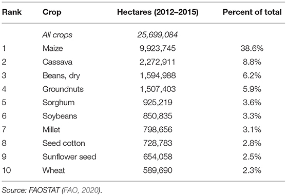
Table 1. Top 10 crops by harvested area in Southern Africa.

Maize production accounts for more than 2.6 times the calories and 2.2 times the amount of protein than wheat and represents roughly 32% of both total calories and proteins consumed in the region (FAO, 2020). Perhaps more importantly, maize represents 41.1% of the harvested area of the region (FAO, 2020), implying that the diets of smallholders may have a much higher proportion of maize than are indicated in the aggregate numbers that include urban areas.

We address the implications of climate change for the frequency and severity of major production shortfalls over the next four decades. As far as we can tell, this is the first focused analysis on low-yield events conducted for any region in the world that used a spatially- and temporally-consistent dataset that was large enough to investigate the behavior of the tails of yield distributions. Burke et al. (2015) tell us that out of approximately 100 studies they reviewed, the median number of climate models used to investigate the effect of climate on agricultural productivity was 2. In this study, we use 720,000 per emissions scenario—almost 3 million total.

Most studies that explore these issues tend to focus on yield variation associated with climate and weather and almost never consider the impact of climate on the changes in the tail of the distribution. Ostberg et al. (2018) use spatially- and temporally consistent data for 4 emissions scenarios (RCPs), 5 GCMs (i.e., climate models), and 5 crop models to build a very sparse emulator. They investigate yield variation but are limited by the number of weather simulations (it appears they only used one weather pathway over a multi-year period). Liu et al. (2021) investigated yield variability of wheat in China due to climate change, but their analysis is limited by the number of climate models (5) and weather simulations (25) used, and the number of sites (8). Chen et al. (2018) analyze the long-term impacts of climate change under 2 emissions scenarios in China, using 4 GCMs and up to 20 weather simulations each. Stuch et al. (2020) compute yields and variability of maize, sorghum, and millet for Sub-Saharan Africa for one emissions scenario and 6 GCMs, but it is not clear that they used a spatially-consistent weather input, which would render any national aggregation incorrect—though their primary objective is at the pixel level. Earlier works focusing on yield variation include Torriani et al. (2007) which examined maize and wheat yield in Switzerland and Thornton et al. (2009), which analyzed maize and drybeans in East Africa.

To investigate these extreme climate-driven low-yield events, we deploy a large suite of potential future smoothed climates (moving averages of precipitation and temperature)—7,200 for each of 4 emissions scenarios. These climate ensembles, labeled hybrid frequency distributions (HFDs), are developed specifically to estimate the distribution of potential climate outcomes to 2060 (Schlosser et al., 2012, 2020, 2021). Further, we overlay these climates with 100 spatially- and temporally-consistent deviations from the mean from historical climate data at each pixel—almost 9,000 pixels of quarter-degree (25-km) resolution—to give 720,000 potential paths for future climates per emissions scenario. Overlaying these 100 sets of data adds in the inter-annual variation that was missing from the smoothed climates. This set of 720,000 weather paths from 2020 to 2069 is taken as the best available estimate of the full distribution of possible growing conditions that farmers may experience over the next four decades. Details of the process used are in a companion article (Thomas et al., 2022).

The large number of climates that account for inter-annual variation allow us to consider extreme events, emphasizing confluences of climate and weather together that are particularly unfavorable to yields. The large number of pixels also allows us to consider impact on yields at various scales. However, computational burdens present considerable barriers. To render the problem tractable, three steps are taken. We deploy an intelligent sampling framework that preserves the moments of key climate outcomes critical to yields out to order three, thereby reducing the number of climate pathways to 455 per emissions scenario. Furthermore, because yields are calculated at pixel level annually to 2069 for multiple crops, soils, and levels of input use, 455 climate pathways remain computationally prohibitive for detailed crops models. To expedite computation of yields, a statistical crop emulator for each of the four focus crops is developed and deployed.

While the process used to compute pixel-based yields was computationally intensive, it is similar to the process used by the international teams that participate in the Agricultural Model Intercomparison and Improvement Project (AgMIP) Gridded Global Crop Model Intercomparison (GGCMI). See for example Müller and Robertson (2014) and Rosenzweig et al. (2014), and more recent work of Ostberg et al. (2018), Franke et al. (2020), Jägermeyr et al. (2021), and Zabel et al. (2021). In some of the research of GGCMI, they use crop model results directly with climates that have both inter-annual variation and uncertainty across multiple models. In others, they use emulator output. The innovation presented in this articles comes in using the methodology with such a large number of climates which allow for more confidence in examining the tail of the distribution which describes the low-yield events that are the main focus of this study.

Materials and Methods

IGSM-HFD Climate Data

The climate ensemble that forms the basis for this analysis provides an opportunity to evaluate not only the distribution of future climates under a given emissions scenario, it enables us to evaluate an arguably complete distribution of abiotic consequences of climate change on crop yields. It is from the MIT Integrated Global System Model (MIT-IGSM, Reilly et al., 2018) which simplifies climates by considering only elevation (vertical) and latitudes so that the computing time is reduced to allow for a wider range of possible patterns of change. In order to expand longitudinally, eighteen GCMs from CMIP5 are used.

There are four emissions scenarios used in the ensemble:

• Reference (REF): There are no explicit emissions mitigation policies anywhere in the world, though it allows for energy policies that lead to some renewable energy and fuel efficiency that are motivated by other reasons besides mitigation.

• Paris Forever (PF): Assumes that countries meet the mitigation targets in their Nationally Determined Contributions (NDCs) and those targets are met throughout the century.

• 2C: Reflects an effort to limit climate change to no higher than a 2°C global average at 2100 through globally coordinated, smoothly rising carbon price. This scenario reflects the uncertainty of the climate response in the MIT Earth System Model (MESM, Sokolov et al., 2018) and leads to an overall probability of achieving the target of 66%.

• 1p5C: Similar to 2C, but targeting a 1.5°C global average at 2100.

The MIT-IGSM produces 400 smoothed climates per emissions scenario, so combining these with the 18 GCMs gives 7,200 hybrid-frequency distributions (which we will generally refer to as “climate models”) per scenario. These provide monthly data from 2020 to 2069 for precipitation and mean daily temperature. The ensemble is described in more detail in in Schlosser et al. (2020, 2021).

Princeton Global Forcings Weather Data

To generate realistic future weathers that are consistent in both space and time, we add historical inter-annual climate variation on top of the smoothed monthly climate change information in the 7,200 climate models. Details are provided in Thomas et al. (2022). The weather data is from the Princeton Global Forcings (PGF) dataset, version 3 (based on Sheffield et al., 2006). This dataset provides daily weather data for a number of weather variables, including the ones relevant to this analysis: precipitation and daily minimum and maximum temperatures. The data spans the period from the beginning of 1948 to the end of 2016. It is at a quarter degree resolution, which in most places reflects rectangles with 25–30 km on each edge. For most of our work we are interested in monthly data, so we aggregate the data, summing the precipitation and computing monthly values for mean daily maximum and mean daily minimum temperatures.

We also use the PGF data to create the baseline climate to add the HFDs to by taking monthly averages from monthly precipitation, daily maximum temperature, and daily minimum temperature at each pixel for the period 1981 to 2000.

Gaussian Quadrature

It is both computer-intensive and time-consuming to perform complex operations on 720,000 weathers. For the purposes of this study, notably modeling crop yields, it was more practical to operate with a subset. The least complicated option would have been to use random sampling to extract the subset. Instead, we decided to follow the methodology of Arndt et al. (2015) and use a Gaussian quadrature (GQ) reduction that allowed us to exactly reproduce the first, second, and third moments of all 720,000 weathers for key regions, time periods, and variables. Using that procedure, we were able to reduce the number of weathers to 455 per emissions scenario while still maintaining representation across the diverse range of possibilities. For the purpose of considering extreme events, a salient advantage of the GQ approach is its tendency to seek out less common (or more extreme) weathers, giving relatively less weight, and choosing relatively few more common weathers and giving those weathers relatively more weight. More detail on generating future climates from the smoothed climates of the MIT-IGSM and the variation provided by the PGF historical data and on the GQ procedure can be found in a companion article (Thomas et al., 2022).

DSSAT Crop Modeling

The Decision Support System for Agrotechnology Transfer (DSSAT) is crop simulation software suite that consists of multiple crop-specific mathematical models (Jones et al., 2003). The models “grow” the crop in daily time increments using daily weather data. In this paper, the weather data is provided by a process that combines the daily weather from the PGF dataset together with the MIT-IGSM, using a subset of climates selected using the Gaussian quadrature sampling. Our DSSAT analysis used soils from Koo and Dimes (2010) which consists of 27 types, of which 18 are found in the study area.

Providing daily weather to DSSAT is usually straightforward. DSSAT has a weather simulator sub-package that generates consistent daily data based on monthly climate statistics provided by the user. However, the daily weather data generated by the weather simulator are not spatially-consistent: the weather in one pixel (location) is not correlated with the weather in a neighboring pixel. Therefore, in order to generate yields that are representative at a higher unit of aggregation, such as the national level, an alternative process needs to be done.

Given that the PGF dataset has daily historical weather data, we are able to generate daily future weather data that exactly reflects the monthly future data that we simulated. However, the storage requirement for daily simulated rainfall and temperature for each pixel in the 10-country study area for the 50 years of the study for 455 climates for each of the 4 emissions scenarios is extremely large. Furthermore, the computational time to generate daily simulated data along with the computational time for the crop model to simulate crop yields based on that daily data make it prohibitive in our case. In order to take advantage of the modeling abilities of DSSAT but not be constrained by the computational challenges of running so many simulations, we decided to build a crop yield emulator.

Building a Crop Yield Emulator

A crop yield emulator is meant to quickly take climate inputs and possibly a few additional variables and generate a corresponding yield for each crop. The emulators are built by regressing yields on monthly climate parameters and other relevant variables (Blanc and Sultan, 2015; Ostberg et al., 2018; Franke et al., 2020), and the parameters estimated in the regression are used to predict yields both in and out of sample.

To generate yield values to use in building the emulators, we sample 1 out of 16 pixels in our study area, using a regular grid with pixels separated by 1 degree. Furthermore, we limit our sampling to simulated climates from the 2020 to 2035 period from the 1p5C emissions scenario (lowest emissions scenario) and for 2054 to 2069 from the REF scenario (highest emissions scenario). This is done to make sure we have weathers reflecting both ends of the spectrum of possibilities, from low temperatures to high temperatures, exploring the feasible bounds for the region both in the present and in the future. For these pixels and particular climates, we produce simulated daily weather corresponding to the 455 climates per emissions scenario selected by the GQ procedure. The daily weather data is passed to DSSAT, which produces the yield at each pixel for a cultivar that is appropriate for the region for each crop in this study. In some of the simulations, we apply two different levels of nitrogen fertilizer so that we would be able to calculate a yield response for fertilizer use.

If actual yield data were available for various locations in the region—and assuming this data could be linked to the corresponding monthly climate data for the growing months—those yields could be used instead of yields from DSSAT. Several authors have used county-level annual yields (Schlenker and Roberts, 2009; Lobell et al., 2011; Dell et al., 2014; Miao et al., 2015; Thomas, 2015) in regressions for their studies of the effect of climate change on crop productivity. However, in addition to that kind of data not being available for our study area, these authors were unable to include variables that would allow estimation of yield response to chemical fertilizer or to atmospheric CO2 fertilization—the latter being limited by CO2 levels being highly correlated to each year (with the year being used to estimate the rate of technological change in agriculture). DSSAT is able to supply yield responses to both.

In order to control for unmeasured influences on yield at each location, authors using historical aggregated yield statistics typically use first differencing or fixed effects rather than a simple cross-sectional approach. However, in our analysis, because we have modeled data, we can control for all location-specific variables in the statistical analysis. That is, when running DSSAT, we fix farm-management practices to be identical at all locations. The only things that differ are the climate and the soils. DSSAT produces the same yield for any two locations in the world if both locations have the same soil and daily climate. Therefore, it is appropriate to forego fixed effects models and instead run cross-sectional regressions for each of the 18 soils in our study area, which we do.

A crop model such as DSSAT can be trained to mimic conditions in a farmer's field with careful observation of management practices, a good knowledge of the soils and cultivar, and an accurate measure of soil starting conditions such as water and nutrient content. When using DSSAT over such a large, heterogeneous area, local conditions cannot be reproduced due to lack of information, so the best generalizations possible are made. However, when using DSSAT—or the corresponding emulator—for this kind of analysis, researchers doing this kind of work trust that by keeping farm management practices constant, they can reasonably predict yield changes due to climate change, which is the goal of the analysis.

One of the advantages of running a separate regression for each soil type rather than including soil parameters in one big regression—unless interaction terms between soils and precipitation is included—is that it allows much more varied response of yield to precipitation based on the soil. Crops grown in soils that retain moisture well would presumably need less precipitation than crops grown in soils that are poor in water retention. The secondary purpose of emulators is to be able to simplify the relationship between climate and yield so that it can be understood more intuitively than the complex processes programmed into crop modeling software.

In the model used to build the emulator for each crop, let m index the month in relationship to the planting date (e.g., the first 30 days after planting is considered month 1); T represent the mean daily maximum temperature for the month; and P represent the total precipitation in the month. In numerous studies of climate impact on agriculture, authors focus almost entirely on some measure of temperature and some measure of precipitation. We opted for using monthly values because they are readily available from climate models. We chose mean daily maximum temperature for the month because we found it to be slightly more intuitive and since it is usually the high temperatures that reduce potential yields. In previous work, we attempted to include an additional temperature measure—mean daily minimum temperature—but because it is highly correlated with the mean daily maximum temperature, it did not lead to very much improvement in the fit of the model.

It would be possible to run regression variables at shorter time intervals than a month, but the advantage of doing that is limited, because only inter-annual variation could be rescaled, since the smoothed MIT-IGSM data came as monthly data. Shorter time intervals also present challenges interpreting the results. Weekly data, for example, would require 4 times as many parameters. It would also be possible to use longer time intervals, such as 2-month, 3-month, or entire growing season values. This would blur some of the impacts of climate on yields since plants change in their reaction to climate depending upon their phase of growth.

We estimate the response function as piecewise-linear in both T and P. A piecewise linear function imposes very little structure onto the yield response except for continuity. This flexible functional form seems to be very important for some crops at high values of precipitation and high and low values of temperature, because lower order polynomials (linear, quadratic, and cubic) can force regressions that generally have few observations at climate extremes to permit very large residuals for such values, as well as predict yields poorly at extreme values.

To define variables to be used for piecewise linear estimation, let z represent either T or P. Divide z into n groups such that z_min < z₁ < z₂ < … < z_n−1 < z_max. Define n-1 new variables z_zk, where k = 1, 2, …, n-1, which are equal to 0 if z < z_k and z – z_k otherwise. For example, if T = 23°C, T₂₀ would be 3 while T₂₅ would be 0. In the emulator developed in this study, we examine values of temperature and precipitation in the region during the cropping months, and choose to divide monthly precipitation into groups divided at 25, 50, 100, 175, 250, and 350 mm. For mean daily maximum temperature for each month, we divide them at 20, 25, 28, 30, 32, 34, and 37 degrees Celsius. For each soil type, water (rainfed or irrigated), and crop we estimate yield, y, at pixel, i, in year, t, as

$\begin{array}{l}{y}_{it}={\displaystyle \sum _{m=1}^4}\left[{\beta }_0{T}_{itm}+{\displaystyle \sum _{j=1}^7}\left({\beta }_j{T}_{itm}^{T_j}\right)+{\gamma }_0{P}_{itm}+{\displaystyle \sum _{r=1}^6}\left({\gamma }_r{P}_{itm}^{P_r}\right)\right]\\ +{\alpha }_0+{\epsilon }_{it}\end{array}$

After estimating maize with a piecewise regression, we noted that the piecewise linear estimates gave results that were essentially cubic, so we opted to estimate maize with a cubic polynomial, which is slightly more intuitive than piecewise linear for our many people interested in this research presented here. The maize equation, estimated for 3 different crop varieties each with two types of crop water (rainfed and irrigated), and with corresponding assumptions about the amount of nitrogen fertilizer, f, to use with each variety, is given by

$\begin{array}{l}\text{log}(y_{it})={\displaystyle \sum _{m=1}^4({\beta }_0+{\beta }_1{T}_{itm}+{\beta }_2{T}_{itm}^2+{\beta }_3{T}_{itm}^3+{\gamma }_0+{\gamma }_1{P}_{itm}}\\ +{\gamma }_2{P}_{itm}^2+{\gamma }_3{P}_{itm}^3)+{\alpha }_0+{\alpha }_1{f}_{it}+{\epsilon }_{it}\end{array}$

With 18 different soils, 4 different months each, 4 crops, 2 crop water regimes, and in the case of maize, 3 varieties, it is difficult to graphically present all of the estimated values. The parameter estimates are available in the supplement. Instead, we present some figures for illustrative purposes, showing the type of yield response curves produced by the emulator. Figure 1 shows the yield response to temperature during the second month of the growing season on the six major soil types (out of 18 in our study area). We chose the second month because the weather during that month is critical for the production of maize, because it is associated with the silking when the plant focuses on reproductive growth, and the yield responsiveness to climate is largest. The range of the curves shown in the figure are limited to the 5th to 95th percentiles of the values found for each soil type. What we see in Figure 1 is that while the optimal temperature for the second month differs between soil types, it peaks somewhere between 29 and 32°C, with temperatures above and below the peak limiting the yields. We see for the most abundant soil where maize is grown, soil 26 (the numbers are codes used for a set of soil characteristics developed by Koo and Dimes) that the yield peaks at 30.7°C, which is in the range for what a number of analyses have found for optimal growing temperature.

FIGURE 1

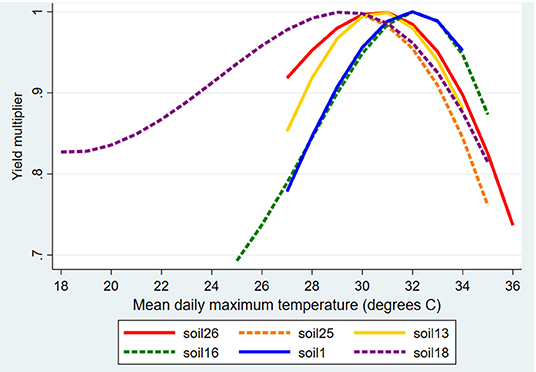
Figure 1. Relative yield benefits for high-yield rainfed maize on the six most common soil types in response to the mean daily maximum temperature of the second month, °C. Using a cubic specification for rainfall and mean daily maximum temperature, with log yield as the dependent variable. Each soil is mapped over the range from the 5th to 95th percentile for temperatures used in building the emulator.

We also see that for most soils, a less than ideal but still plausible temperature can lead to up to a 20% reduction in yield. Note that this is a reduction for temperature during a single month. If other months also have less than ideal temperatures, then the effect is multiplicative for the log specification and additive when yield is the dependent variable. Because crops have an optimal temperature at which maximum yields are obtained, it is difficult to have intuition about the effect of climate change on yields due to heterogeneity across locations and months of the growing season. Too cold and an increase in temperature increases yields;¹ too hot and an increase in temperature decreases yields. Near the peak, an increase in temperature might not change the yield. Countries with diverse climates will experience a wide range of yield effects from climate change and might experience all three types of effects.

Figure 2 shows yield responses to rainfall in the second month of the growing season for the six major soil types in the study area. Soils have different water holding capacities, so it is not surprising that optimal rainfall ranges from around 160 to 240 mm for this month. We see from the graphs that even 1-month droughts can have a profound effect on maize yield. For the soils in Figure 2, precipitation at around 20 mm in the month leads to around a 50–60% reduction in maize yield. This shows the value of supplemental irrigation in places where rainfall is unreliable. We also see from the graphs that too much rain can lead to a reduction in yield, though the affect varies across soil types.

FIGURE 2

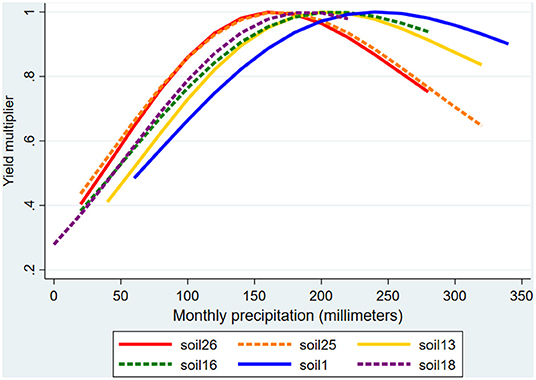
Figure 2. Relative yield benefits for high-yield rainfed maize on the six most common soil types in response to rainfall in the second month, millimeters. Using a cubic specification for rainfall and mean daily maximum temperature, with log yield as the dependent variable. Each soil is mapped over the range from the 5th to 95th percentile for temperatures used in building the emulator.

Though not reported here, we experimented with other explanatory variables such as interaction terms between temperature and precipitation and using cumulative seasonal rainfall in addition to monthly rainfall. While the R-squared improved slightly it took away from being able to have intuition in how the yield responds to different climate values, so we decided not to include them.

Figure 3 shows the yield responses to rainfall in the second month of the growing season for rainfed groundnuts on the six most common soils for the region. Unlike the maize response to rainfall in cubic specification, we do not note any sizable reduction in yield for high levels of rainfall for any of the soil types here.

FIGURE 3

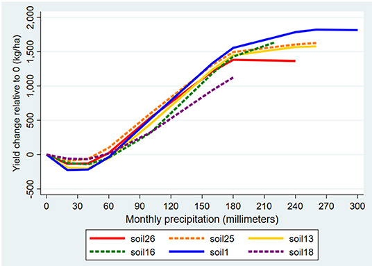
Figure 3. Relative yield benefits for rainfed groundnuts on the six most common soil types in response to rainfall in the second month, millimeters. Used a piecewise linear specification with seven segments for rainfall and the same for mean daily maximum temperature, with yield as the dependent variable. Each soil is mapped over the range from the 5th to 95th percentile for temperatures used in building the emulator. Yields are relative to the yield for no rainfall.

Results

Evaluating the Impact of Climate Change on Maize Yields

Future yields are predicted for the 455 Gaussian quadrature climates for each of the emissions scenarios and for all 50-years of the time period under study, using the regression parameters discussed in the previous section. The predictions are computed at each quarter-degree pixel and for each year from 2020 to 2069. In order to aggregate the yields to the country level, SPAM 2010 (You et al., 2014) is used to provide estimations of the number of hectares of each crop that are grown in each pixel. This allows us to compute total national production and total cultivated area, which by dividing production by area gives the appropriate measure of mean national yield for every year.

Figure 4 illustrates the distribution of maize yields for 3 different decades under the 4 different emissions scenarios, based on a representative selection of climates and weathers under those scenarios. 1.5C has the lowest greenhouse gas (GHG) emissions and represents the level that will keep average temperature change at 1.5°C; followed by 2C (keeping temperatures at 2°C); PF, based on keeping the Paris Agreement levels forever; and REF, which is unconstrained by international treaties (Schlosser et al., 2020, 2021). We note that the yield distributions change very little by the 2060s for the 1.5C and 2C scenarios—an important finding in itself, because it suggests that the region would be unaffected in the aggregate—though it would be at national and subnational levels—if global emissions can be capped at levels suggested by the IPCC and others. Yields decline noticeably in the PF scenario and even more so in the REF scenario, pointing to the fact that higher emissions have greater negative consequences for agricultural productivity for the region.

FIGURE 4

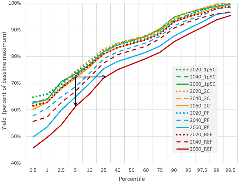
Figure 4. Modified distribution function of climate change on rainfed maize yields for the 10-country study area across decades and across emissions scenarios. Source: Authors.

In Figure 4 we also note that the consequences for higher emissions on maize yields are greater for the low-yield years than for the high-yield years. The importance of such a finding is that while yield loss in a typical year is something to be concerned about, yield loss in a bad-weather, low-yield year can lead to much greater consequences for food insecurity and hunger, not only for small-holder farmers relying on home production but by driving prices for staple foods higher, burdening both rural non-farm and urban households. If governments and donors fail to account for the much stronger climate impact on production in years with adverse weather, they could potentially under-invest in climate adaptation and resilience. Since almost all previous studies focus on the average impact, this is likely to have been the case thus far.

The depth of the impact can be measured in several ways, but the arrows in Figure 4 suggest two of them. First, we can look at the change in yields in the tail of the distribution. At the 5th percentile, for example, we see that the yield in the 2060s REF scenario is 13 percentage points lower than the baseline in the 2020s. That is, if typical (median) yield at the regional level is 2,000 kilograms per hectare, the baseline 5th percentile is about 73% of that, or around 1,450 kilograms per hectare. But in the 2060s PF scenario, it is another 11% points lower (226 kg/hect)—so the yield in a 1-in-20-year event would no longer be 1,450 kg/hect but 1,224 kg/hect. While the median in the 2060s REF is 91% of the baseline median, the 5th percentile in the 2060s REF is 84% of the baseline 5th percentile. This way of considering the costs of climate change during low-yield years is given by the vertical arrow in Figure 4, which shows change in yield for the 5th percentile from the 2020s to the 2060s.

A second way to consider the impact of the magnitude of changes in yields in the tail of the distribution is in the frequency of low-yield events. An event in the 5th percentile will occur on average every 20 years. That is, yields that low or lower occur 5% of the time, which means 5 out of 100 years, or equivalently, 1 out of 20 years. We can ask how frequently today's low-yield, 20-year event will occur in the future under climate change. Under the REF scenario in the 2060s, we can see that a 20-year event in the baseline will occur every 3.5 years in the 2060s, as illustrated by the horizontal line in Figure 4.

Thus far, we have considered the aggregated impact on yields for the region. However, effects on individual localities must be considered as the climate varies across the region, and climate change will affect the region differently across locations. Since our analysis is done at a pixel level (quarter-degree or roughly 25 km), we can aggregate the results to any level we choose. In Figure 5, we compare the change in yield distributions in each of the 10 countries. Focusing on the high-emissions REF scenario, we find that for almost all of the countries, low-yield years will experience greater relative yield losses than typical years—just as we saw for the regional aggregate.

FIGURE 5

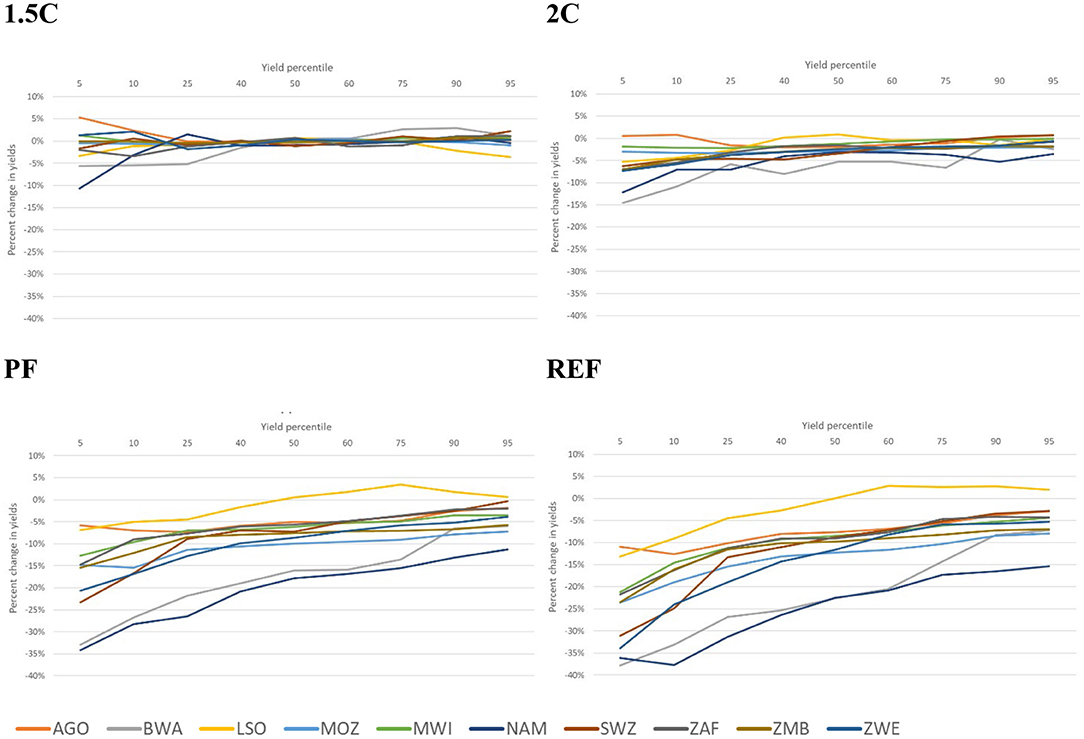
Figure 5. Impact of climate change on change in rainfed maize yields by country and percentile, 2020s to 2060s. Source: Authors.

This rule does not hold for Angola for the REF scenario, as the left tail of the distribution does not drop off rapidly, but in fact rises higher in the 1st percentile (not pictured). Meanwhile, the left tail is higher at the 5th percentile than at the median in the other emissions scenarios. This shows that we cannot assume what will happen with the relative impact of climate change for low-yield vs. median-yield years. We also see in the REF scenario that Botswana, Namibia, Eswatini and Zimbabwe exhibit more of a negative response during low-yield years than what the regional aggregate showed.

With diminished emissions we note much smaller impact on yields across all percentiles of the distribution—an important and not well-accounted benefit of reducing emissions. Nonetheless, even in the lowest emissions scenario, 1.5C, we see that there is often a much larger yield effect during years experiencing low-yield events compared to normal years.

Table 2 displays median yield changes by country and for the region. In the highest emissions scenario, median yields will decline by 9.2% by the 2060s due to climate change, but only 3.1% by the 2040s. The decline is smaller in the PF scenario, and virtually no change in the two lowest emissions scenarios. The table shows that not all countries will be impacted evenly, as the REF scenario projects that by the 2060s, Botswana and Namibia will have the highest losses for the region, followed by Mozambique and Zimbabwe.

TABLE 2

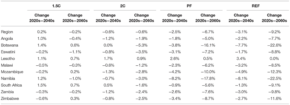
Table 2. Change in median yield for rainfed maize under climate change for 4 emissions scenarios from 2020s in 2040s and 2060s.

Since we have noted a heterogeneous effect across the region at the national level, we would expect that there would also be a heterogeneous impact of climate change within countries. Figure 6 presents the percentage point difference between the 50th and 5th percentiles, representing the relative impact of climate change on low-yield years compared to typical years.

FIGURE 6

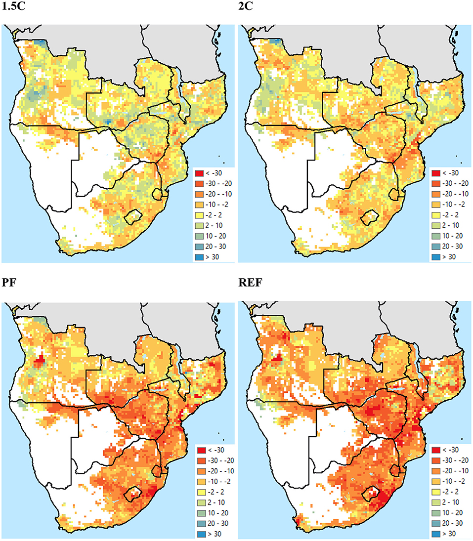
Figure 6. Percentage point difference between change in yield of rainfed maize from baseline for the 50th percentile and change for the 5th percentile, REF scenario, 2020s to 2060s. Source: Authors. The map shows only areas that grow rainfed maize.

In the high-emissions REF scenario, much of the northern part of the region, which tends to have higher rainfall than the southern portion exhibits only a small difference between yield change at the 50th percentile and yield change at the 5th percentile. Some sites had fewer losses at the 5th percentile. However, other regions within countries have much higher losses in the bad-weather, low-yield years, such as those along the northeast coast of South Africa.

Some areas—including large portions of Angola, South Africa, and Zimbabwe—exhibit greater yield losses (smaller yield gains) at the medians than at the 5th percentile in the lower emissions scenarios. The same areas exhibit smaller yield losses in the higher emissions scenario.

Schlenker and Roberts (2009), using historical yield data at the national level estimate regression models linking yields to temperature and precipitation. Using 16 older AR4 GCMs and a single emissions scenario, they project the impact on maize yields on several African countries, including 4 in our study area. They predict very large yield losses, particularly for Zambia (around 38%) and South Africa (around 30%), and lower for Malawi and Mozambique (around 18% for each). They also project uncertainty based on variation across climate models and uncertainty in their parameter estimates. This differs from what we did here, because our sources of uncertainty include inter-annual variation in climate and uncertainty over the future emissions.

As mentioned, after analyzing the changes in yields in the tail of the distribution, we consider the frequency of low-yield events. Table 3 shows how often the yield of a 20-year event in the 2020s will occur in the 2040s and in the 2060s. At the regional level under the REF emissions scenario, the 20-year event occurs roughly twice as often by the 2040s but nearly six times as often by the 2060s. Many of the countries only indicate a modest shift by the 2040s, but by the 2060s, the frequency largely increases in each country except Lesotho, which experiences a relatively small doubling in frequency compared to the 2020s.

TABLE 3

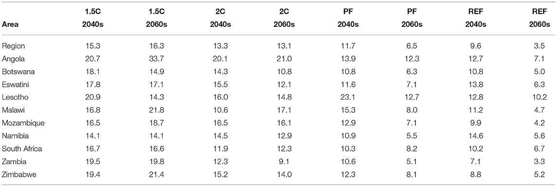
Table 3. Frequency of 20-year low-yield events for rainfed maize from 2020s in 2040s and 2060s, REF scenario.

The PF and REF scenarios both exhibit an increase in frequency of extreme events from the 2020s to the 2040s and again from the 2040s to the 2060s. For both the 1.5C and 2C scenarios, the frequency of low-yield events generally stops increasing after the 2040s, and the level in the 2040s is much less than in either the PF or REF scenarios. In Angola, the frequency of low-yield events in the 2060s in is less than the frequency in the 2020s. The negative effects of climate change appear to stop and even reverse in the 1.5C scenario, at least in some countries.

Figure 7 shows the spatial heterogeneity that informs the national level data in Table 3. Not surprisingly, however, it is similar in appearance to Figure 6. The bright red regions in the REF scenario are projected to have four times the number of low-yield events in the 2060s. These maps could potentially help planners identify areas to target for interventions to reduce risk for farmers. Every country includes a number of regions in which low-yield events actually decline by the 2060s in the 1p5C scenario.

FIGURE 7

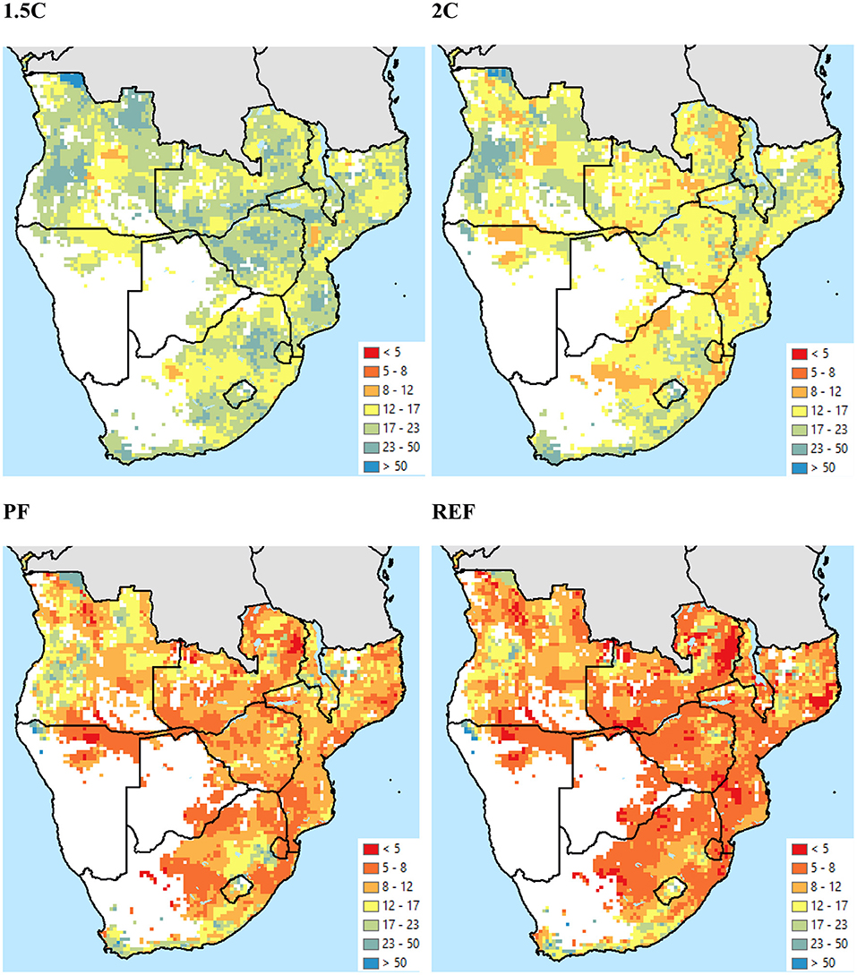
Figure 7. New frequency of 20-year low-yield events for rainfed maize in 2060s under REF relative to 2020s REF. Source: Authors.

Evaluating the Impact of Climate Change on Drybean Yields

Importance for the Countries of the Region

Drybeans represent an important source of plant protein for the region, with almost all of the production staying within each country for food as well as seed supply (FAO et al., 2020). For four of the ten countries in the region, drybeans represent the third most important crop in terms of area cultivated, as they do for the region as a whole. According to FAOSTAT (FAO, 2020) however, they do not appear to be very important for production in Namibia, Botswana, and Zambia (the latter two do not seem to produce any), and are of only modest importance in South Africa, Zimbabwe, and Eswatini. Angola is the largest producer in the region, with almost half the cultivated area and 40% of the production. The highest yields are produced by Namibia (which has <0.01% of the region's total area for drybean cultivation) and South Africa.

Yield Changes

In generating yields for the emulator using DSSAT, we used four varieties of drybean that were appropriate for the region, and selected the highest yielding variety among the four at each pixel, year, and climate. The projected impact of climate change on rainfed drybean production is shown in Table 4, which focuses in on only two of the four emissions scenarios, 2C and PF. Under the low emissions scenario (2C), most countries for which drybean production is important experience very little yield reduction even through the 2060s. However, under the higher emissions scenario, Angola is projected to have a nearly 7% yield reduction by the 2060s, followed by Mozambique and Malawi, with losses under 6%. Lesotho's drybean production, on the other hand, will not be affected much at all by climate change. The largest losses will be seen in Namibia and Zimbabwe, for which drybean production is not of great importance.

TABLE 4

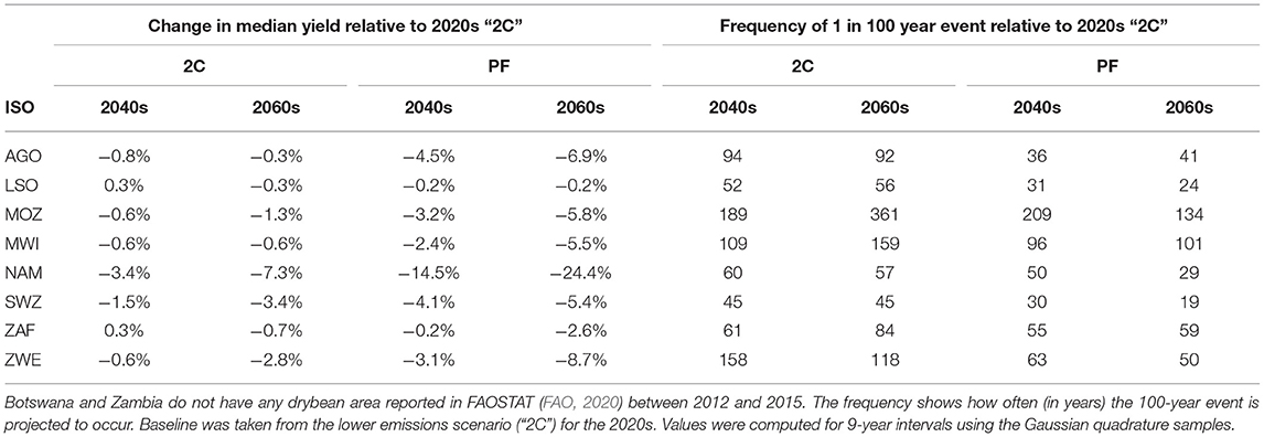
Table 4. Changes in median yields and frequency of catastrophic yields for rainfed drybeans under climate change.

The frequency of 1-in-100 year low-yield events, however, will have a greater effect on Eswatini, for which they will occur 5 times as often, and Lesotho, for which they will occur 4 times as often. Even Angola will see a much great frequency, with those extreme events occurring 2.5 times as often.

Evaluating the Impact of Climate Change on Groundnut Yields

Importance for the Countries of the Region

Groundnuts are the fourth most important crop for the region as measured by area cultivated. It is the second most important crop for both Malawi and Zambia, however, representing 9.0 and 9.6% of cultivated area. It is also of high importance to Angola, Mozambique, and Zimbabwe, ranking fourth or fifth among all crops for each country, and 6.7% of cultivated area or above.

Yield Changes

Table 5 shows the impact of climate change on groundnuts. We generated yields in DSSAT for two groundnut varieties that were appropriate for the region, and selected the highest yielding variety of the two at each pixel, year, and climate. Of the crops for which groundnuts are of high importance, Zimbabwe shows the greatest potential climate impact. At the lower emissions scenario, even by the 2060s, yield reductions should only be around 3%, but at the higher emissions level, losses should be over 6% by the 2040s and over 10% by the 2060s. South Africa, which has only 1% of area in groundnuts, could experience 20% yield reduction by the 2060s compared to production in the 2020s.

TABLE 5

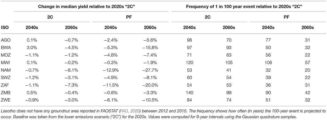
Table 5. Changes in median yields and frequency of catastrophic yields for rainfed groundnuts under climate change.

On the positive side, Malawi, which is the region's leading producer and second highest with groundnut area cultivated, should have yield only slightly affected by climate change, with reductions even by the 2060s under the high emissions scenario at <2%.

However, in terms of extreme low-yield events, Mozambique, which has the region's highest amount of area in groundnut cultivation should see events occur almost 5 times more frequently, and Angola, Zimbabwe, and South Africa should see them occur 3 times more frequently.

Evaluating the Impact of Climate Change on Soybean Yields

Importance for the Countries of the Region

Soybeans are the sixth most important crop for the region, but this is driven in large part by South Africa, for which soybeans are the second most important crop in terms of cultivated area. South Africa produces almost 70% of the region's soybeans and has just under 64% of the region's soybean area. Soybeans also appear to be of moderate importance to Zambia and to a lesser extent to Malawi and Zimbabwe. According to FAOSTAT (FAO, 2020), five of the region's ten countries do not grow any soybeans.

Yield Changes

Table 6 tells us that the region's largest soybean producer, South Africa, will experience virtually no yield impact from climate change. Because the computation is done at the pixel level and the pixels are weighted by the modeled cultivated area inside them, it is difficult to know precisely why the high emissions scenario shows less yield reduction in the 2060s than in the 2040s, and less than the low emissions scenario in the 2060s. But it may simply be that soybeans are cultivated in areas in which the current temperature is slightly sub-optimal, and additional warming take it past optimal, but not very far past.

TABLE 6

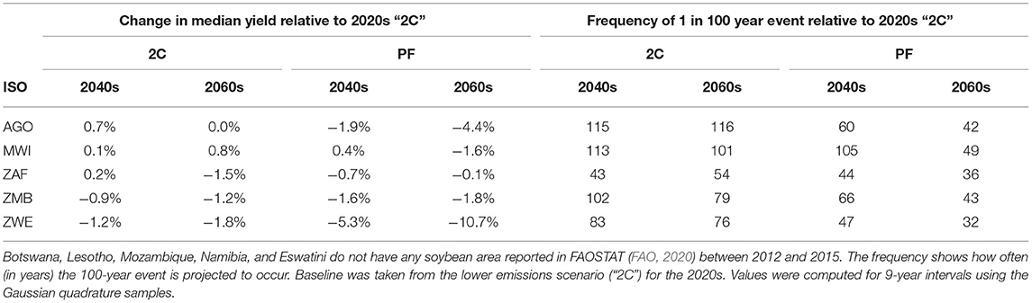
Table 6. Changes in median yields and frequency of catastrophic yields for rainfed soybeans under climate change.

Zimbabwe is projected to experience the largest losses for soybeans from climate change at almost 11% in the 2060s under the higher emissions scenario, though it only represents around 2% of total cultivated area for the country. Nonetheless, we see that under the lower emissions scenario, yield reductions will be much less.

For all of the countries in the study area—including South Africa—by the 2060s under the higher emissions scenario, the frequency of extreme low-yield events will at least double and perhaps triple in frequency. Strangely, this is true in South Africa across all decades and emissions scenarios, reflecting that the worst effect of climate change on soybean yields will be experienced by the 2040s. However, for some of the other countries, lower emissions reduce the frequency of extreme low-yield events.

Discussion

We have carefully analyzed the impact of climate change on yields of four key crops for Southern Africa. Our analysis considered not just the median impacts but the effects on extreme events—years with very low yields due to adverse weather. The analysis was done at a very fine spatial resolution with the results aggregated to each of the ten countries in the region. We saw not only how climate change will impact agriculture in typical years, but how in bad years the impact on agriculture in most cases will be greater.

We focused most on maize, which is an invaluable commodity for the region as the leading source of both calories and protein for consumers in the 10 countries of Southern Africa while occupying 41% of the region's cultivated area. Maize provides the main source of nutrition for some of the most food insecure people of the region. Investigating how a changing climate will affect maize production in low-yield years has revealed that if emission levels are high, the low-yield, 1-in-20-year events for the region produce 16% lower yields in the 2060s than in the 2020s, while at the median year, the yields will be 9% lower. Furthermore, the frequency at which the 1-in-20-year low-yield event occurs will decrease to 1-in-3.5-year events.

Averaging across a large area tends to hide losses that can be locally high. Examining the impact of climate change on the cropping sector for countries of the region, Botswana could be the country hit the hardest among the 10 in the study area, because of the importance of maize to farmers and because of the severity of the impact of climate change on maize yield.

On the other hand, Lesotho appears to benefit from climate change at the median of the projections, though very little. However, the change in frequency of extreme low-yield events could adversely impact even countries like Lesotho, with the frequency of low-yield events increasing to 3 or 4 times the rate that they are currently occurring.

This study on the impact of climate change, uncertainty, and inter-annual variability on agricultural production is also essentially one dealing with issues of food insecurity under climate change. Except for soybeans, the crops examined in this study are ones that are produced and consumed by subsistence farmers, so that increasing the frequency of low-yield events is also a threat to food security which in many countries is a much bigger problem in rural areas than urban.

This kind of analysis is immensely useful for both the public and private sector in evaluating the benefits of longer-term investments designed to support agriculture and nutrition. The long-term costs of low yields can be significant, between loss of life; child malnutrition, which can lead to reduction in lifetime earning potential; and loss of capital and livestock (if households sell items to compensate for food shortages). As costs of losses in low-yield years are higher than costs in median years, it is likely that governments and businesses have under-estimated the full cost of climate change and have therefore under-invested in things such as irrigation, insurance (crop and weather), agricultural research and extension, and capacity for delivering social protection, all of which—if sufficiently invested in—could reduce the losses during bad-weather years.

This analysis could assist in optimally targeting interventions sub-nationally, since our findings show that the effect of climate change is spatially heterogeneous, with some parts of countries facing much larger losses than others. Focusing on the areas that will be hit the hardest could potentially give more return to investment in impact mitigation strategies. Interventions could include introducing new crops—such as millet in place of sorghum or maize—in areas that are likely to be most affected by climate change hardest hit.

Finally, while we have used the large climate ensemble to examine low-yield agricultural events, the data and methodology could be applied to a wider range of climate impacts including the effects on livestock, human labor, hydrology, energy, and infrastructure.

Data Availability Statement

The raw data supporting the conclusions of this article will be made available by the authors, without undue reservation.

Author Contributions

TT was the lead writer of this paper and generated weathers for DSSAT, built the emulators, and generated the final yield output used. RR produced the DSSAT results and advised on the emulator, as well as helped in editing. KS provided overall guidance and particularly supported irrigation inputs for crop production. CA served as principal investigator of the project and wrote the basic Gaussian quadrature program, assisted on its application to this project, and helped in editing. All authors contributed to the article and approved the submitted version.

Funding

We are grateful for support from the CGIAR Research Program on Policies, Institutions, and Markets (PIM); the CGIAR Research Program on Water, Land and Ecosystems (WLE); the One CGIAR Initiative on Foresight and Metrics to Accelerate Food, Land, and Water Systems Transformation; and the National Treasury, Republic of South Africa.

Conflict of Interest

The authors declare that the research was conducted in the absence of any commercial or financial relationships that could be construed as a potential conflict of interest.

Publisher's Note

All claims expressed in this article are solely those of the authors and do not necessarily represent those of their affiliated organizations, or those of the publisher, the editors and the reviewers. Any product that may be evaluated in this article, or claim that may be made by its manufacturer, is not guaranteed or endorsed by the publisher.

Acknowledgments

The authors would like to thank Meschelle Thatcher who lent support to the team through finding background material and reviewing the content of the article.

Footnotes

1. ^Parts of Southern Africa can experience cold weather, since it extends below 34 degrees South and also has several peaks above 3,400 meters elevation.

References

Arndt, C., Fant, C., Robinson, S., and Strzepek, K. (2015). Informed selection of future climates. Clim. Change 130, 21–33. doi: 10.1007/s10584-014-1159-3

CrossRef Full Text | Google Scholar

Bathiany, S., Dakos, V., Scheffer, M., and Lenton, T. M. (2018). Climate models predict increasing temperature variability in poor countries. Sci. Adv. 4, eaar5809. doi: 10.1126/sciadv.aar5809

PubMed Abstract | CrossRef Full Text | Google Scholar

Blanc, E., and Sultan, B. (2015). Emulating maize yields from global gridded crop models using statistical estimates. Agric. Forest Meteorol. 214–215, 134–147. doi: 10.1016/j.agrformet.2015.08.256

CrossRef Full Text | Google Scholar

Burke, M., Dykema, J., Lobell, D. B., Miguel, E., and Satyanath, S. (2015). Incorporating climate uncertainty into estimates of climate change impacts. Rev. Econ. Stat. 97, 461–471. doi: 10.1162/REST_a_00478

PubMed Abstract | CrossRef Full Text | Google Scholar

Chen, Y., Zhang, Z., and Tao, F. (2018). Impacts of climate change and climate extremes on major crops productivity in china at a global warming of 1.5 and 2.0°C. Earth Syst. Dynam. 9, 543–562. doi: 10.5194/esd-9-543-2018

CrossRef Full Text | Google Scholar

Dell, M., Jones, B. F., and Olken, B. A. (2014). What do we learn from the weather? The new climate-economy literature. J. Econ. Liter. 52, 740–798. doi: 10.1257/jel.52.3.740

CrossRef Full Text | Google Scholar

FAO (2020). FAOSTAT Database. Rome: FAO. Downloaded January 21, 2021.

FAO IFAD, UNICEF, WFP, and WHO. (2018). The State of Food Security and Nutrition in the World 2018. Building Climate Resilience for Food Security and Nutrition. Rome: FAO.

FAO IFAD, UNICEF, WFP, and WHO. (2020). The State of Food Security and Nutrition in the World 2020. Transforming Food Systems for Affordable Healthy Diets. Rome: FAO.

Franke, J. A., Müller, C., Elliott, J., Ruane, A. C., Jägermeyr, J., Snyder, A., et al. (2020). The GGCMI Phase 2 emulators: global gridded crop model responses to changes in CO2, temperature, water, and nitrogen (version 1.0). Geosci. Model Dev. 13, 3995–4018. doi: 10.5194/gmd-13-3995-2020

CrossRef Full Text | Google Scholar

Gaupp, F., Hall, J., Hochrainer-Stigler, S., and Dadson, S. (2020). Changing risks of simultaneous global breadbasket failure. Nat. Clim. Chang. 10, 54–57. doi: 10.1038/s41558-019-0600-z

CrossRef Full Text | Google Scholar

Jägermeyr, J., Müller, C., Ruane, A. C., Elliott, J., Balkovic, J., Castillo, O., et al. (2021). Climate impacts on global agriculture emerge earlier in new generation of climate and crop models. Nat. Food 2, 873–885. doi: 10.1038/s43016-021-00400-y

CrossRef Full Text | Google Scholar

Jones, J. W., Hoogenboom, G., Porter, C. H., Boote, K. J., Batchelor, W. D., Hunt, L. A., et al. (2003). The DSSAT cropping system model. Eur. J. Agron. 18, 235–265. doi: 10.1016/S1161-0301(02)00107-7

CrossRef Full Text | Google Scholar

Koo, J., and Dimes, J. (2010). HC27 Soil Profile Database. Washington, DC: International Food Policy Research Institute. Available online at: http://hdl.handle.net/1902.1/20299

Liu, W., Ye, T., and Shi, P. (2021). Decreasing wheat yield stability on the North China plain: relative contributions from climate change in mean and variability. Int. J. Climatol. 41, E2820–E2833. doi: 10.1002/joc.6882

CrossRef Full Text | Google Scholar

Lobell, D. B., Schlenker, W., and Costa-Roberts, J. (2011). Climate trends and global crop production since 1980. Science 333, 616–620. doi: 10.1126/science.1204531

PubMed Abstract | CrossRef Full Text | Google Scholar

Miao, R., Khanna, M., and Huang, H. (2015). Responsiveness of crop yield and acreage to prices and climate. Am. J. Agric. Econ. 98, 191–211. doi: 10.1093/ajae/aav025

CrossRef Full Text | Google Scholar

Müller, C., and Robertson, R. (2014). Projecting future crop productivity for global economic modeling. Agric. Econ. 45, 37–50. doi: 10.1111/agec.12088

CrossRef Full Text | Google Scholar

Ostberg, S., Schewe, J., Childers, K., and Frieler, K. (2018). Changes in crop yields and their variability at different levels of global warming. Earth Syst. Dynam. 9, 479–496. doi: 10.5194/esd-9-479-2018

CrossRef Full Text | Google Scholar

Pendergrass, A. G., Knutti, R., Lehner, F., Deser, C., and Sanderson, B. M. (2017). Precipitation variability increases in a warmer climate. Sci. Rep. 7, 17966. doi: 10.1038/s41598-017-17966-y

PubMed Abstract | CrossRef Full Text | Google Scholar

Reilly, J., Chen, Y. H., Sokolov, A., Gao, X., Schlosser, A., Morris, J., et al. (2018). Food, Water, Energy, Climate Outlook, 2018, MIT Joint Program on the Science and Policy of Global Change. Available online at: https://globalchange.mit.edu/outlook2018 (accessed July 2, 2020).

Rosenzweig, C., Elliott, J., Deryng, D., Ruane, A., Müller, C., Arneth, A., et al. (2014). Assessing agricultural risks of climate change in the 21st century in a global gridded crop model intercomparison. PNAS. 111, 3268–3273. doi: 10.1073/pnas.1222463110

PubMed Abstract | CrossRef Full Text | Google Scholar

Schlenker, W., and Roberts, M. J. (2009). Nonlinear temperature effects indicate severe damages to u.s. crop yields under climate change. Proc. Natl. Acad. Sci. U. S. A. 106, 15594–15598. doi: 10.1073/pnas.0906865106

PubMed Abstract | CrossRef Full Text | Google Scholar

Schlosser, C. A., Gao, X., Strzepek, K., Sokolov, A., Forest, C. E., Awadalla, S., et al. (2012). Quantifying the likelihood of regional climate change: a hybridized approach. J. Clim. 26, 3394–3414. doi: 10.1175/JCLI-D-11-00730.1

CrossRef Full Text | Google Scholar

Schlosser, C. A., Sokolov, A., Strzepek, K., Thomas, T., Gao, X., and Arndt, C. (2020). The Changing Nature of Hydroclimatic Risks Across South Africa. Joint Program Report Series Report 342. Available online at: http://globalchange.mit.edu/publication/17483 (accessed September 29, 2020).

Schlosser, C. A., Sokolov, A., Strzepek, K., Thomas, T., Gao, X., and Arndt, C. (2021). The changing nature of hydroclimatic risks across South Africa. Clim. Change 168, 1–25. doi: 10.1007/s10584-021-03235-5

CrossRef Full Text | Google Scholar

Sheffield, J., Goteti, G., and Wood, E. F. (2006). Development of a 50-yr high-resolution global dataset of meteorological forcings for land surface modeling. J. Clim. 19, 3088–3111. doi: 10.1175/JCLI3790.1

CrossRef Full Text | Google Scholar

Sokolov, A., Kicklighter, D., Schlosser, A., Wang, C., Monier, E., Brown-Steiner, B., et al. (2018). Description and evaluation of the MIT Earth System Model (MESM). J. Adv. Model. Earth. Syst. 10, 1759–1789. doi: 10.1002/2018MS001277

CrossRef Full Text | Google Scholar

Stuch, B., Alcamo, J., and Schaldach, R. (2020). Projected climate change impacts on mean and year-to-year variability of yield of key smallholder crops in sub-Saharan Africa. Clim. Dev. 13, 268–82 doi: 10.1080/17565529.2020.1760771

CrossRef Full Text | Google Scholar

Thomas, T. (2015). US Maize Data Reveals Adaptation to Heat and Water Stress: IFPRI Discussion Paper 01485 (December). Washington, DC: IFPRI. Available online at: http://www.ifpri.org/cdmref/p15738coll2/id/129841/filename/130052.pdf

Thomas, T. S., Schlosser, C. A., Strzepek, K., Robertson, R. D., and Arndt, C. (2022). Using a large climate ensemble to assess the frequency and intensity of future extreme climate events in Southern Africa. Front. Clim. 4, 787721. doi: 10.3389/fclim.2022.787721

CrossRef Full Text | Google Scholar

Thome, K., Meade, B., Daugherty, K., and Christensen, C. (2018). International Food Security Assessment, 2018-2028, GFA-29, U.S. Department of Agriculture, Economic Research Service, June.

Thornton, P., Jones, P., Alagarswamy, G., and Andresen, J. (2009). Spatial variation of crop yield response to climate change in East Africa. Glob. Environ. Chang. 19, 54–65. doi: 10.1016/j.gloenvcha.2008.08.005

CrossRef Full Text | Google Scholar

Torriani, D. S., Calanca, P., Schmid, S., Beniston, M., and Fuhrer, J. (2007). Potential effects of changes in mean climate and climate variability on the yield of winter and spring crops in Switzerland. Clim. Res. 34, 59–69. doi: 10.3354/cr034059

CrossRef Full Text | Google Scholar

United Nations (2015). Transforming Our World: The 2030 Agenda For Sustainable Development. Available online at: https://sdgs.un.org/sites/default/files/publications/21252030%20Agenda%20for%20Sustainable%20Development%20web.pdf

van der Wiel, K., and Bintanja, R. (2021). Contribution of climatic changes in mean and variability to monthly temperature and precipitation extremes. Commun. Earth Environ. 2, 1. doi: 10.1038/s43247-020-00077-4

CrossRef Full Text | Google Scholar

You, L., Wood, S., Wood-Sichra, U., and Wu, W. (2014). Generating global crop distribution maps: from census to grid. Agric. Syst. 127, 53–60. doi: 10.1016/j.agsy.2014.01.002

CrossRef Full Text | Google Scholar

Zabel, F., Müller, C., Elliott, J., Minoli, S., Jägermeyr, J., Schneider, J. M., et al. (2021). Large potential for crop production adaptation depends on available future varieties. Glob. Change Biol. 27, 3870–3882. doi: 10.1111/gcb.15649

PubMed Abstract | CrossRef Full Text | Google Scholar