 Hamish D. Pritchard
94% of researchers rate our articles as excellent or good
Learn more about the work of our research integrity team to safeguard the quality of each article we publish.
Find out more
PERSPECTIVE article
Front. Clim., 14 June 2021
Sec. Predictions and Projections
Volume 3 - 2021 | https://doi.org/10.3389/fclim.2021.689823
This article is part of the Research TopicKnowledge Gaps from the IPCC Special Report on the Ocean and Cryosphere in a Changing Climate and Recent AdvancesView all 14 articles
The IPCC Special Report on Oceans and Cryosphere in a Changing Climate identified major gaps in our knowledge of snow and glacier ice in the terrestrial cryosphere. These gaps are limiting our ability to predict the future of the energy and water balance of the Earth's surface, which in turn affect regional climate, biodiversity and biomass, the freezing and thawing of permafrost, the seasonal supply of water for one sixth of the global population, the rate of global sea level rise and the risk of riverine and coastal flooding. Snow and ice are highly susceptible to climate change but although their spatial extents are routinely monitored, the fundamental property of their water content is remarkably poorly observed. Specifically, there is a profound lack of basic but problematic observations of the amount of water supplied by snowfall and of the volume of water stored in glaciers. As a result, the climatological precipitation of the mountain cryosphere is, for example, biassed low by 50–100%, and biases in the volume of glacier ice are unknown but are likely to be large. More and better basic observations of snow and ice water content are urgently needed to constrain climate models of the cryosphere, and this requires a transformation in the capabilities of snow-monitoring and glacier-surveying instruments. I describe new solutions to this long-standing problem that if deployed widely could achieve this transformation.
The IPCC Special Report on Oceans and Cryosphere in a Changing Climate (SROCC) highlighted key strengths and weaknesses in our understanding of the cryosphere (IPCC, 2019). It showed that we can observe with high or very high confidence (IPCC confidence definitions in italics) loss of mass from the ice sheets (SROCC section A.1.1), declining sea ice (SROCC A.1.4), and snow cover (SROCC A.1.2), and can produce probabilistic climate projections across a range of future scenarios. For many aspects of the cryosphere, however, it is only the trajectories of change that can be projected with medium to very high confidence. Their magnitudes are either not quantified, have large uncertainties or are quantified with low confidence. These include terrestrial snow cover (SROCC A.1, A.7.7, A.4.1, A.1.4, A.1.2, B.1.3), mountain and Arctic water resources (SROCC A.7.6, B.1.6, B.7, B.4.3), permafrost thaw (SROCC B.7.2), mountain and polar species distribution, biodiversity and biomass (SROCC B.4, B.4.1, B.4.2) and disaster risk (SROCC B.1.5, B.7.1).
Major deficiencies in snow and ice observations from mountain ranges and the Polar Regions contribute to this uncertainty. “Clear knowledge gaps” exist in current glacier-ice volumes and the spatial and temporal variation of snow cover (SROCC section 2.5). Time-series of snow water equivalent (SWE) show “reasonable consistency” when averaged by continent but considerable disagreement in spatial pattern (SROCC section 3.4). Knowledge of SWE trends is “inadequate” (SROCC section 3.7), and mountain precipitation trends globally are “highly uncertain” due to large natural variability and “intrinsic uncertainties” in measurements (SROCC section 2.5). Long-term observations are particularly scarce in High Mountain Asia (HMA), Northern Asia and South America (SROCC section 2.2.2). Similarly over Arctic land, precipitation measurements are “sparse and highly uncertain” (SROCC section 3.7). Atmospheric re-analyses suggest a recent Arctic-precipitation increase but the wide model spread gives only low confidence in reanalysis-based closure of the Arctic freshwater budget. A declining trend in snow-depth in the Russian Arctic was assigned medium confidence as the “pointwise nature” of weather-station measurements does not capture prevailing conditions across the landscape. A shift in the timing of maximum snow depth was detected for the North American Arctic but no comparable analysis is available for Eurasia (SROCC section 3.7).
Snow and ice strongly modify the albedo and insulation of land and sea surfaces, the wetting or drying (and greening or browning) of the terrestrial Arctic, and the mass balance of all of the world's glaciers and ice sheets. These weaknesses therefore critically impact our understanding of cold-region water and energy balances, with global consequences. Over the recent past, global glacier mass loss was as great as that from the Greenland Ice Sheet (the single largest source of sea level rise), but with 10-fold greater uncertainty (Figure 1). Due to the limited number of well-observed glaciers, there is only medium confidence in the ability of glacier models to reconstruct past sea-level change (SROCC section 4.2.2.2.3). Climate models also fail to reproduce a pre-1970 Greenland warming and resulting sea-level rise, hence there is only medium confidence in the ability of these models to predict future glacier and ice sheet surface mass balance (SMB) (SROCC section 4.2.2.6). These issues are reflected in projected future glacier losses under RCP2.6 by end-of-century that have a “likely” range of uncertainty of ±40%, using models calibrated with only “limited observations” and “diverging initial glacier volumes” (IPCC, 2019, CCB.6).
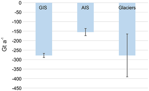
Figure 1. Annual rates of ice loss for 2006–2015 from the Greenland Ice Sheet (GIS) and Antarctic Ice Sheet (AIS) (IPCC, 2019, Table 3.3) and all other global glaciers (IPCC, 2019, section 2.2.3, Table 2.A.1). The glacier losses are as great as Greenland's but with much greater uncertainty.
Snowfall seasonally covers a third of all land (NSIDC, 2020) and exceeds 3000 Gt of transient water storage (Pulliainen et al., 2020) but snowfall SWE remains difficult to measure, particularly over mountains and the Polar Regions. Globally, most observations come from weather stations such as those contributing to the Global Historical Climate Network (GHCN), a quality-controlled database of 100,000 daily measurements (Menne et al., 2012) of which 26% report precipitation in the cryosphere and only 6% in the mountain cryosphere (Figure 2A). Only a single active GHCN station on the dry Tibetan Plateau reports daily precipitation in the combined 566,000 km2 Himalayan headwaters of the Brahmaputra, Indus and Ganges river basins above 4,000 m altitude (Figure 2A). Furthermore, the number of weather stations has decreased and is now at its lowest in over 100 years (Fick and Hijmans, 2017).
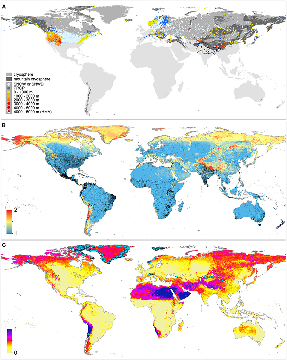
Figure 2. (A) Weather stations (coloured dots) in the Global Historical Climate Network that lie within the terrestrial cryosphere (mid grey), or more specifically within the mountain cryosphere (dark grey) and whose daily observations are ongoing (in 2020/21). Light blue dots show stations in the lowland terrestrial cryosphere that report either snowfall water content (SNOW) or depth (SNWD). Dark blue dots show stations that reported precipitation (PRCP) but do not distinguish snow observations. Yellow to red dots show stations within the mountain cryosphere that report SNOW or SNWD, coloured according to altitude. Black polygons show the river basins of the Indus (I), Ganges (G), and Brahmaputra (B). The cryosphere is defined as having a mean monthly temperature <0°C in January and/or July. The mountain cryosphere is the intersection between these areas and mountain areas (Karagulle et al., 2017). This highlights the paucity of snow observations in much of the mountain and Arctic cryosphere. (B) Bias-correction factors (blue-to-red scale, after Beck et al., 2020) that must be applied to the observation-based “WorldClim v2” annual climatological precipitation product (Fick and Hijmans, 2017) in order to agree with observations and models of catchment hydrology. All WorldClim v2 weather stations that reported precipitation (RAINID) in the 1970–2000 period are shown by black dots. (C) The uncertainty range in the estimated bias correction factors in 2b (the upper bound of the factor minus the lower bound) (after Beck et al., 2020), and glaciers with a reported average thickness only (white dots) or thickness-profile data (blue dots) (GlaThiDa Consortium, 2020, accessed February 2021).
These observations do not adequately represent even the climatological-average precipitation in these environments. Gridded precipitation climatologies interpolated from GHCN station data [e.g., the “WorldClim v2” 1970–2000 mean (Fick and Hijmans, 2017)] correlate reasonably well (0.86) on the global scale with test data but universally less well in mountain ranges. More significantly, they systematically underestimate precipitation in much of the cryosphere by 50–100% (Figure 2B). WorldClim v2 precipitation in the cryosphere requires an average bias-correction factor (inferred from streamflow data) of 1.52 vs. 1.05 for the rest of the world (Beck et al., 2020). In the mountain cryosphere the global average bias-correction factor is 1.46 for annual precipitation, and 1.61 in winter. Regionally the factor is 1.55 annually in the HMA (1.90 in winter and 1.44 in summer), 1.5–2 annually throughout the Arctic, and up to 2.05 for the Andes in winter (Figure 2B). Such biases among mountains are also present in comparable gridded precipitation products produced by various methods, including PREC/L (Chen et al., 2002), CHELSA V1.2, CHPclim V1, GPCC V2015, GPCP V2.3, and MERRA-2 (Beck et al., 2020), and regional hydrological assessments (e.g., Wortmann et al., 2018; Pritchard, 2019). Although these bias corrections have been calculated, they apply only to climatological averages and not the daily timescales of weather models, and also have considerable uncertainty due to the challenges involved in calibrating precipitation from streamflow: the range in possible correction factors in the Andes locally exceeds 4.00 (Figure 2C).
In part these precipitation biases (that are worst in winter and in mountains) reflect a spatial-sampling problem in the cryosphere, but they also reflect a problem of inherent measurement bias. Mountain precipitation, and particularly snowfall, is relatively heterogeneous (Gerber et al., 2018) and so is often not well-sampled regionally by the cryosphere's sparse station network or locally by the very small physical size of pluviometers (<0.3 m diameter) relative to local snowfall variability or to the kilometre-scale grid cells of precipitation products (e.g., Dozier et al., 2016; McCrary et al., 2017; Sturm et al., 2017; Yao et al., 2018; Haberkorn, 2019; Yoon et al., 2019). Snowpack SWE was found to have a standard deviation of 21% within a plot of only 20 × 8 m, for example (Haberkorn, 2019). These sampling problems on the large and small scale are compounded by the characteristic snow “undercatch” of pluviometers that leads to a precipitation low-bias of up to 90% in windy conditions (e.g., Burgess et al., 2010; Beck et al., 2020).
Pluviometer undercatch can be partially mitigated by fences and baffles, but these are rarely in operational use (Yang, 2014). Other daily operational measurements of snowpack SWE (e.g., snow pillows, scales) or SWE proxies (e.g., sonic rangers, radiometers) also observe only small areas (Dozier et al., 2016), and scaling up from the snow-pillow scale to grid scale, for example, was found to introduce a bias of up to 200% (Molotch and Bales, 2005). Together, it is these sparse and biassed snowfall and snowpack measurements that form the main foundation for developing, calibrating and validating physical weather and climate models of the cryosphere and this inevitably limits the confidence level of their predictions (e.g., IPCC, 2019).
Up until the 1990s, the Greenland Ice Sheet's annual ~700 Gt of snow accumulation was approximately balanced by losses of ~40 Gt to sublimation, ~260 Gt to surface melt runoff, and ~410 Gt to iceberg discharge (van den Broeke et al., 2017). Subsequent acceleration of glacier flow and a decrease in SMB led to net losses of >200 Gt per year (Figure 1) but with large interannual fluctuations (Shepherd et al., 2020). While our understanding of mass-loss processes has advanced considerably, the snowfall input (hundreds of gigatons larger than each loss term) remains very poorly observed and understood (Hanna et al., 2020). Field observations are mostly infrequent and limited to the dry ice-sheet interior, coming from: (a) ~133 firn cores with at-best annual resolution (Burgess et al., 2010); (b) monthly measurements at Summit Station; or (c) occasional radar surveys for multi-year snow depths (Montgomery et al., 2018). Near the wetter coastal margins, 40 sensors of the PROMICE and GC-NET arrays monitor snow height (Steffen et al., 1996; Citterio et al., 2015; Cappelen, 2018) but only 15 pluviometers make sub-daily measurements of snowfall SWE comparable to precipitation in weather models (Cappelen, 2018). Up to 90% of SWE reported by these sensors actually consists of estimated undercatch corrections (Yang et al., 1999; Bales et al., 2009), and their combined area of <1 m2 is likely representative of <1 km2 of Greenland's 39,000 km-long coastline (van den Broeke et al., 2017).
Greenland's snowfall inputs are likely to have changed, being sensitive to the same trends in the North Atlantic Oscillation and cyclogenesis that have affected its surface melt rate (Rogers et al., 2004; Bevis et al., 2019). Furthermore, snowfall is not only a mass source but also influences melt losses through its control of albedo and surface roughness, its thermal mass, its properties as an insulator and its role as a meltwater aquifer (van den Broeke et al., 2017; Ryan et al., 2019). Our poor understanding of snowfall is highlighted by the difficulties that regional climate models have in reproducing Greenland's seasonal snowline (Ryan et al., 2019) and in significant disagreements in historical accumulation and SMB (Fettweis et al., 2020; Hanna et al., 2020). Mass losses for 2003–2012 retrospectively calculated by thirteen models ranged from 1066 to 6034 Gt, with large ensemble uncertainty of ±1253 Gt (±48%, or ±3.5 mm of sea level) and local uncertainty of up to 2 m W.E. per year (Fettweis et al., 2020). This wide spread was due only to differences in SMB (dynamic losses were standardised), demonstrating the substantial lack of model consensus on snowfall-dominated surface processes (Bales et al., 2009; van den Broeke et al., 2017; Montgomery et al., 2018; Fettweis et al., 2020).
The model uncertainty range for Greenland's recent SMB equates to 1 mm of global sea level over 4 years (Table 4.1 in IPCC, 2019), and under the three main climate (RCP) scenarios, the SMB uncertainty range in predicted contributions by 2100 is 6 cm, 7 cm or 14 cm (Table 4.4 in IPCC, 2019), amounting to 50–70% of Greenland's total mass-loss uncertainty (Aschwanden et al., 2019). Similar uncertainties persist in newer CMIP6 model runs under the SSP forcing scenarios (Hofer et al., 2020). The magnitude of these uncertainties in SMB and sea-level rise imply an uncertainty in annual coastal-flooding costs to the global economy by 2100 of around $1–2 trillion (Jevrejeva et al., 2018).
The thickness of mountain glaciers is much less well-surveyed than that of the ice sheets (Pritchard, 2014) and projections of future mass-loss are highly sensitive to the initial ice volume (Hanna et al., 2020). Some thickness information is available from 5,141 glaciers (2.6%) globally (Figure 2C) (Welty et al., 2020, accessed 25 February 2021) but is poorly-distributed, sampling only 0.07% of 95,000 HMA glaciers, for example (RGI Consortium, 2017), and has questionable accuracy. A “mean thickness” is reported for 67 small (mean 2.7 km2) and one large glacier (Fedchenko, 824 km2) but only 8 glaciers report survey profiles, all of which are short (<3 km), thin (mean 60 m), clustered in the northern ranges and largely predate accurate GPS survey-control (mean year 1987). This shortage of thickness measurements reflects the difficulties of surveying, particularly on remote, high, debris-covered glaciers (Pritchard et al., 2020).
Given the data scarcity, glacier volumes are estimated from scaling relationships with area and inversions of local thickness from surface characteristics (topography and SMB) using principles of ice-flow constrained with measurements where available (e.g., Langhammer et al., 2019a). Estimates vary widely however: a 5-model ensemble recently revised downwards by 46% the estimated HMA ice-volume, though each model frequently produced local deviations of up to twice the observed mean thickness (Farinotti et al., 2019). Globally, the ensemble-average uncertainty is estimated to be ±26% (Farinotti et al., 2019) but without representative observations the absolute accuracy is unknowable for most mountain ranges.
The thickness-inversion approach (Huss and Farinotti, 2012) was tested on Austrian glaciers with extensive topographic and climatic data, and unusually widespread, well-distributed thickness measurements for 58 glaciers representing >40% of Austria's glacierised area (Helfricht et al., 2019). Key to the inversion process is a mass-balance-gradient parameter that must be calibrated with SMB and thickness observations. When carefully optimised to individual glaciers within the data-rich Austrian subset, this key parameter was found to exhibit a large spatial and temporal spread and yielded a thickness uncertainty of 25–31%, with 5% residual bias. Without such tuning the bias was +25% (Helfricht et al., 2019) though, highlighting the importance of extensive ice-thickness and SMB calibration measurements even locally within a mountain range.
The thickness of non-flowing, stagnant areas of glacier ice cannot be calculated from scaling or inversion, and these are increasingly common on debris-covered glaciers as their surfaces lower and flatten. A minimum slope threshold of 2° was applied to an inversion of HMA glaciers to exclude such areas (Kraaijenbrink et al., 2017), but 12% of glaciers have slopes <2° and these tend to be disproportionately large with thickness ~3 times greater than the regional average (ICIMOD, 2011). At least 1,250 km2 (4%) of the regional glacier ablation area is effectively stagnant [flow rate <5 m a−1 (Kraaijenbrink et al., 2017; after Dehecq et al., 2019)], an area likely containing more than 100 km3 of ice in just this region.
Recent field surveys with a low-frequency ice-penetrating radar have produced detailed profiles of thickness for the slow-flowing, debris-covered lower tongues of three Nepal glaciers, allowing modelled ice thicknesses to be tested. At these profiles the modelled thickness (Kraaijenbrink et al., 2017) for Ngozumpa, Nepal's largest glacier, was biassed by −32% (modelled 184 m, measured 270 m), and for Lirung and Langtang glaciers, the biases were −77 and +31%, respectively (Pritchard et al., 2020). The significance of these biases is clear from the glaciers' projected lifespans based on recent thinning rates. For Ngozumpa, this is reduced from around 420 to 290 years. For Lirung and Langtang, projections based on measured thickness are around 300 and 200 years, respectively vs. 70 and 260 years from modelled thickness.
To address the sampling problems and measurement biases of existing snowfall instruments, new spatially-integrated methods have been developed based on monitoring sub-surface water pressure as it responds to surface snow-loading. The “geolysimeter” approach employs a sensor in an aquifer borehole to monitor changes in groundwater pressure, but is limited in potential application to suitably confined aquifers and by the cost of borehole drilling (Smith et al., 2017). A more widely-applicable approach is based on monitoring winter water pressure in lakes as it responds instantaneously to the mass of precipitation falling onto the lake surface (Pritchard et al., 2021). Importantly, both methods help eliminate bias in the calibration and validation of weather models as they sense on hourly timescales specifically the water equivalent of snowfall, avoid undercatch as the sensors are submerged, and average over large areas (e.g., several square kilometres). The lake method has been used in alpine and Arctic lakes that were 1 million to 274 million times larger than the nearest available conventional pluviometers, and through 25 snowfalls over a winter at a Swiss mountain lake, average uncertainty in the snowfall rate was calculated as ±0.1 mm W.E. h−1 (Pritchard et al., 2021).
While the latter method is limited to lake sites, these are abundant in the world's mountain ranges and glacier margins. The World Meteorological Organisation recommends a precipitation sampling-density of 0.4 pluviometers per 100 km2 among mountains, with each observing an area of ~0.05 m2 (WMO, 2018; Haberkorn, 2019). Within just the HMA mountain cryosphere there are over 25,000 lakes at altitudes ranging from 1700 to 6200 m (mean 4,710 m) and covering a total of 1,735 km2 (Wang et al., 2020). This gives a potential sampling density of 0.7 lakes per 100 km2 and an observable area of 48,000 m2 per 100 km2, much larger than possible with pluviometers. Globally there are also over 14,000 lakes situated on mountain glaciers, covering 8,950 km2 (Shugar et al., 2020). Coastal Greenland has 3,347 lakes within 1 km of the ice sheet margin totaling ~3,000 km2 (at 4 lakes or 3,600,000 m2 observable area per 100 km2) (How et al., 2021). Instrumenting a small subset of these many lakes could narrow the range of predicted Greenland SMB, and hence the future rate of sea level rise, by allowing unrealistic ensemble model outputs to be culled and by providing calibration of the climate-model physics needed to improve their predictions.
For ice-thickness surveying, recent progress has also been made in the development of helicopter-borne ice-sounding radars in the European Alps (Rutishauser et al., 2016; Langhammer et al., 2019b) and challenging, large, debris-covered Himalayan glaciers (Pritchard et al., 2020). Being modular, lightweight and capable of low frequencies, the latter system is particularly suited to reach otherwise inaccessible glaciers. It has, for example, been used over heavily-crevassed Arctic tidewater margins (Pritchard et al., 2020) and the major glaciers of the Everest area through ice >200 m thick and at altitudes up to 6,500 m (https://www.bas.ac.uk/project/bedmap-himalayas/). Measurements from an enlarged sample of such glaciers would improve model calibration and de-biassing of thickness-inversions in many more ranges beyond the European Alps.
Seasonal snowfall and glacier ice play important ecological, hydrological, socio-economic, and climatic roles within the Earth system, but IPCC SROCC identified large biases and uncertainties in the present-day magnitude of these major water-cycle components and even greater uncertainty in their future evolution. These uncertainties are globally significant, producing for example large ranges in possible sea level rise and coastal flood risk over coming decades, and large ranges in the potential lifespan of the water supply from mountain glaciers. A primary cause of these biases and uncertainties is a lack of basic measurements in the cryosphere, reflecting the practical difficulties of monitoring and surveying in such environments. New instruments have recently been developed to overcome these difficulties, and a key priority now is to deploy them widely to collect representative observations of snowfall and ice-thickness that are sufficient to constrain weather, climate and glacier models. This constraint should empower the models to predict the cryosphere's future with greater confidence.
Publicly available datasets were analysed in this study. This data can be found at: GlaThiDa: https://www.gtn-g.ch/data_catalogue_glathida/; WorldClim v2: https://www.worldclim.org/; Bias corrections: http://www.gloh2o.org/pbcor/; GHCN: https://www1.ncdc.noaa.gov/pub/data/ghcn/daily/; Mountains: http://rmgsc.cr.usgs.gov/outgoing/ecosystems/Global/; PREC/L precipitation data: https://psl.noaa.gov/data/gridded/data.precl.html.
The author confirms being the sole contributor of this work and has approved it for publication.
HP was funded by the UK Natural Environment Research Council.
The author declares that the research was conducted in the absence of any commercial or financial relationships that could be construed as a potential conflict of interest.
Aschwanden, A., Fahnestock, M. A., Truffer, M., Brinkerhoff, D. J., Hock, R., Khroulev, C., et al. (2019). Contribution of the Greenland Ice Sheet to sea level over the next millennium. Sci. Adv. 5:eaav9396. doi: 10.1126/sciadv.aav9396
Bales, R. C., Guo, Q., Shen, D., McConnell, J. R., Du, G., Burkhart, J. F., et al. (2009). Annual accumulation for Greenland updated using ice core data developed during 2000–2006 and analysis of daily coastal meteorological data. J. Geophys. Res. Atmos. 114:D06116. doi: 10.1029/2008JD011208
Beck, H. E., Wood, E. F., McVicar, T. R., Zambrano-Bigiarini, M., Alvarez-Garreton, C., Baez-Villanueva, O. M., et al. (2020). Bias correction of global high-resolution precipitation climatologies using streamflow observations from 9372 catchments. J. Clim. 33, 1299–1315. doi: 10.1175/JCLI-D-19-0332.1
Bevis, M., Harig, C., Khan, S. A., Brown, A., Simons, F. J., Willis, M., et al. (2019). Accelerating changes in ice mass within Greenland, and the ice sheet's sensitivity to atmospheric forcing. Proc. Natl. Acad. Sci. 116, 1934–1939. doi: 10.1073/pnas.1806562116
Burgess, E. W., Forster, R. R., Box, J. E., Mosley-Thompson, E., Bromwich, D. H., Bales, R. C., et al. (2010). A spatially calibrated model of annual accumulation rate on the Greenland Ice Sheet (1958–2007). J. Geophys. Res. Earth Surf. 115. doi: 10.1029/2009JF001293
Cappelen, J. (2018). Weather observations From Greenland 1958–2017. DMI Report. J. Cappelen. Danish Meteorological Institute.
Chen, M., Xie, P., Janowiak, J. E., and Arkin, P. A. (2002). Global land precipitation: a 50-yr monthly analysis based on gauge observations. J. Hydrometeorol. 3, 249–266. doi: 10.1175/1525-7541(2002)003<0249:GLPAYM>2.0.CO;2
Citterio, M., van As, D., Ahlstrøm, A. P., Andersen, M. L., Andersen, S. B., Box, J. E., et al. (2015). Automatic weather stations for basic and applied glaciological research. Geol. Surv. Den. Greenl. Bull. 33, 69–72. doi: 10.34194/geusb.v33.4512
Dehecq, A., Gourmelen, N., Gardner, A. S., Brun, F., Goldberg, D., Nienow, P. W., et al. (2019). Twenty-first century glacier slowdown driven by mass loss in High Mountain Asia. Nat. Geosci. 12, 22–27. doi: 10.1038/s41561-018-0271-9
Dozier, J., Bair, E. H., and Davis, R. (2016). Estimating the spatial distribution of snow water equivalent in the world's mountains. Wiley Interdiscip. Rev. Water 3, 461–474. doi: 10.1002/wat2.1140
Farinotti, D., Huss, M., Fürst, J. J., Landmann, J., Machguth, H., Maussion, F., et al. (2019). A consensus estimate for the ice thickness distribution of all glaciers on Earth. Nat. Geosci. 12, 168–173. doi: 10.1038/s41561-019-0300-3
Fettweis, X., Hofer, S., Krebs-Kanzow, U., Amory, C., Aoki, T., Berends, C. J., et al. (2020). GrSMBMIP: intercomparison of the modelled 1980–2012 surface mass balance over the Greenland Ice Sheet. Cryosphere 14, 3935–3958. doi: 10.5194/tc-14-3935-2020
Fick, S. E., and Hijmans, R. J. (2017). WorldClim 2: new 1-km spatial resolution climate surfaces for global land areas. Int. J. Climatol. 37, 4302–4315. doi: 10.1002/joc.5086
Gerber, F., Besic, N., Sharma, V., Mott, R., Daniels, M., Gabella, M., et al. (2018). Spatial variability in snow precipitation and accumulation in COSMO–WRF simulations and radar estimations over complex terrain. Cryosphere 12, 3137–3160. doi: 10.5194/tc-12-3137-2018
Haberkorn, A. (2019). European Snow Booklet—An Inventory of Snow Measurements in Europe. Zurich: EnviDat.
Hanna, E., Pattyn, F., Navarro, F., Favier, V., Goelzer, H. M. R., van den Broeke, V., et al. (2020). Mass balance of the ice sheets and glaciers – Progress since AR5 and challenges. Earth Sci. Rev. 201:102976. doi: 10.1016/j.earscirev.2019.102976
Helfricht, K., Huss, M., Fischer, A., and Otto, C. J. (2019). Calibrated ice thickness estimate for all glaciers in Austria. Front. Earth Sci. 7:68. doi: 10.3389/feart.2019.00068
Hofer, S., Lang, C., Amory, C., Kittel, C., Delhasse, A., Tedstone, A., et al. (2020). Greater Greenland Ice Sheet contribution to global sea level rise in CMIP6. Nat. Commun. 11:6289. doi: 10.1038/s41467-020-20011-8
How, P., Messerli, A., Mätzler, E., Santoro, M., Wiesmann, A., Caduff, R., et al. (2021). Greenland-wide inventory of ice marginal lakes using a multi-method approach. Sci. Rep. 11:4481. doi: 10.1038/s41598-021-83509-1
Huss, M., and Farinotti, D. (2012). Distributed ice thickness and volume of all glaciers around the globe. J. Geophys. Res. Earth Surf. 117:F04010. doi: 10.1029/2012JF002523
IPCC (2019). IPCC Special Report on the Ocean and Cryosphere in a Changing Climate. https://www.google.com/search?sxsrf=ALeKk02egQANAcAkBMg_uQmHCmSrkkQ48g:1621681027673&q=Geneva&stick=H4sIAAAAAAAAAOPgE-LQz9U3MC5PK1aCsCwNjLSMMsqt9JPzc3JSk0sy8_P084vSE_MyqxJBnGKrjNTElMLSxKKS1KJihZz8ZLDwIlY299S81LLEHayMAE4—RWAAAA&sa=X&ved=2ahUKEwjhld_MkN3wAhUz7XMBHe26A70QmxMoATAzegQIJhAD Geneva: IPCC.
Jevrejeva, S., Jackson, L. P., Grinsted, A., Lincke, D., and Marzeion, B. (2018). Flood damage costs under the sea level rise with warming of 1.5°C and 2°C. Environ. Res. Lett. 13:074014. doi: 10.1088/1748-9326/aacc76
Karagulle, D., Frye, C., Sayre, R., Breyer, S., Aniello, P., Vaughan, R., et al. (2017). Modeling global Hammond landform regions from 250-m elevation data. Trans. GIS 21, 1040–1060. doi: 10.1111/tgis.12265
Kraaijenbrink, P. D. A., Bierkens, M. F. P., Lutz, A. F., and Immerzeel, W. W. (2017). Impact of a global temperature rise of 1.5 degrees Celsius on Asia's glaciers. Nature 549:257. doi: 10.1038/nature23878
Langhammer, L., Grab, M., Bauder, A., and Maurer, H. (2019a). Glacier thickness estimations of alpine glaciers using data and modeling constraints. Cryosphere 13, 2189–2202. doi: 10.5194/tc-13-2189-2019
Langhammer, L., Rabenstein, L., Schmid, L., Bauder, A., Grab, M., Schaer, P., et al. (2019b). Glacier bed surveying with helicopter-borne dual-polarization ground-penetrating radar. J. Glaciol. 65, 123–135. doi: 10.1017/jog.2018.99
McCrary, R. R., McGinnis, S., and Mearns, L. O. (2017). Evaluation of snow water equivalent in NARCCAP simulations, including measures of observational uncertainty. J. Hydrometeorol. 18, 2425–2452. doi: 10.1175/JHM-D-16-0264.1
Menne, M. J., Durre, I., Vose, R. S., Gleason, B. E., and Houston, T. G. (2012). An overview of the global historical climatology network-daily database. J. Atmos. Ocean. Technol. 29, 897–910. doi: 10.1175/JTECH-D-11-00103.1
Molotch, N. P., and Bales, R. C. (2005). Scaling snow observations from the point to the grid element: implications for observation network design. Water Resour. Res. 41, 1–16. doi: 10.1029/2005WR004229
Montgomery, L., Koenig, L., and Alexander, P. (2018). The SUMup dataset: compiled measurements of surface mass balance components over ice sheets and sea ice with analysis over Greenland. Earth Syst. Sci. Data 10, 1959–1985. doi: 10.5194/essd-10-1959-2018
NSIDC (2020). All About Snow. Available onlie at: https://nsidc.org/cryosphere/snow (accessed August, 2020).
Pritchard, H. D. (2014). Bedgap: where next for Antarctic subglacial mapping? Antarct. Sci. 26, 742–757. doi: 10.1017/S095410201400025X
Pritchard, H. D. (2019). Asia's shrinking glaciers protect large populations from drought stress. Nature 569, 649–654. doi: 10.1038/s41586-019-1240-1
Pritchard, H. D., Farinotti, D., and Colwell, S. (2021). Measuring changes in snowpack SWE continuously on a landscape scale using lake water pressure. J. Hydrometeorol. 22, 795–811. doi: 10.1175/JHM-D-20-0206.1
Pritchard, H. D., King, E. C., Goodger, D. J., McCarthy, M., Mayer, C., and Kayastha, R. (2020). Towards Bedmap Himalayas: development of an airborne ice-sounding radar for glacier thickness surveys in High-Mountain Asia. Ann. Glaciol. 61, 35–45. doi: 10.1017/aog.2020.29
Pulliainen, J., Luojus, K., Derksen, C., Mudryk, L., Lemmetyinen, J., Salminen, M., et al. (2020). Patterns and trends of Northern Hemisphere snow mass from 1980 to 2018. Nature 581, 294–298. doi: 10.1038/s41586-020-2258-0
RGI Consortium (2017). Randolph Glacier Inventory—A Dataset of Global Glacier Outlines: Version 6.0: Technical Report. Global Land Ice Measurements from Space.
Rogers, J. C., Bathke, D. J., Mosley-Thompson, E., and Wang, S. H. (2004). Atmospheric circulation and cyclone frequency variations linked to the primary modes of Greenland snow accumulation. Geophys. Res. Lett. 31:L23208. doi: 10.1029/2004GL021048
Rutishauser, A., Maurer, H., and Bauder, A. (2016). Helicopter-borne ground-penetrating radar investigations on temperate alpine glaciers: a comparison of different systems and their abilities for bedrock mapping. Geophysics 81, WA119–WA129. doi: 10.1190/geo2015-0144.1
Ryan, J. C., Smith, L. C., van As, D., Cooley, S. W., Cooper, M. G., Pitcher, L. H., et al. (2019). Greenland Ice Sheet surface melt amplified by snowline migration and bare ice exposure. Sci. Adv. 5:eaav3738. doi: 10.1126/sciadv.aav3738
Shepherd, A., Ivins, E., Rignot, E., Smith, B. M., van den Broeke, V., elicogna, I., et al. (2020). Mass balance of the Greenland Ice Sheet from 1992 to 2018. Nature 579, 233–239. doi: 10.1038/s41586-019-1855-2
Shugar, D. H., Burr, A., Haritashya, U. K., Kargel, J. S., Watson, C. S., Kennedy, M. C., et al. (2020). Rapid worldwide growth of glacial lakes since 1990. Nat. Clim. Change 10, 939–945. doi: 10.1038/s41558-020-0855-4
Smith, C. D., van der Kamp, G., Arnold, L., and Schmidt, R (2017). Measuring precipitation with a geolysimeter. Hydrol. Earth Syst. Sci. 21, 5263–5272. doi: 10.5194/hess-21-5263-2017
Steffen, K., Box, J. E., and Abdalati, W. (1996). Greenland Climate Network: GC-Net. CRREL 96-27 Special Report on Glaciers, Ice Sheets and Volcanoes. CRREL, 98–103.
Sturm, M., Goldstein, M. A., and Parr, C. (2017). Water and life from snow: a trillion dollar science question. Water Resour. Res. 53, 3534–3544. doi: 10.1002/2017WR020840
van den Broeke, M., Box, J., Fettweis, X., Hanna, E., Noël, B., Tedesco, M., et al. (2017). Greenland Ice Sheet surface mass loss: recent developments in observation and modeling. Curr. Clim. Change Rep. 3, 345–356. doi: 10.1007/s40641-017-0084-8
Wang, X., Guo, X., Yang, C., Liu, Q., Wei, J., Zhang, Y., et al. (2020). Glacial lake inventory of high-mountain Asia in 1990 and 2018 derived from Landsat images. Earth Syst. Sci. Data 12, 2169–2182. doi: 10.5194/essd-12-2169-2020
Welty, E., Zemp, M., Navarro, F., Huss, M., Fürst, J. J., Gärtner-Roer, I., et al. (2020). Worldwide version-controlled database of glacier thickness observations. Earth Syst. Sci. Data 12, 3039–3055. doi: 10.5194/essd-12-3039-2020
WMO (2018). Measurement of Meteorological Variables. Vol. 1, Guide to Instruments and Methods of Observation. WMO-8. https://www.google.com/search?sxsrf=ALeKk03kWGdhwWF-a75RbJDvZ6yAiq2hNw:1621682090926&q=Geneva&stick=H4sIAAAAAAAAAOPgE-LQz9U3sDAxTFYCs4wtDYy0jDLKrfST83NyUpNLMvPz9POL0hPzMqsSQZxiq4zUxJTC0sSiktSiYoWc_GSw8CJWNvfUvNSyxB2sjAA3-jz2VgAAAA&sa=X&ved=2ahUKEwjG_t7HlN3wAhUuq0sFHZ2WDmwQmxMoATAuegQIJhAD Geneva: WMO.
Wortmann, M., Bolch, T., Menz, C., Tong, J., and Krysanova, V. (2018). Comparison and correction of high-mountain precipitation data based on glacio-hydrological modeling in the tarim river headwaters (high Asia). J. Hydrometeorol. 19, 777–801. doi: 10.1175/JHM-D-17-0106.1
Yang, D. (2014). Double Fence Intercomparison Reference (DFIR) vs. Bush Gauge for “true” snowfall measurement. J. Hydrol. 509, 94–100. doi: 10.1016/j.jhydrol.2013.08.052
Yang, D., Ishida, S., Goodison, B. E., and Gunther, T. (1999). Bias correction of daily precipitation measurements for Greenland. J. Geophys. Res. Atmos. 104, 6171–6181. doi: 10.1029/1998JD200110
Yao, H., Field, T., McConnell, C., Beaton, A., and James, A. L. (2018). Comparison of five snow water equivalent estimation methods across categories. Hydrol. Process. 32, 1894–1908. doi: 10.1002/hyp.13129
Keywords: snowfall, glacier, ice, water, SWE, survey, instrument
Citation: Pritchard HD (2021) Global Data Gaps in Our Knowledge of the Terrestrial Cryosphere. Front. Clim. 3:689823. doi: 10.3389/fclim.2021.689823
Received: 01 April 2021; Accepted: 07 May 2021;
Published: 14 June 2021.
Edited by:
Chris Derksen, Environment and Climate Change, CanadaReviewed by:
Wei Liu, University of California, Riverside, United StatesCopyright © 2021 Pritchard. This is an open-access article distributed under the terms of the Creative Commons Attribution License (CC BY). The use, distribution or reproduction in other forums is permitted, provided the original author(s) and the copyright owner(s) are credited and that the original publication in this journal is cited, in accordance with accepted academic practice. No use, distribution or reproduction is permitted which does not comply with these terms.
*Correspondence: Hamish D. Pritchard, aHByaXRAYmFzLmFjLnVr
Disclaimer: All claims expressed in this article are solely those of the authors and do not necessarily represent those of their affiliated organizations, or those of the publisher, the editors and the reviewers. Any product that may be evaluated in this article or claim that may be made by its manufacturer is not guaranteed or endorsed by the publisher.
Research integrity at Frontiers
Learn more about the work of our research integrity team to safeguard the quality of each article we publish.