Uncertainty Quantification and Bayesian Inference of Cloud Parameterization in the NCAR Single Column Community Atmosphere Model (SCAM6)

Uncertainty quantification (UQ) in weather and climate models is required to assess the sensitivity of their outputs to various parameterization schemes and thereby improve their consistency with observations. Herein, we present an efficient UQ and Bayesian inference for the cloud parameters of the NCAR Single Column Atmosphere Model (SCAM6) using surrogate models based on a polynomial chaos expansion. The use of a surrogate model enables to efficiently propagate uncertainties in parameters into uncertainties in model outputs. We investigated eight uncertain parameters: the auto-conversion size threshold for ice to snow (dcs), the fall speed parameter for stratiform cloud ice (ai), the fall speed parameter for stratiform snow (as), the fall speed parameter for cloud water (ac), the collection efficiency of aggregation ice (eii), the efficiency factor of the Bergeron effect (berg_eff), the threshold maximum relative humidity for ice clouds (rhmaxi), and the threshold minimum relative humidity for ice clouds (rhmini). We built two surrogate models using two non-intrusive methods: spectral projection (SP) and basis pursuit denoising (BPDN). Our results suggest that BPDN performs better than SP as it enables to filter out internal noise during the process of fitting the surrogate model. Five out of the eight parameters (namely dcs, ai, rhmaxi, rhmini, and eii) account for most of the variance in predicted climate variables (e.g., total precipitation, cloud distribution, shortwave and longwave cloud radiative effect, ice, and liquid water path). A first-order sensitivity analysis reveals that dcs contributes ~40–80% of the total variance of the climate variables, ai around 15–30%, and rhmaxi, rhmini, and eii around 5–15%. The second- and higher-order effects contribute ~7 and 20%, respectively. The sensitivity of the model to these parameters was further explored using response curves. A Markov chain Monte Carlo (MCMC) sampling algorithm was also implemented for the Bayesian inference of dcs, ai, as, rhmini, and berg_eff using cloud distribution data collected at the Southern Great Plains (USA). The inferred parameters suggest improvements in the global Climate Earth System Model (CESM2) simulations of the tropics and sub-tropics.

Introduction

Uncertainty quantification (UQ) in weather and climate models enables to evaluate model sensitivities and also to reduce inconsistencies between the model outputs and observations (e.g., Allen et al., 2000; Murphy et al., 2004; Stainforth et al., 2005; Lopez et al., 2006; Jackson et al., 2008; Le Maitre and Knio, 2010; Covey et al., 2013). In global climate models (GCMs), subgrid-scale processes (e.g., cloud characteristics and convection) are often parameterized using various schemes and assumptions depending on empirical parameters. These introduce different levels of uncertainty in the parameterization of subgrid-scales and, thus, in the eventual model simulations (e.g., Warren and Schneider, 1979). The UQ analysis requires a large number of model simulations in order to sample the probability distribution function (PDF) of a parameter, which increases exponentially with the number of uncertain parameters (Li et al., 2013). Parameter estimation can be undertaken through a series of model simulations that perturb the parameters individually and determine the predictive skill of the model for each simulation (e.g., Zaehle and Friend, 2010; Anand et al., 2018; Ricciuto et al., 2018). However, such methods cannot treat the non-linear interactions between the input parameters and model outputs (Tarantola, 2004; Hourdin et al., 2017). UQ has nonetheless been demonstrated as an effective method to determine the interactive effects of model parameters (e.g., Jackson et al., 2008; Collins et al., 2011; Yang et al., 2012, 2013; Covey et al., 2013; Zou et al., 2014; Guo et al., 2015; Qian et al., 2015; Sraj et al., 2016).

The multi-objective UQ framework is an advanced and robust approach to investigate interactions between model parameters and helps to identify the critical parameters to be tuned for best performances (e.g., Bastos and O'Hagan, 2009; Priess et al., 2011; Li et al., 2013; Yang et al., 2013; Zhao et al., 2013; Brown et al., 2014; Wang et al., 2014; Gong et al., 2015; Sraj et al., 2016; Qian et al., 2018). This framework consists of three principal components: (a) building an efficient surrogate model to quantify the sensitivity of the model's outputs to the input parameter, (b) identifying the most influential parameters, and (c) inferring optimized values for these parameters based on available data. The UQ machinery enables constructing surrogate models from a relatively reasonable number of model simulations, for a dozen of input parameters (e.g., Lee et al., 2011; Zhu et al., 2015). Surrogate models built using regression splines, Gaussian methods, generalized linear models, and polynomial chaos expansions (PCE) have been successfully employed in various regional and global applications (e.g., Lee et al., 2011; Carslaw et al., 2013; Guo et al., 2015; Zhu et al., 2015; Sraj et al., 2016).

Uncertainties in climate model simulations are mainly due to cloud parameterizations such as cloud distribution, cloud–aerosol interactions, cloud feedback, and the convective activity of clouds (e.g., Albrecht et al., 1988; Bony and Dufresne, 2005; Lee et al., 2011, 2012; Carslaw et al., 2013; Zelinka et al., 2013, 2020; Zhao et al., 2013; Bony et al., 2015; Pathak et al., 2020). Significant improvements in representing convection, clouds, and cloud–aerosol interactions in climate models have been achieved in the last two decades (e.g., Sanderson et al., 2008; Gettelman et al., 2010; Golaz et al., 2011; He and Posselt, 2015; Anand et al., 2018; Pathak et al., 2020). However, work is still required to minimize the uncertainties associated with cloud representation (e.g., Schwartz, 2004; Lohmann et al., 2007; Gettelman et al., 2012; Lee et al., 2012; Hazra et al., 2015).

The Community Atmosphere Model version-6 (CAM6) describes the atmospheric component of the National Center for Atmospheric Research (NCAR) Community Earth System Model version-2 (CESM2) (Danabasoglu et al., 2020). It uses substantially modified physical parameterizations relative to its predecessors' versions, except the radiative transfer scheme. CAM6 incorporates a single framework known as the Cloud Layer Unified by Binormals (CLUBB) scheme (Bogenschutz et al., 2013) to represent boundary layer turbulence, shallow convection, and cloud macrophysics. An improved two-moment prognostic cloud microphysics framework (also called MG2; Gettelman and Morrison, 2015; Gettelman et al., 2015) is also implemented in CAM6 to integrate prognostic precipitation species (e.g., rain and snow). MG2 interacts with advanced Modal Aerosol Module (MAM4) aerosol microphysics schemes to compute condensate mass fractions and number concentrations. Additional advances in CAM6 include the incorporation of topographic orientation (ridges) and blocking effects of low-level flows into the orographic gravity wave scheme.

An UQ analysis was performed on CLUBB parameters using the NCAR single-column atmospheric model (SCAM) version-5 by Guo et al. (2015), and Energy Exascale Earth System Model (E3SM) by Qian et al. (2018). The CLUBB scheme has significantly improved the simulation of the stratocumulus to cumulus transition through a substantial improvement in trade winds in the subtropical oceans and the simulation of coastal stratocumulus clouds (Bogenschutz et al., 2012, 2013). The single-column model simulates unresolved subgrid scale processes using parameterized physics (e.g., convection, clouds, turbulence, and radiation) by prescribing their dynamical state and tendencies, such as negligible dynamics-physics coupling (Jess et al., 2011; Guo et al., 2015; Zhang et al., 2016). In climate modeling, the single-column model has been a successful tool for developing, validating, and tuning physical parameterizations, since running a large number of model integrations from a GCM is time-consuming and computationally expensive (e.g., Lord et al., 1982; Betts and Miller, 1986; Guichard et al., 2004; Fridlind et al., 2012; Guo et al., 2015). Thus, we opt to use the NCAR SCAM-6 (Gettelman et al., 2019) to perform our UQ analysis of cloud parameterizations.

In this study, we attempt to understand the response of CAM6 to cloud micro- and macro-physics parameters. We also quantify the plausible physical mechanisms responsible for the sensitivity of model simulations to parametric uncertainties using cloud hydrometeor and cloud radiative effect distributions, as well as the convective instability. Our study will thus help to understand the uncertainties associated with model physics and enables a set of model parameters to be estimated and used for model calibration. We also highlight the use of PCE in climate UQ analysis and Basis Pursuit Denoising (BPDN) in alleviating internal noise inherent to model physics. We provide the model details, experimental setup, and parameters in section Model Details and Methodology and introduce the framework for sensitivity analysis and Bayesian inference in section UQ Framework for Sensitivity Analysis and Bayesian Inference. We present the results in section Results and Discussion. In particular, we estimate the relative importance of sensitive parameters (Section Relative Importance of Sensitive Parameters), quantify the model responses to changes in these parameters for different relevant atmospheric variables (Section Response of Simulated QoI to Sensitive Parameters), and determine the posterior distributions of these parameters using Bayesian inference and available observations of cloud distribution (Section Bayesian Inference). Section Conclusions concludes the study with a summary of the results and findings.

Model Details and Methodology

Model Description

SCAM6 was used to investigate the sensitivity of the CAM6 physics package to multiple parameters. A large-scale flow and its related tendencies were prescribed in SCAM from observational data. CAM6 incorporates various physics packages, including (a) the CLUBB (Bogenschutz et al., 2012) scheme for the planetary boundary layer, shallow cumulus, and stratiform cloud macrophysics, (b) the MG2 cloud microphysics scheme (Gettelman and Morrison, 2015) for predicting the mass and number concentrations of falling condensed species (rain and snow), (c) the Modal Aerosol Model version-4 (MAM4; Liu et al., 2016) to account for the influence of aerosol on cloud microphysics, (d) subgrid orographic drag parameterization (Beljaars et al., 2004) to represent the turbulence from drag due to subgrid orography with the horizontal scale <5 km, and (e) the Zhang and McFarlane (1995) deep convection scheme, updated by Neale et al. (2008) to include the dilute CAPE computation and by Richter and Rasch (2008) to include convective momentum transport. More details on the model configuration can be found in Gettelman et al. (2019) and Danabasoglu et al. (2020).

Experimental Setup

We configured SCAM6 with 32 vertical levels, the top-level at 2.26 hPa (~40 km), and forced it with the ARM97 observations (Gettelman et al., 2019) collected during the 30 day intensive observation period on June 1997 over the Southern Great Plains observatory (SGP: 36°N and 97°W; Zhang et al., 2016). The location of the SGP observatory has a significant impact due to the prevailing mid-latitude and mid-continent large-scale weather systems, the wide range of cloud and atmospheric conditions from migratory disturbances, and the presence of air masses with strong diurnal and annual cycles. ARM97 measurements are extensively used in single-column models (SCM) to understand convection, atmospheric radiation, cloud characteristics, and the interaction between radiation and clouds, aerosols, and gases (e.g., Guichard et al., 2004; Fridlind et al., 2012; Petch et al., 2014). In the SCM, the large-scale flow and its related tendencies are prescribed. The large-scale variables, such as the zonal and meridional components of the flow (U and V), temperature (T), moisture (Q) are measurable quantities, but the vertical advection tendencies of U, V, T, and Q are not, and are therefore computed using the dynamical core. ARM97 observations provide large-scale variables (i.e., U, V, T, and Q). The vertical advection tendencies of Q are computed using the Lagrangian dynamical core and the vertical advection tendencies of U, V, and T are computed using the Eulerian dynamical core.

Investigated Parameters

We selected eight parameters to quantify the uncertainties in cloud microphysics and macrophysics (hereafter CMP) as outlined in Table 1. Although many uncertain parameters are involved in the CMP scheme, we considered only few parameters that have been reported as being sensitive in the previous version of this model (e.g., Covey et al., 2013; Yang et al., 2013; Qian et al., 2015, 2018; Pathak et al., 2020). The ice cloud fraction (CF_i) is calculated from relative humidity (RH) using the total ice water mixing ratio [i.e., the ice mass mixing ratio (q_i) plus water vapor mixing ratio (q_v)] and the saturated vapor mixing ratio over ice (q_sat), as follows:

$\begin{array}{l}R{H}_{ti}=\frac{q_v+q_i}{q_{sat}},\\ R{H}_d=\left(0,\frac{R{H}_{ti}-R{H}_{i\text{\_}min}}{R{H}_{i\text{\_}max}-R{H}_{i\text{\_}min}}\right),\\ C{F}_i=min\left(1,R{H}_d^2\right),\end{array}$

where RH_{i_max} (rhmaxi) and RH_{i_min} (rhmini) are the threshold relative humidity parameters with respect to the ice, reflecting high sensitivity to total ice super-saturation and ice cloud cover (Gettelman et al., 2010). The ice cloud fraction (CF_i) is greater than zero when RH_ti reaches rhmini, and is equal to one (or 100%) when RH_ti reaches rhmaxi. The mass- and number-weighted terminal fall speeds for all cloud and precipitation species (cloud water, cloud ice, rain, and snow) were obtained by performing an integration over particle size distributions with appropriate weighting by number concentration or mixing ratio as follows:

$\begin{array}{l}{V}_N=\frac{{\displaystyle {\int }_0^{\infty }}{\left(\frac{{\rho }_a}{{\rho }_{a0}}\right)}^{0.54}a{D}^b\Phi \left(D\right)dD}{{\displaystyle {\int }_0^{\infty }}\Phi \left(D\right)dD},\\ V_q=\frac{{\displaystyle {\int }_0^{\infty }}\frac{\pi \rho }{6}{\left(\frac{{\rho }_a}{{\rho }_{a0}}\right)}^{0.54}a{D}^{b+3}\Phi \left(D\right)dD}{{\displaystyle {\int }_0^{\infty }}\frac{\pi \rho }{6}{D}^3\Phi \left(D\right)dD},\end{array}$

where ρ_a0 is the reference air density at 850 hPa, and a and b are the empirical coefficients in the diameter-fall speed relationship (V = aD^b; where V is the terminal fall speed for an individual particle of diameter D). The empirical coefficient a for different hydrometeor species (e.g., ai for cloud ice, as for snow, and ac for cloud water) is another critical uncertain parameter. Since the auto-conversion of cloud ice to form snow is calculated by integrating cloud ice mass- and number-weighted size distributions larger than some threshold size, the resultant mixing ratio and number distribution into snow category are transferred over some specified time-scale (τ_auto; Ferrier, 1994). Consequently, the grid-scale changes in q_i and N_i due to auto-conversion may be given as follows:

$\begin{array}{l}{\left(\frac{{\partial q}_i}{\partial t}\right)}_{auto}=-F\frac{\pi {\rho }_i{N}_{0i}}{6{\tau }_{auto}}\left[\frac{D_{cs}^3}{{\lambda }_i}+\frac{3D_{cs}^2}{{\lambda }_i^2}+\frac{6D_{cs}}{{\lambda }_i^3}+\frac{3D}{{\lambda }_i^4}\right]{exp}^{-{\lambda }_i{D}_{cs}},\\ \left(\frac{{\partial N}_i}{\partial t}\right)=-F\frac{N_{0i}}{{\lambda }_i{\tau }_{auto}}{exp}^{-{\lambda }_i{D}_{cs}},\end{array}$

where D_cs (or dcs) is the threshold size parameter separating cloud ice from snow (used for UQ analysis), ρ_i is the bulk density of cloud ice, and τ_auto = 3 min. In addition, the parameter describing the efficiency factor for vapor deposition onto ice (berg_eff) is also used. Korolev et al. (2016) found that the vapor deposition onto ice and the depletion of liquid (i.e., the Wegener-Bergeron-Findeisen process) is rarely equal to its theoretical efficiency due to inhomogeneities in humidity and updrafts, as well as the generation of supersaturation. The efficiency factor zero corresponds to the state in which no vapor is deposited, whereas an efficiency factor of one corresponds to a perfect deposition state. Gettelman et al. (2019) reported that the condition in which no vapor is deposited on ice corresponds to a higher fraction of liquid and supercooled liquid.

TABLE 1

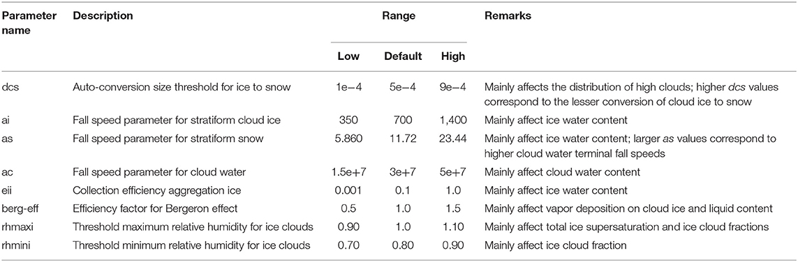
Table 1. Cloud microphysics and macrophysics parameters used in this study.

UQ Framework for Sensitivity Analysis and Bayesian Inference

Sensitivity Analysis

According to Sobol (1993), if a set of m-independent random parameters ξ = (ξ₁, …, ξ_m) produces response f(ξ), it can be written in the form of an expansion as follows:

$\begin{array}{l}f\left(\xi \right)=f_0+{\displaystyle \sum _{i=1}^m}{f}_i\left({\xi }_i\right)+{\displaystyle \sum _{i=1}^m}{\displaystyle \sum _{j>1}^m}{f}_{ij}\left({\xi }_i{\xi }_j\right)+\dots \\ +f_{1\dots ,m}\left({\xi }_1,\dots ,{\xi }_m\right)& (1)\end{array}$

where f₀ is the expected value of f(ξ), and f_{i1, …, is}({i₁, …, i_s}; s = 1, …, m) are orthogonal functions. This representation is commonly referred to as the variance decomposition analysis. The expected square of this decomposition (Equation 1) leads to the following variance decomposition of f(ξ):

$\begin{array}{ll}V={\displaystyle \sum _{i=1}^m}{V}_i+{\displaystyle \sum _{i=1}^m}{\displaystyle \sum _{j>1}^m}{V}_{ij}+\dots +V_{1\dots m}& (2)\end{array}$

where V is the total variance of f(ξ), V_i is the partial variance due to the perturbation of input parameter ξ_i alone, and V_{i1, …, is} is the partial variance due to the interactions between perturbed input parameters {ξ_i1, …, ..ξ_is}. Sobol's variance-based sensitivity indices are:

$\begin{array}{ll}{S}_{i_1,..,i_s}=\frac{V_{i_1,..,i_s}}{V}& (3)\end{array}$

The first-order sensitivity index (also called the main effect of ξ_i) is:

$\begin{array}{ll}{S}_i=\frac{V_i}{V}& (4)\end{array}$

Polynomial Chaos (PC) has been suggested as an efficient method for describing the stochastic processes required to quantify uncertainties in a given system (Ghanem and Spanos, 1991; Le Maitre and Knio, 2010). PC is based on a probabilistic paradigm that reflects the stochastic quantities of interest as a truncated PC expansion, also termed PCE. The PCE of a particular quantity of interest (QoI; see Table 2) is written as a function of m uncertain parameters [ξ = (ξ₁, ξ₂, …, ξ_m)] in the [−1, +1] space as follows:

$\begin{array}{ll}E\left(\xi \right)\approx {\displaystyle \sum _{k=0}^R}{e}_k{\psi }_k\left(\xi \right)& (5)\end{array}$

where E(ξ) is the desired QoI, e_k are the PCE coefficients, and ψ_k(ξ) are the multi-dimensional Legendre polynomials that form the following orthogonal basis:

$\begin{array}{l}<{\psi }_i,{\psi }_j>={\displaystyle \int }{\psi }_i\left(\xi \right){\psi }_j\left(\xi \right)\rho \left(\xi \right)d\xi ={\delta }_{ij}<{\psi }_i^2>,\end{array}$

where ρ(ξ) is the underlying uniform distribution.

TABLE 2

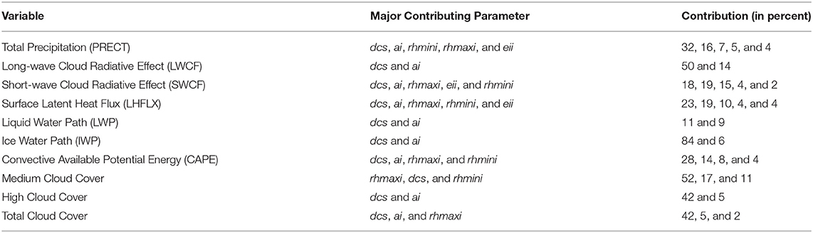
Table 2. First-order sensitivity contribution of parameters for different variables.

The expanded form of the PCE in Equation (5) can be written as follows:

$\begin{array}{l}E\left(\xi \right)=e_0{\psi }_0+{\displaystyle \sum _{i=1}^m}{e}_1{\psi }_1\left({\xi }_i\right)+{\displaystyle \sum _{i=1}^m}{\displaystyle \sum _{j\ge i}^m}{e}_{ij}{\psi }_2\left({\xi }_i,{\xi }_j\right)\\ +{\displaystyle \sum _{i=1}^m}{\displaystyle \sum _{j\ge i}^m}{\displaystyle \sum _{k\ge j}^m}{e}_{ijk}{\psi }_3\left({\xi }_i,{\xi }_j,{\xi }_k\right)+,\dots & (6)\end{array}$

The total number of expansion terms (R) in Equations 5 and 6 for m parameters and a PC order r is given by:

$\begin{array}{ll}R=\frac{\left(m+r\right)!}{m!r!}& (7)\end{array}$

The PC expansion in Equation (6) is similar to the decomposition in Equation (1) and thus provides a surrogate for approximating model outputs for a given set of parameters. Transforming Equation (6) into Equation (2) enables the corresponding sensitivity indices to be estimated (Crestaux et al., 2009).

PCE coefficients can be computed using two approaches: intrusive and non-intrusive. In the intrusive methods, the model equations are reformulated through the substitution of stochastic or random variables such that the model deploys the stochastic Navier Stokes Equation (e.g., Kusch and Frank, 2018). It is often challenging to compute the PC coefficients from an intrusive method since it involves source code modification (Ghanem and Spanos, 1991). Non-intrusive methods, on the other hand, use samples of model simulations for different realizations of parameters to build a surrogate model (Peng et al., 2014; Sraj et al., 2016). Herein, we used a non-intrusive spectral projection (NISP) method (Reagan et al., 2003; Constantine et al., 2012) to compute the PCE coefficient as follows:

$\begin{array}{ll}{e}_k=\frac{<E,{\psi }_k>}{{<\psi }_k{\psi }_k>}=\frac{1}{{<\psi }_k{\psi }_k>}{\displaystyle \int }E{\psi }_k\left(\xi \right)\rho \left(\xi \right)d\xi & (8)\end{array}$

The stochastic integral (Equation 8) is computed numerically using appropriate quadrature methods, as follows:

$\begin{array}{ll}<E,{\psi }_k>\approx {\displaystyle \sum _{q=1}^Q}E\left({\xi }_q\right){\psi }_k\left({\xi }_q\right)w_q& (9)\end{array}$

where Q is the total number of quadrature points, ξ_q denotes the vectors of the parameters at a quadrature point q, and w_q is the corresponding weight. The Smolyak sparse nested grid-based quadrature method (Smolyak, 1963) was used to reduce the number of SCAM6 runs to build the surrogate model. In this study, for a PC order with r = 4 and m = 8 parameters (i.e., total truncated PCE terms R = 495), the total number of quadrature points created from the Smolyak level 5 was 3937 (see http://www.sparse-grids.de/ and Smolyak, 1963 for full details of the Smolyak quadrature).

Figure 1 shows the spectrum of normalized PCE coefficients $\left(\frac{e_k}{e_0}\right)$ calculated from a non-intrusive spectral projection (NISP; see Equation 8), and the vertical solid lines separating PCE terms according to their PC order (r = 4; 1, 2, 3, 4). This indicates that PC does not converge properly since the estimated PCE coefficients increase instead of decaying with an increase in PC order, suggesting an overfitting of the model output. This is due to internal noise in model simulations that is not tolerated by the NISP method when calculating PCE coefficients (Peng et al., 2014; Sraj et al., 2016). We thus opted to use a non-intrusive technique based on compressed sensing (CS; Chen and Donoho, 1994; Van den Berg and Friedlander, 2007, 2009) to estate more suitable PCE coefficients.

FIGURE 1

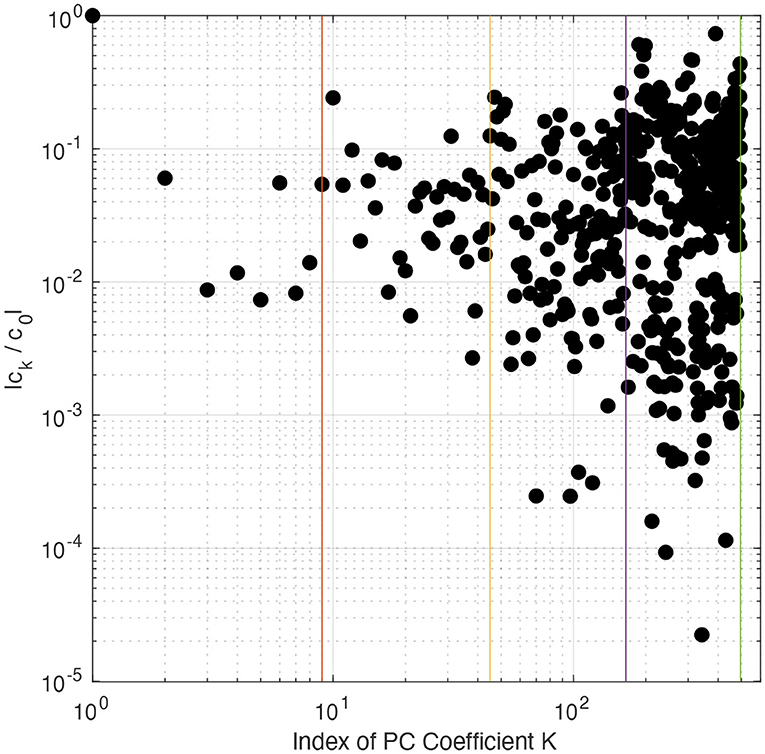
Figure 1. PCE normalized coefficients c_k/c₀ for PC of order up to r = 4. Vertical lines separate the PCE terms into their different PC orders. PCE coefficients were calculated using the non-intrusive spectral projection (NISP) method.

CS estimates the noise in the data to be fitted and then approximates them using a PC representation that tolerates the corresponding noise level. In this case, CS solves Equation (5) by exploiting the approximate sparsity of its signal, which is set by the l1 norm. CS with the l1 norm is known as BPDN.

Thus, if we consider E = [E(ξ₁), E(ξ₂), ….., E(ξ_Q)] as the vector of model evaluations at different quadrature nodes (ξ_q), e = (e₀, e₁, ….., e_R) as the vector of PCE coefficients, and ψ as the PC basis functions evaluated at each sampled ξ_q, then an equivalent of Equation (5) could be written as follow:

$\begin{array}{ll}E=\psi e& (10)\end{array}$

The CS seeks a solution of Equation (10) with the minimum number of non-zero entries by solving the optimization problem:

$\begin{array}{ll}\frac{minimize}{e}{\left|\right|e\left|\right|}_1:{\left|\right|E-\psi e\left|\right|}_2\le \delta & (11)\end{array}$

where δ is noise, estimated by cross-validation (see Peng et al., 2014). Equation (11) was solved using a standard l1-minimization solver based on a spectral projection gradient algorithm (Van den Berg and Friedlander, 2009) provided in the SPGL1 MATLAB package by Van den Berg and Friedlander (2007) (see https://friedlander.io/spgl1/ for full details). The optimization problem (Equation 11) was solved using the previously simulated 3937 SCAM6 simulations. The resulting normalized PCE coefficients (e_k/e₀) are shown in Figure 2; their spectrum shows a decaying trend. In BPDN, the decrease in the PCE coefficients eventually reaches a plateau, while a further increase in the PC order leads to minimal improvement in the accuracy of the surrogate model. In light of these results, we used the BPDN approach to build the surrogate model (Equation 10).

FIGURE 2

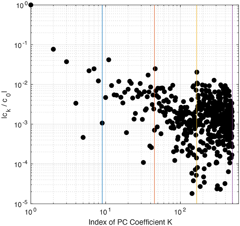
Figure 2. PCE normalized coefficients c_k/c₀ for PC of order up to r = 4. Vertical lines separate the PCE terms into their different PC orders. PCE coefficients were calculated using the basis pursuit denoising (BPDN) method.

Figure 3 shows the scatter plot of SCAM6 simulations against results from the surrogate model built using PCE and BPDN for various variables or quantity of interest (QoI). The surrogate model and SCAM6 both show linear relationships for various QoIs and the constructed PCE model reproduces well the mean of the deterministic model signal. To quantify the level of agreement between SCAM6 and the surrogate model, we computed the R²-value to estimate the fraction of total variance in SCAM6 results explained by the surrogate model. The highest R²-value (0.99) were obtained for the longwave cloud radiative effect (LWCF) and the lowest value (0.79) for the convective available potential energy (CAPE) (Figure 3). The R²-values of the remaining variables, including cloud water path (CWP), liquid water path (LWP), total cloud fraction (CLDTOT), surface latent heat flux (LHFLX), shortwave cloud radiative effect (SWCF), and total precipitation (PRECT) ranged between 0.79 and 0.99, indicating that BPDN enables to successfully build a surrogate model that is capable of describing the desired QoIs.

FIGURE 3

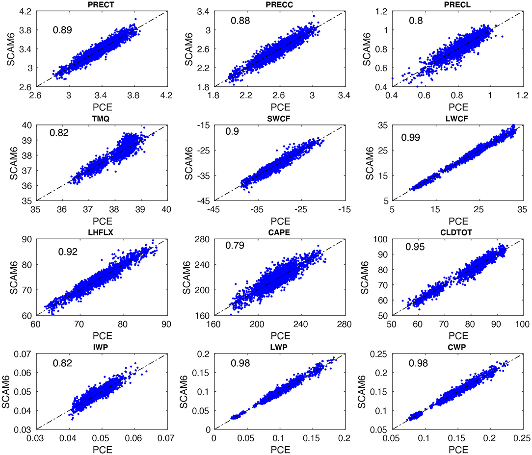
Figure 3. Scatter plots of PC-fitted outputs vs. SCAM6 simulations for various climate variables. Row 1 corresponds to total precipitation (PRECT), convective precipitation (PRECC), and large-scale precipitation (PRECL). Row 2 corresponds to total precipitable water (TMQ), shortwave cloud radiative effect (SWCF), and longwave cloud radiative effect (LWCF). Row 3 corresponds to latent heat flux (LHFLX), convective available potential energy (CAPE), and total cloud cover (CLDTOT). Row 4 is similar to the previous rows but for ice water path (IWP), liquid water path (LWP), and cloud water path (CWP). The fraction (0–1) of the total variance of SCAM6 simulations explained by the PC-based surrogate model for various climatic variables is indicated by numbers in the upper left of each panel.

Bayesian Inference

The posterior probability density function (PDF) of the CMP parameters can be calculated by updating the prior PDF according to Bayes' rule. Let $d={(d_1,d_2,...d_n)}^T$ be a vector of observation, $p={(p_1,p_2,...p_n)}^T$ a vector of uncertain input parameters, and G a forward model such that d ≈ G(p). The prior PDF [π(p)], which represents a priori information about p, is assumed to be uniform (non-informative, i.e., $\pi (p)={\prod }_{i=1}^{n_p}\frac{1}{(b_i-a_i)}$, such that a_i and b_i are, respectively, the lower and upper bounds of parameter p_i; Table 1]. The input parameters p are assumed to be independent with respect to one another. According to Bayes' rule, the posterior [π(p|d)] is proportional to the product of the likelihood [L(d|p)] and the prior as:

$\begin{array}{ll}\pi \left(d\right)\propto L\left(p\right)\pi \left(p\right)& (12)\end{array}$

The likelihood is obtained from a cost function E(p) using a Taylor score (TS, Taylor, 2001) and a scaling factor S (used to normalize the cost function). Gaussian likelihoods based on misfits [i.e., the exponential form of the mean-square errors (MSE)] are widely adopted as cost functions (e.g., Sraj et al., 2016; Qian et al., 2018). Thus, to consider both the misfit in magnitude and the mismatch in the vertical cloud distribution, we used [ln(TS)]² as the cost function (Guo et al., 2015; Qian et al., 2018) with a theoretical range of (0, infinity).

$\begin{array}{ll}\pi \left(d\right)\propto expexp\left[-E\left(p\right)\right]{}^{*}\pi \left(p\right)& (13)\end{array}$

$\begin{array}{ll}E\left(p\right)=S.{\left\{\text{ln ln }\left[TS\left(p\right)\right]\right\}}^2& (14)\end{array}$

The TS used to evaluate model performance in terms of standard deviation and correlation with respect to observations is given as follows:

$\begin{array}{ll}TS=\frac{{(\frac{{\sigma }_{model}}{{\sigma }_{obs}}+\frac{{\sigma }_{obs}}{{\sigma }_{model}})}^2{\left(1+VC{C}_0\right)}^k}{4{\left(1+VCC\right)}^k}& (15)\end{array}$

$\begin{array}{ll}VCC=\frac{{\displaystyle {\sum }_{i=1}^v}{w}_i\left(d_{i,model}-G{M}_{model}\right)\left(d_{i,obs}-G{M}_{obs}\right)}{{\sigma }_{model}.{\sigma }_{obs}.{\displaystyle {\sum }_i^v}{w}_i}& (\mathrm{15a})\end{array}$

$\begin{array}{ll}\sigma =\sqrt{\frac{{\displaystyle {\sum }_{i=1}^v}{w}_i{\left(d_i-GM\right)}^2}{{\displaystyle {\sum }_{i=1}^v}{w}_i}}& (\mathrm{15b})\end{array}$

$\begin{array}{ll}GM=\frac{{\displaystyle {\sum }_{i=1}^v}{w}_i{d}_i}{{\displaystyle {\sum }_{i=1}^v}{w}_i}& (\mathrm{15c})\end{array}$

where subscripts “obs” and “model” denote the observed and simulated results, respectively. The standard deviation and vertical correlation coefficients between the observed and simulated results are denoted by σ and VCC, respectively. VCC₀ denotes the maximum possible vertical correlation between the observations and the model outputs, and k indicates a value that controls the correlation of the relative weight of the vertical level compared to the standard deviation in TS (Equation 15). VCC₀ and k were set to 1 and 4, respectively, following Yang et al. (2013). A lower TS value is an indicator of better model performance, and model prediction and observation are considered identical when TS = 1. Vector d represents the observed vertical cloud distribution from ARM97, w_i is the vertical weight of a level, and n is the number of vertical levels. The scaling factor was chosen as

$\begin{array}{ll}S=\frac{2}{\Delta }& (16)\end{array}$

Jackson et al. (2004) noted that the spread of the cost function (i.e.,) due to natural variability could be used for its normalization (see Equation 14). In general, the natural variability is estimated via multiple model runs (Decremer et al., 2015). In this study, the average of all original simulations corresponding to the set of perturbed parameters was considered as an indicator of the spread of model bias due to natural variability (Qian et al., 2018). The Bayesian formulation thus requires the evaluation of the posterior distribution (Equation 13) to estimate the uncertain parameters. To this end, we employed a Markov Chain Monte Carlo (MCMC) technique; however, such an approach requires a large number of posterior evaluations in order to reach a meaningful solution. Each posterior evaluation requires a single model simulation, which is computationally prohibitive. Therefore, the PC-based surrogate model was used within the random-walk Metropolis MCMC algorithm to generate the 50,000 samples from posterior distributions for each parameter (Metropolis et al., 1953).

Results and Discussion

Relative Importance of Sensitive Parameters

Figure 4 shows the contribution of first-order sensitivity for each parameter, the total second-order interactive effect (int²) between any two-input parameters, and higher-order interactive effects (int^h) between more than two-input parameters, to the total explained variance for specific QoIs as resulting from the PCE surrogate model. The total variance explained by first-order and interactive effects ranges between 80 and 99% (Figure 4), as reflected by the R² values for different QoIs (Figure 3). In Figure 4, int² indicates the impact of a parameter on the model simulation depending on a second parameter, while int^h corresponds to the impact of a parameter on the model simulations depending on more than two parameters. The contribution of first-order effects (in percent) to the total explained variance from different parameters are presented in Table 2. We found that dcs contribution is highest, about 32, 50, 18, 23, 11, 84, and 28% for PRECT, LWCF, SWCF, LHFLX, LWP, IWP, and CAPE, respectively. dcs also contributes about 17, 42, and 42% for the medium-level cloud (CLDMED), the high-level cloud (CLDHGH), and for the total cloud (CLDTOT), respectively. The total int² and int^h effect contributed significantly to the total variance. For example, in PRECT, LWCF, SWCF, LHFLX, LWP, IWP, CAPE, CLDMED, CLDHGH, and CLDTOT, the int² was about 8, 3, 8, 7, 15, 4, 8, 7, 3, and 3%, respectively, while the corresponding int^h values were about 15, 27, 20, 20, 30, 4, 10, 6, 43, and 43% (Figure 4).

FIGURE 4

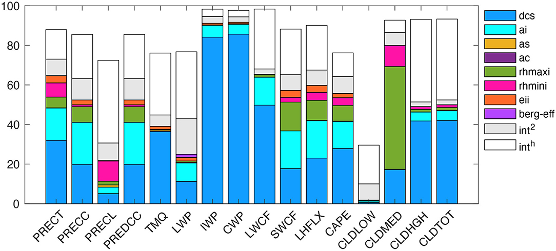
Figure 4. Relative contributions of variance for individual parameters (main effect) to the overall variance of different climatic variables. The total contribution of variance from the second-order (two-way) interaction between parameters is indicated by the gray box in the bar plot (Int²); the remainder of the contribution to variance from the higher-order (i.e., order > 2) interactions among other parameters is indicated by a white box for each variable.

In addition to the total int² effect, we also attempted to determine how effects induced by a single parameter may be amplified or suppressed by other parameters, compared to their OAT sensitivity (Zhao et al., 2013). As shown in Figure 5, we found that the interactive effects between any two-input parameters are not consequent (<3%) for most of the simulated variables, with the exception of the interactive effect between dcs and ai, which shows a prominent contribution of ~4% to PRECT, 10% to LWP, and ~4% to SWCF. Although the contributions of any two-parameter interactions are low relative to individual contributions, the large number of int² (28) makes their total int² contribution from all parameter pairs noteworthy (Figure 4).

FIGURE 5

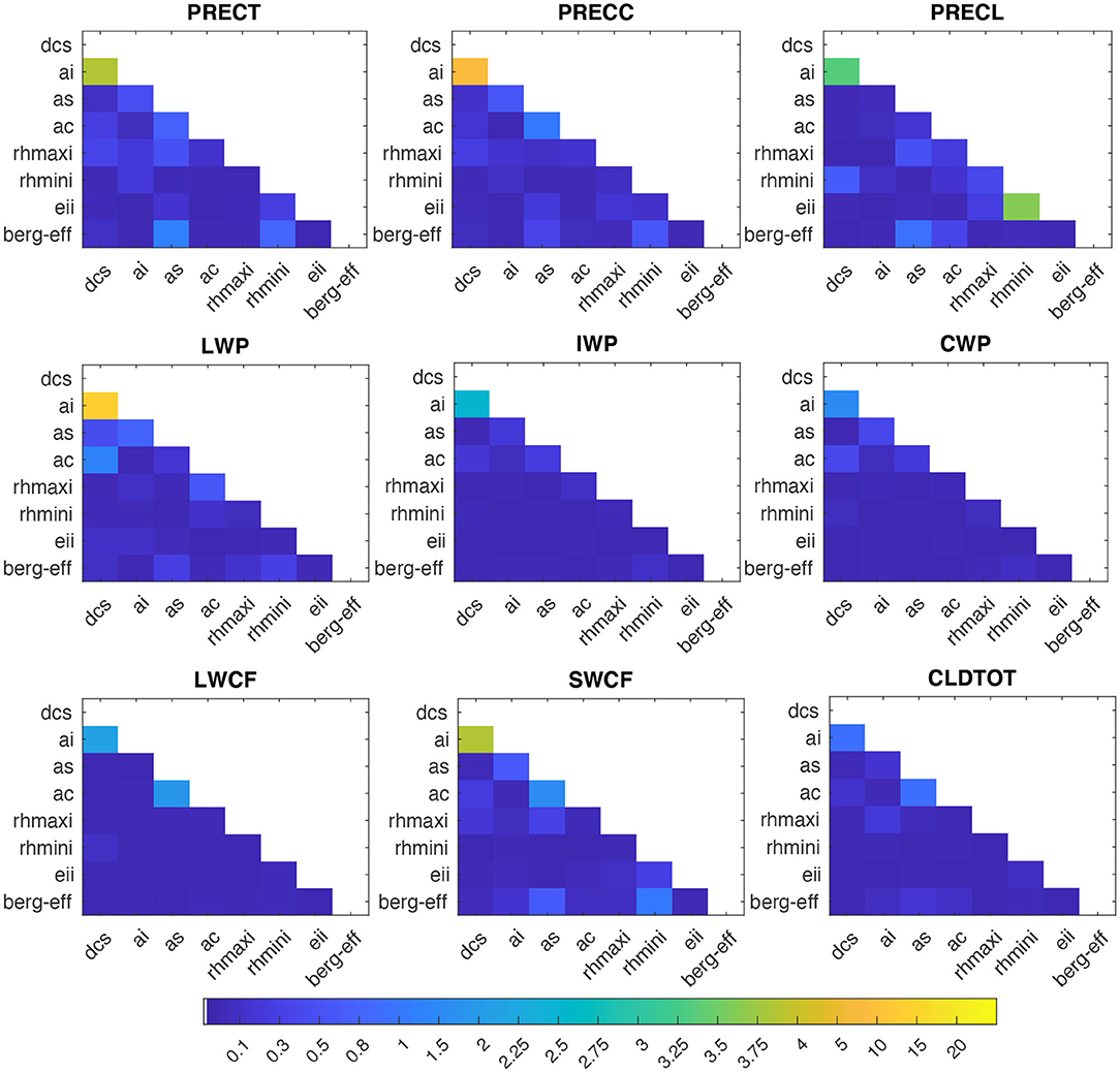
Figure 5. Relative contributions (in %) from the interaction of a parameter with other parameters, to the total variance of PRECT, PRECC, and PRECL (in the first row), LWP, IWP, and CWP (in the second row), and LWCF, SWCF, and CLDTOT (in the third row), as estimated using the PC-fitted method.

In order to identify the overall most sensitive parameters, we quantified the total effects, including their first-order, int², and int^h contributions (Figure 6). The total sensitivity for dcs ranges from 40 to 80%, ai from 15 to 30%, and the three-parameter combination (rhmaxi, rhmini, and eii) from 5 to 15% with respect to different simulated QoIs. The total sensitivity of some of these parameters is insensitive, for example, as, ac, and berg_eff, which contribute <3% to most simulated QoIs, with the exception of as, which contributed 2–5% to certain variables. Thus, dcs, ai, rhmaxi, eii, rhmini, and as were identified as the most influential parameters in CMP parameterization, arranged in decreasing order of their total sensitivity.

FIGURE 6

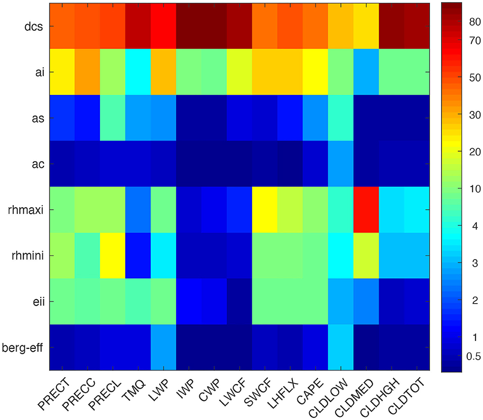
Figure 6. Total contribution of each parameter to the total explained variance (in %) from PC-fitted outputs against SCAM6 simulations for various climatic variables. A larger number indicates greater significance.

Response of Simulated QoI to Sensitive Parameters

According to the parameter sensitivities results presented in section Relative Importance of Sensitive Parameters, we explain the response characteristics of different QoIs to different parameters based on the 3,937 SCAM6 simulations. The characteristics of the response of different QoIs to a parameter are examined by analyzing the perturbation effect of a parameter while keeping the remaining parameter values fixed at their mean value (i.e., zero in a ±1 uncertainty range). We found that the substantial increase in CLDHGH (~64 to 83%) and the partial increase in CLDMED (~19 to 28%) following an increase in dcs (Figure 7) may have occurred because increasing dcs typically reduces the ice to snow conversion and thus increases the ice particle content of the upper atmosphere. Further, this increase in ice particles in the upper atmosphere following an increase in dcs leads to an increase in IWP (~0.02 to 0.12 kg/m²), LWCF (~10 to 25 W/m²), and SWCF (−26 to −33 W/m²), and to a decrease in LWP (~0.054 to 0.045 kg/m²) (Figure 8). A decrease in PRECT (~3.7 to 3.1 mm/day) in response to an increase in dcs is also noted (Figure 9), which indirectly alters (decreases) the stability of the atmosphere (CAPE; Figure 7) and thus the convective precipitation (PRECC; Figure 9), since changes occur in CMP but not in convection parameterizations. This phenomenon was also reported for different CMP parameters by Lin et al. (2016) and Pathak et al. (2020). In addition, the increase in ai caused more ice particles to fall, thereby decreasing CLDHGH (~85 to 78%), LWCF (~30 to 19 W/m²) and SWCF (−35 to −29 W/m²), and IWP (0.1 to 0.06 kg/m²) (Mitchell et al., 2008), while causing an increase in LWP from 0.044 to 0.049 kg/m² (Figures 7, 8). The ai also affects atmospheric instability, which typically increases with increasing ai (Figure 7), causing an increase in PRECT from ~3.1 to 3.4 mm/day (Figure 9; Sun et al., 2011; Yang et al., 2013; Pistotnik et al., 2016). The effects of ai on LWCF are small when compared to the effect of dcs; this could reflect the small changes in CLDHGH that cause an increase in ai. In general, an increase in dcs increases the concentrations of ice clouds, whereas an increase in ai decrease ice cloud concentrations, hence the increased and decreased albedo effects leading, respectively, to increasing and decreasing SWCF.

FIGURE 7

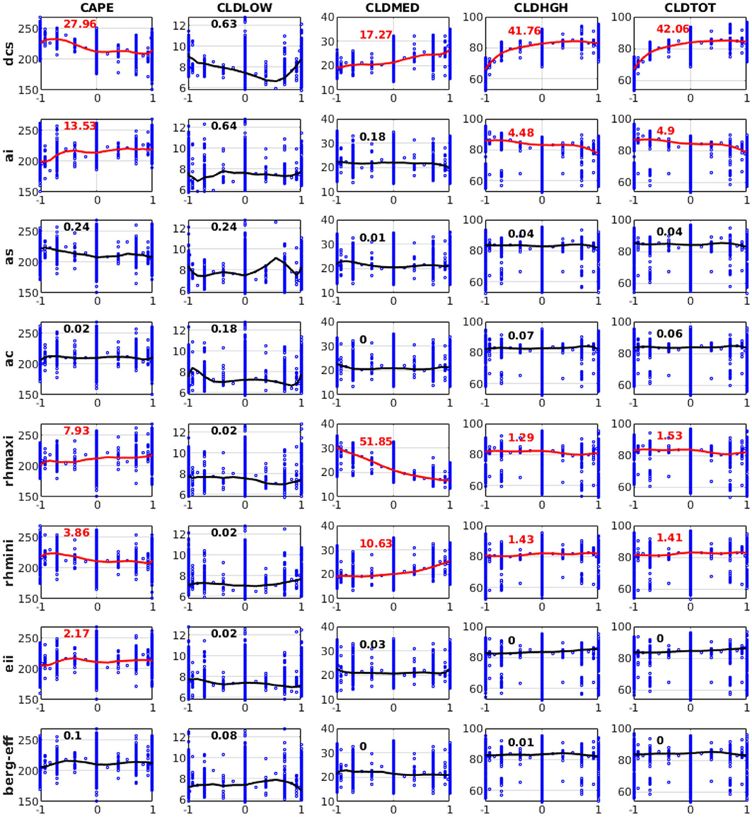
Figure 7. Variation of convective available potential energy (CAPE), low-level cloud (CLDLOW), medium-level cloud (CLDMED), high-level cloud (CLDHGH), and total cloud cover (CLDTOT) in response to perturbations of eight different parameters from 3,937 SCAM6 simulations. The numbers in each plot represent the relative contributions (in %) of each input parameter perturbation to the overall variation of different variables. Red indicates that the contribution is significant (F-test) at the 95% significance level. The line in each plot corresponds to the response effect of the perturbation of a single parameter, keeping all other parameters at the zero (central) position of the parameter uncertainty range for the simulation of that variable. Vertical bars show the range in the variation of values of a particular variable in response to the perturbation of other parameters.

FIGURE 8

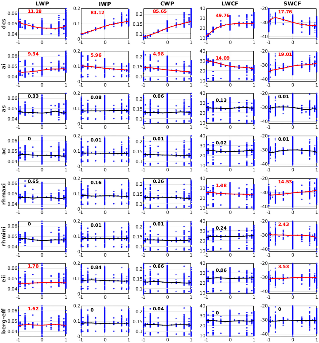
Figure 8. Variation of liquid water path (LWP), ice water path (IWP), cloud water path (CWP), longwave cloud radiative effect (LWCF), and shortwave cloud radiative effect (SWCF) in response to perturbations of eight different parameters from 3,937 SCAM6 simulations. The numbers in each plot represent the relative contributions (in %) of each input parameter perturbation to the overall variation of different variables. Red indicates that the contribution is significant (F-test) at the 95% significance level. The line in each plot corresponds to the response effect of the perturbation of a single parameter when all other parameters at maintained at the zero (central) position of their uncertainty range for the simulation of that variable. Vertical bars denote the range of variation in values of a particular variable in response to the perturbation of other parameters.

FIGURE 9

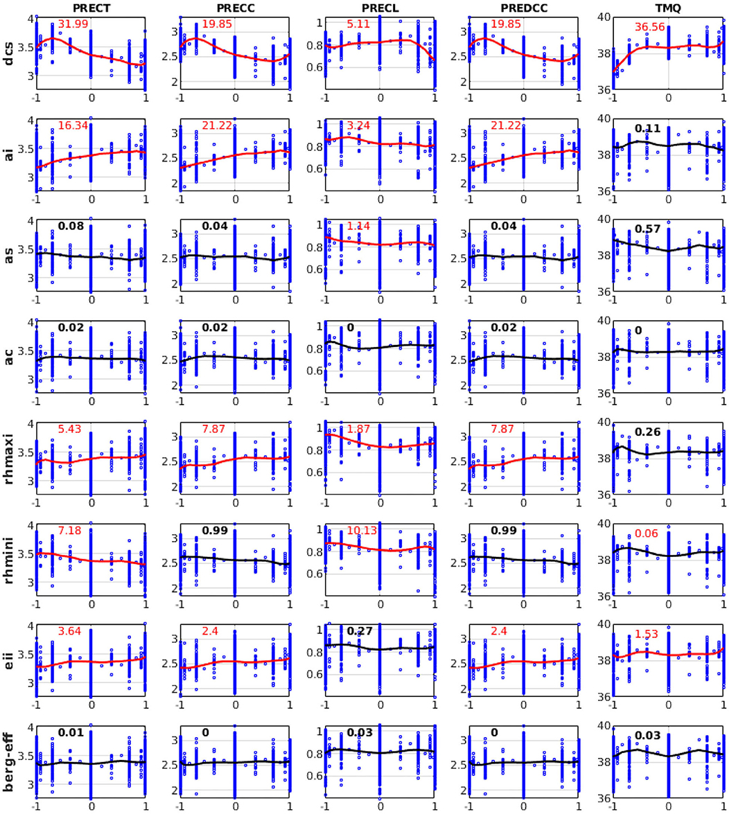
Figure 9. Variation of PRECT, PRECC, PRECL, deep convective precipitation (PREDCC), and total precipitable water (TMQ) in response to perturbations of eight different parameters from 3,937 SCAM6 simulations. The numbers in each plot represent the relative contributions (in %) of each input parameter perturbation to the overall variation of different variables. Red denotes that the contribution is significant (F-test) at the 95% significance level. The line in each plot corresponds to the response effect of the perturbation of a single parameter when keeping all other parameters at the zero (central) position of their uncertainty ranges for the simulation of that variable. Vertical bars show the range of variation for values of a particular variable in response to the perturbation of other parameters.

Further, the increase in rhmaxi decreases both the grid box of full ice cloud cover (i.e., 100%) and clouds that reach supersaturation, leading to a large decrease in CLDMED (30 to 16%). A substantial decrease in CLDHGH was also found; however, due to lower temperatures in the upper atmosphere compared to the mid-level atmosphere, supersaturation was somewhat counterbalanced. The moderate increase in PRECT from 3.3 to 3.45 mm/day and decrease in SWCF from −31 to −29 W/m² were thus the main reasons behind the observed increase in rhmaxi (Figures 7–9; Xie et al., 2018). Additionally, the increase in rhmini reduced the fractional ice cloud cover formation and thus somewhat increased the presence of liquid clouds, as shown by the increase in CLDMED from 19 to 26% (Figure 7). We do not show here the response for CLDLOW since this was relatively insensitive to CMP parameters; its variation could be due to the control of frontal clouds and precipitation over the SGP site in addition to local convection (Qian et al., 2015).

Furthermore, we evaluated the response characteristics of the vertical distribution of different variables in Figure 10 and the response characteristics of their vertical averages (from the surface to 100 hPa) in Figure 11. In Figure 10, the color bar values for each panel plot are not shown; however, the highest to lowest values are indicated by the dark yellow to the dark blue colors of the contour plot. This suggests that the average value of (a) snow concentration (maximum at ~400 hPa with a spread between 600 and 200 hPa; Figure 10) decreases with increasing dcs for the first half of the parameter space, and (b) cloud liquid concentration (primarily concentrated between the surface and 600 hPa; Figure 11) significantly changes non-linearly relative to dcs; generally, it decreases for the first 45% of the parameter space and increases for the last 45% of the parameter space) and to as (sensitive only to the last 50% of the parameter space, initially increasing but later decreasing) (Figure 11). Furthermore, we note that the vertical average of cloud ice concentration (maximum at about 225 hPa with a spread from 300 to 150 hPa) increases significantly due to increasing dcs but decreases with increasing ai. The rate at which cloud condensate is converted to precipitation (maximum at ~450 hPa with a spread from 300 to 700 hPa; Figure 10) decreases significantly with increasing dcs (Figure 11). The vertical averages of longwave cloud radiative effect (maximum at about 350 hPa and 100 hPa) and shortwave cloud radiative effect (centered at about 250 hPa) are primarily sensitive to dcs and ai in the first 60% of the parameter space. In general, shortwave and longwave cloud radiative effect increase with increasing dcs and decrease with increasing ai (Figure 11). Additionally, the vertical average of relative humidity (maximum at about 300 hPa with a spread from 500 to 200 hPa) increases monotonically due to increasing dcs, rhmaxi, and rhmini, and decreases due to increasing ai. The vertical average of specific humidity, which is primarily distributed from the surface to 800 hPa, increases with increasing dcs and decreases with increasing as within the first 45% of parameter space; it also decreases monotonically with increasing ai in the last 60% of the parameter space (Figure 11). Thus, the increase in radiative effect with increasing dcs supports our finding of an increase in LWCF and SWCF, as well as the increase in ice cloud concentration with increasing dcs, which supports the substantial increase in IWP. Finally, the decrease in the rate of conversion of cloud condensate to precipitation with increasing dcs supports the corresponding reduction in PRECT through a reduction in its instability (Figures 7, 9).

FIGURE 10

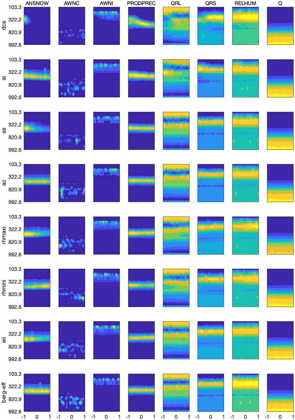
Figure 10. Parameter perturbation response to the vertical distribution of snow concentration (ANSNOW), cloud water concentration (AWNC), ice concentration (AWNI), precipitation production (PRODPREC), longwave heating rate (QRL), shortwave heating rate (QRS), relative humidity (RELHUM), and specific humidity (Q).

FIGURE 11

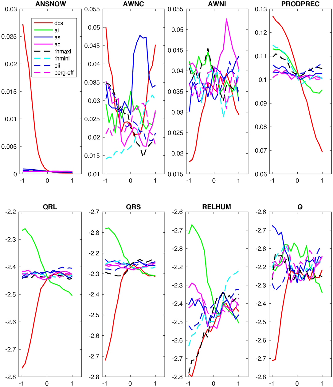
Figure 11. Parameter perturbation responses to vertically averaged (surface to 100 hPa) variables (ANSNOW, AWNC, AWNI, PRODPREC, QRL, QRS, RELHUM, and Q).

Bayesian Inference

Finally, we analyze the Bayesian inference results for estimating CMP parameters. The MCMC algorithm (Metropolis et al., 1953) was used to generate sample chains for the different CMP parameters. We have run five times, each for 10,000 iterations (or samples), with different initial parameter values for efficient samples mixing and convergence. The PCE surrogate model was used to evaluate the cost function for each MCMC chain to reduce the computing requirements. Figure 12 shows the trace plot of the CMP parameters (chains vs. MCMC iteration number), indicating a well-mixed chain. This implies that the distribution of the chains will remain unchanged with further sampling and converged to a stationary distribution. The average acceptance rate of MCMC samples was found to be 35%. From Figure 12, we find that the parameter samples of dcs, ai, as, ac, rhmaxi, rhmini, berg_eff move around their default CMP values. The parameter samples for eii, on the other hand, did not move around the default value, but rather skewed leftward to the default value to cover a larger part of the prior range, resulting in a wider posterior.

FIGURE 12

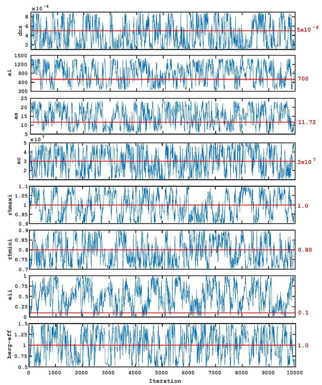
Figure 12. Chains of parameters from MCMC samples. The horizontal red line (and the value shown in red) indicate the default parameter value used in NCAR SCAM6.

Further, we computed the marginalized posterior distribution from the MCMC chains by discarding the first 500 iterations (to begin with a good starting point of MCMC run) using kernel density estimates (KDE; Silverman, 1986). The marginalized posterior PDF for each parameter along the diagonal of the eight-by-eight matrix shows that the posterior PDFs of dcs, ai, as, rhminl, and berg_eff exhibit a sharp increase but are skewed leftward for dcs and rightward for ai and as relative to the default CMP value (Figure 13). Thus, with respect of the default values for dcs, ai, and as (0.0005, 700, and 11.72), their posterior mean estimates are found to be 0.0004, 903, 14.85, respectively, while those of rhminl and berg_eff are found to be 0.79 and 1.03, respectively, close to their default values of 0.80 and 1.0. The posterior mean estimates of these parameters are also found falling within the acceptable ranges (i.e., within the 95% of the intervals of high posterior probability). The posterior PDFs of ac, rhmaxi, and eii do not show a sharp peak and are mostly flat, consistent with our conclusions from their chains (Figure 12) and indicating less-informative posteriors, which is likely due to the lack of relevant observations.

FIGURE 13

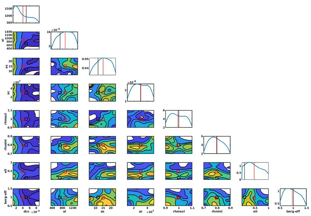
Figure 13. Probability Distribution Functions (PDFs) of parameters using KDE along the diagonal of the matrix. The contour plots show the joint PDFs of two parameters. The black and red vertical lines show the default and posterior mean parameter values.

The examination of 1D posterior PDFs provides only a measure of the integrated influence of parameters on model output; specific functional dependence is hidden. Thus, in addition to 1D posterior PDFs, we also show 2D PDFs, which facilitate parameter space visualization and the identification of optimized parameter sets. We found that the cost function for a parameter choice is strongly dependent on the other parameter chosen (Posselt, 2016). For example, the 2D PDF for rhmaxi and as, which exhibits a linear response, suggests an increase in cost function with an increase in both rhmaxi and as. We also found some parameters whose two-dimensional PDFs do not show any significant variations with changes in the other parameters, indicating that the cost function is functionally independent (e.g., the 2D PDF of eii does not show any significant changes when other parameters are changed).

To examine the extent to which the parameters posterior distributions inferred by the proposed UQ framework provide useful information, we assessed whether the posterior mean parameters can improve a global climate model performance. We therefore performed two sets of 7 year global climate simulations; one using the default parameters, and the other using the the posterior mean parameters. Both simulations are conducted using the CESM2 model with prescribed observed climatological sea surface and sea-ice temperatures. The simulation with posterior mean parameters suggests an overall improvement of ~7% over the globe in annual means, with the largest improvement of ~15% over the global land for December-February (Figure 14). The simulation of individual climate variables (e.g., total precipitation, cloud distribution, cloud radiative effect, and humidity) are improved by 5 to 50% over the globe, as well as over the tropical and sub-tropical regions, across the different periods (i.e., annual, June-August, and December-February), in comparison to the default model simulation (Figure 14). However, over the polar region, some of the simulated variables with the posterior mean parameters values have deteriorated by 5 to 20% compared to the default model simulation. In our setting, posterior parameters distributions were inferred from data collected in subtropics at the Southern Great Plains (36°N and 97°W; Zhang et al., 2016), and as such the resulting parameters are calibrated for such regions, which also explains the improvement we obtained in the subtropics and tropics. Recent results (Pathak et al., 2020) suggest a spatial dependency of some of the considered parameters despite being prescribed as constant values across the globe. Our results over the polar regions also support the use of spatially varying cloud parameters in climate models, which will be explored in depth in our future work.

FIGURE 14

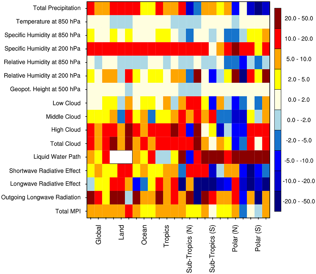
Figure 14. The Model Performance Index (MPI in percent) resulting from simulations of various climate variables over the global, tropics (30°N−30°S), norther subtropics (30–60°N), southern sub-tropics (30–60°S), northern polar (60–90°N), and southern polar (60–90°S) regions, across different periods [i.e., Annual (ANN), June-August (JJA), December-February (DJF)]. The MPI is constructed using a metric developed by Zhang (2015). The contours in color show the percentage improvement (positive values) or deterioration (negative values) for different climate variables from the simulation with posterior mean parameters with respect to the default model simulation. Total MPI—model performance as averaged over all climate variables. Following observations and reanalysis data are used for construction of this metrics, the Global Precipitation Climatology Project (Adler et al., 2003) for total precipitation, the Clouds and Earth's Radiant Energy System-Energy Balanced and Filled (Loeb et al., 2009) project for shortwave and longwave radiative effect, the National Aeronautics and Space Administration Water Vapor Project (Randel et al., 1996) for liquid water path over ocean, and the International Satellite Cloud Climatology Project (Young et al., 2018) for low, middle, high, and total cloud, the ECMWF Interim reanalysis (Dee et al., 2011) for humidity, temperature, and geopotential height.

Conclusions

This study used an efficient multi-objective UQ framework to assess the sensitivity of NCAR SCAM6 outputs to cloud microphysics and macrophysics (CMP) parameterization schemes. The framework involved building a surrogate model using a polynomial chaos expansion, sensitivity analysis, and Bayesian inference to identify and quantify the uncertainties of various (quantities of interest) QoIs from the NCAR SCAM6 model associated with CMP parameterizations. The basis pursuit denoising (BPDN) approach was applied to build the polynomial chaos expansion (PCE) model to mitigate for internal noise in model simulations. The surrogate model was shown to realistically approximate the model outputs, explaining most of the variance of different QoIs, with the highest explained variance (about 99%) for longwave cloud radiative effect (LWCF) and the lowest explained variance (about 79%) for convective available potential energy (CAPE).

The UQ analysis suggested that the simulated QoIs are most sensitive to five (dcs, ai, rhmaxi, rhmini, and eii) of the eight CMP parameters. dcs alone contributed 40–80% of the total variance of different simulated QoIs, ai 15–30%, and rhmaxi, rhmini, and eii each contributed 5–15%. Parameters as, ac, and berg_eff were found to be the least sensitive, each of which contributed <5% to the total variance. Further splitting the total sensitivity effect of a parameter into first-, second-, and higher-order sensitivities, we found that the first-order sensitivity of dcs, ai, rhmini, rhmaxi, and eii together contribute more than 60% of the total variance in different QoIs. While, the second- and higher-order sensitivity of dcs, ai, rhmini, rhmaxi, and eii together contribute about 7 and 20% of the total variance in different QoIs. Some previous studies using the predecessor version of this model have also argued that dcs and ai are the most sensitive parameters for the simulation of total precipitation over the tropical region (He and Posselt, 2015; Qian et al., 2015; Zhang, 2015; Pathak et al., 2020). Other studies that employed different models have also suggested dcs and ai to be highly sensitive to cloud distribution (e.g., Bony and Dufresne, 2005; Sanderson et al., 2008; Golaz et al., 2011; Gettelman et al., 2012). The sensitivity of rhmaxi to cloud distribution was also reported in the E3SM model (Qian et al., 2018; Xie et al., 2018). Uncertainties in these parameters are considered as important factors in climate model sensitivity (Zelinka et al., 2020).

We also found that an increase in dcs increases the concentration of ice between 300 and 150 hPa (and vice versa for snow concentrations) by decreasing the conversion rate of ice to snow, which causes a substantial increase in cloud cover. This leads to significant increase in ice water path (IWP), LWCF, and SWCF. Furthermore, the increase in longwave and shortwave heating rates due to increased dcs were shown to sustain the corresponding increases in LWCF and SWCF. A significant decrease in total precipitation (PRECT) occurred due to an increase in dcs, which indirectly affected (decreased) the conversion of cloud condensate to precipitation; this was clear from the reduced instability, i.e., the CAPE and reduced convective precipitation. The decrease in the conversion of cloud condensate to precipitation due to an increase in dcs also reduced the liquid water path (LWP), as noticed from reduced cloud water concentrations. The possible physical mechanism behind the sensitivity of QoIs with respect to ai values seems to work oppositely to dcs. In addition, an increase in relative humidity occurred in response to increased dcs, rhmaxi, and rhmini. A decrease (increase) in cloud water concentration in response to an increase in rhmaxi (rhmini) was also reported. The impact of rhmaxi and rhmini on PRECT was identified through studying its effects on middle clouds (CLDMED). Generally, CLDMED decreases (increases) due to increasing rhmaxi (rhmini).

The Bayesian inference results for vertical cloud distribution showed that the Markov chain Monte Carlo (MCMC) chains for dcs, ai, as, ac, rhmaxi, rhmini, and berg_eff fluctuated around their default CMP values. However, for eii, the MCMC chains did not fluctuate around the default value but were skewed largely leftward; suggesting a non-informative cost function. The marginalized posterior distributions of the MCMC chains for dcs, ai, as, rhminl, and berg_eff showed well-defined peaks. The corresponding posterior mean estimate values were, respectively, found to be 0.0004, 903, 14.85, 0.79 and 1.03, compared to the corresponding default values of 0.0005, 700, 11.72, 0.80 and 1.0. The marginalized posterior distributions for ac, rhmaxi, and eii were mostly flat, indicating the probability of being nearly uniform across the parameter space; consequently, they do not provide meaningful information to estimate their posterior means. Global climate simulations performed using the posterior mean and default parameters have shown that the climate simulations using the posterior mean parameters values suggest an overall-improvement of ~7% over the globe in annual means. The largest improvement of ~15% was obtained over the global land for December-February. Specifically, the climate simulations using the posterior mean parameters values were improved over the tropical and sub-tropical regions, whereas it has deteriorated over the polar region. In line to the findings of Pathak et al. (2020), we anticipate that this deterioration in polar regions could be due to a spatial dependency of some of the considered parameters despite being prescribed as constant values across the globe in the climate models. Furthermore, the functional linear dependence of rhmaxi on as was also noted from the joint probability distribution of both parameters. This provides important information for understanding cloud processes and their associated physical processes and will assist developers in further improving climate models.

Data Availability Statement

The raw data supporting the conclusions of this article will be made available by the authors, without undue reservation.

Author Contributions

RP, HD, AS, SS, SM, OK, and IH identified the problem and designed the work to meet the objective. RP, HD, SE, and AS conducted the analysis. RP, HD, SE, AS, SS, SM, OK, and IH wrote the manuscript using the analysis of RP, HD, SE, and AS. All authors contributed to the article and approved the submitted version.

Funding

The research reported in this paper was supported by the office of Sponsor Research (OSR) at King Abdullah University of Science and Technology (KAUST) under the Virtual Red Sea Initiative (REP/1/3268-01-01) and the Saudi ARAMCO Marine Environmental Research Center at KAUST.

Conflict of Interest

The authors declare that the research was conducted in the absence of any commercial or financial relationships that could be construed as a potential conflict of interest.

Acknowledgments

The DST Center of Excellence in Climate Modeling (RP03350) and Indian Institute of Technology Delhi, India, are acknowledged for their partial support. We thank NCAR for providing the Single-Column Community Atmosphere Model (SCAM).

References

Adler, R. F., Huffman, G. J., Chang, A., Ferraro, R., Xie, P.-P., Janowiak, J., et al. (2003). The version-2 global precipitation climatology project (GPCP) monthly precipitation analysis (1979-present). J. Hydrometeorol. 4, 1147–67. doi: 10.1175/1525-7541(2003)004<1147:TVGPCP>2.0.CO;2

PubMed Abstract | CrossRef Full Text | Google Scholar

Albrecht, B. A., Randall, D. A., and Nicholls, S. (1988). Observation of marine stratocumulus clouds during FIRE. Bull. Amer. Meteor. Soc. 69, 618–636. doi: 10.1175/1520-0477(1988)069<0618:OOMSCD>2.0.CO;2

CrossRef Full Text | Google Scholar

Allen, M. R., Stott, P. A., Mitchell, J. F. B., Schnur, R., and Delworth, T. L. (2000). Quantifying the uncertainty in forecasts of anthropogenic climate change. Nature 407, 617–620. doi: 10.1038/35036559

PubMed Abstract | CrossRef Full Text | Google Scholar

Anand, A., Mishra, S. K., Sahany, S., Bhowmick, M., Rawat, J. S., and Dash, S. K. (2018). Indian summer monsoon simulations: usefulness of increasing horizontal resolution, manual tuning, and semi-automatic tuning in reducing present-day model biases. Sci. Rep. 8:3522. doi: 10.1038/s41598-018-21865-1

PubMed Abstract | CrossRef Full Text

Bastos, L. S., and O'Hagan, A. (2009). Diagnostics for Gaussian process emulators. Technometrics 51, 425–438. doi: 10.1198/TECH.2009.08019

CrossRef Full Text | Google Scholar

Beljaars, A. C. M., Brown, A. R., and Wood, N. (2004). A new parametrization of turbulent orographic form drag. Q. J. Roy. Meteor. Soc. 130, 1327–1347. doi: 10.1256/qj.03.73

CrossRef Full Text | Google Scholar

Betts, A. K., and Miller, M. J. (1986). A new convective adjustment scheme. Part II: SINGLE column tests using GATE wave, BOMEX, and arctic air-mass data sets. Q. J. R. Meteor. Soc. 112, 693–709. doi: 10.1002/qj.49711247308

CrossRef Full Text | Google Scholar

Bogenschutz, P. A., Gettelman, A., Morrison, H., Larson, V. E., Craig, C., and Schanen, D. P. (2013). Higher-order turbulence closure and its impact on climate simulations in the community atmosphere model. J. Clim. 26, 9655–9676. doi: 10.1175/JCLI-D-13-00075.1

CrossRef Full Text | Google Scholar

Bogenschutz, P. A., Gettelman, A., Morrison, H., Larson, V. E., Schanen, D. P., Meyer, N. R., et al. (2012). Unified parameterization of the planetary boundary layer and shallow convection with a higher-order turbulence closure in the Community Atmosphere Model: single-column experiments. Geosci. Model Dev. 5, 1407–1423. doi: 10.5194/gmd-5-1407-2012

CrossRef Full Text | Google Scholar

Bony, S., and Dufresne, J. L. (2005). Marine boundary layer clouds at the heart of tropical cloud feedback uncertainties in climate models. Geophys. Res. Lett. 32:L20806. doi: 10.1029/2005GL023851

CrossRef Full Text | Google Scholar

Bony, S., Stevens, B., Frierson, M. W., Jakob, C., Kageyama, M., Pincus, R., et al. (2015). Clouds, circulation and climate sensitivity. Nat. Publ. Gr. 8, 261–268. doi: 10.1038/ngeo2398

CrossRef Full Text | Google Scholar

Brown, S. J., Murphy, J. M., Sexton, D. M. H., and Harris, G. R. (2014). Climate projections of future extreme events accounting for modelling uncertainties and historical simulation biases. Clim. Dyn. 43, 2681–2705. doi: 10.1007/s00382-014-2080-1

CrossRef Full Text | Google Scholar

Carslaw, K. S., Lee, L. A., Reddington, C. L., Pringle, K. J., Rap, A., Forster, P. M., et al. (2013). Large contribution of natural aerosols to uncertainty in indirect forcing. Nature 503, 67–71. doi: 10.1038/nature12674

PubMed Abstract | CrossRef Full Text | Google Scholar

Chen, S., and Donoho, D. (1994). “Basis pursuit,” in Proceedings of 1994 28th Asilomar Conference on Signals, Systems, and Computers (Pacific Grove, CA). doi: 10.1109/ACSSC.1994.471413

CrossRef Full Text | Google Scholar

Collins, M., Booth, B. B., Bhaskaran, B., Harris, G. R., Murphy, J. M., Sexton, D. M. H., et al. (2011). Climate model errors, feedbacks and forcings: a comparison of perturbed physics and multi-model ensembles. Clim. Dyn. 36, 1737–1766. doi: 10.1007/s00382-010-0808-0

CrossRef Full Text | Google Scholar

Constantine, P. G., Eldred, M. S., and Phipps, E. T. (2012). Sparse pseudospectral approximation method. Comput. Methods Appl. Mech. Eng. 229–232, 1–12. doi: 10.1016/j.cma.2012.03.019

CrossRef Full Text | Google Scholar

Covey, C., Lucas, D. D., Tannahill, J., Garaizar, X., and Klein, R. (2013). Efficient screening of climate model sensitivity to a large number of perturbed input parameters. J. Adv. Model. Earth Syst. 5, 598–610. doi: 10.1002/jame.20040

CrossRef Full Text | Google Scholar

Crestaux, T., Le Maitre, O. P., and Martinez, J.-M. (2009). Polynomial chaos expansion for sensitivity analysis. Reliab. Eng. Syst. Saf. 94, 1161–1172. doi: 10.1016/j.ress.2008.10.008

CrossRef Full Text | Google Scholar

Danabasoglu, G., Lamarque, J. -F., Bacmeister, J., Bailey, D. A., DuVivier, A. K., Edwards, J., et al. (2020). The Community Earth System Model Version 2 (CESM2). J. Adv. Model. Earth Syst. 12, 1–35. doi: 10.1029/2019MS001916

CrossRef Full Text | Google Scholar

Decremer, D., Chung, C. E., and Raisanen, P. (2015). Strategies for reducing the climate noise in model simulations: ensemble runs versus a long continuous run. Clim. Dyn. 44, 1367–1379. doi: 10.1007/s00382-014-2161-1

CrossRef Full Text | Google Scholar

Dee, D. P., Uppala, S. M., Simmons, A. J., Berrisford, P., Poli, P., Kobayashi, S., et al. (2011). The ERA-Interim reanalysis: configuration and performance of the data assimilation system. Q. J. R. Meteor. Soc. 137, 553–597. doi: 10.1002/qj.828

CrossRef Full Text | Google Scholar

Ferrier, B. S. (1994). A double-moment multiple-phase four-class bulk ice scheme. Part I: description. J. Atmos. Sci. 51, 249–280.

Google Scholar

Fridlind, A. M., Ackerman, A. S., Chaboureau, J.-P., Fan, J., Grabowski, W. W., Hill, A. A., et al. (2012). A comparison of TWP-ICE observational data with cloud-resolving model results. J. Geophys. Res. 117:D05204. doi: 10.1029/2011JD016595

CrossRef Full Text | Google Scholar

Gettelman, A., Kay, J. E., and Shell, K. M. (2012). The evolution of climate sensitivity and climate feedbacks in the community atmosphere model. J. Clim. 25, 1453–1469. doi: 10.1175/JCLI-D-11-00197.1

CrossRef Full Text | Google Scholar

Gettelman, A., Liu, X., Ghan, S. J., Morrison, H., Park, S., Conley, A. J., et al. (2010). Global simulations of ice nucleation and ice supersaturation with an improved cloud scheme in the Community Atmosphere Model. J. Geophys. Res. Atmos. 115, 1–19. doi: 10.1029/2009JD013797

CrossRef Full Text | Google Scholar

Gettelman, A., and Morrison, H. (2015). Advanced two-moment bulk microphysics for global models. Part I: off-line tests and comparison with other schemes. J. Clim. 28, 1268–1287. doi: 10.1175/JCLI-D-14-00102.1

CrossRef Full Text | Google Scholar

Gettelman, A., Morrison, H., Santos, S., Bogenschutz, P., and Caldwell, P. M. (2015). Advanced two-moment bulk microphysics for global models. Part II: global model solutions and aerosol-cloud interactions. J. Clim. 28, 1288–1307. doi: 10.1175/JCLI-D-14-00103.1

CrossRef Full Text | Google Scholar

Gettelman, A., Truesdale, J. E., Bacmeister, T., Caldwell, P. M., Neale, R. B., Bogenschutz, P. A., et al. (2019). The Single Column Atmosphere Model Version 6 (SCAM6): not a scam but a tool for model evaluation and development. J. Adv. Model. Earth Syst. 11, 1381–1401. doi: 10.1029/2018MS001578

CrossRef Full Text | Google Scholar

Ghanem, R. G., and Spanos, P. D. (1991). Stochastic Finite Elements: A Spectral Approach. New York, NY: Springer-Verlag, 214. doi: 10.107/978-1-4612-3094-6

CrossRef Full Text | Google Scholar

Golaz, J.-C., Salzmann, M., Donner, L. J., Horowitz, L. W., Ming, Y., and Zhao, M. (2011). Sensitivity of the aerosol indirect effect to sub-grid variability in the cloud parameterization of the GFDL atmosphere general circulation model AM3. J. Clim. 24, 3145–3160. doi: 10.1175/2010JCLI3945.1

CrossRef Full Text | Google Scholar

Gong, W., Duan, Q., Li, J., Wang, C., Di, Z., Dai, Y., et al. (2015). Multi-objective parameter optimization of common land model using adaptive surrogate modeling. Hydrol. Earth Syst. Sci. 19, 2409–2425. doi: 10.5194/hess-19-2409-2015

CrossRef Full Text | Google Scholar

Guichard, F., Petch, J. C., Redelsperger, J.-L., Bechtold, P., Chaboureau, J.-P., Cheinet, S., et al. (2004). Modelling the diurnal cycle of deep precipitating convection over land with cloud-resolving models and single-column models. Q. J. R. Meteor. Soc. 130, 3139–3172. doi: 10.1256/qj.03.145

CrossRef Full Text | Google Scholar

Guo, Z., Wang, M., Qian, Y., Larson, V. E., Ghan, S., Ovchinnikov, M., et al. (2015). A sensitivity analysis of cloud properties to CLUBB parameters in the single-column Community Atmosphere Model (SCAM5). J. Adv. Model. Earth Syst. 6, 829–858. doi: 10.1002/2014MS000315

CrossRef Full Text | Google Scholar

Hazra, A., Chaudhari, H. S., Rao, S. A., Goswami, B. N., Dhakate, A., Pokhrel, S., et al. (2015). Impact of revised cloud microphysical scheme in CFSv2 on the simulation of the Indian summer monsoon. Int. J. Climatol. 35, 4738–4755. doi: 10.1002/joc.4320

CrossRef Full Text | Google Scholar

He, F., and Posselt, D. J. (2015). Impact of parameterized physical processes on simulated tropical cyclone characteristics in the community atmosphere model. J. Clim. 28, 9857–9872. doi: 10.1175/JCLI-D-15-0255.1

CrossRef Full Text | Google Scholar

Hourdin, F., Mauritsen, T., Gettelman, A., Golaz, J. C., Balaji, V., Duan, Q., et al. (2017). The art and science of climate model tuning. Bull. Am. Meteor. Soc. 98, 589–602. doi: 10.1175/BAMS-D-15-00135.1

CrossRef Full Text | Google Scholar

Jackson, C., Sen, M., and Stoffa, P. (2004). An efficient stochastic Bayesian approach to optimal parameter and uncertainty estimation for climate model predictions. J. Clim. 17, 2828–2841. doi: 10.1175/1520-0442(2004)017andlt;2828:AESBATandgt;2.0.CO;2

CrossRef Full Text | Google Scholar

Jackson, C. S., Sen, M. K., Huerta, G., Deng, Y., and Bowman, K. P. (2008). Error reduction and convergence in climate prediction. J. Clim. 21, 6698–6709. doi: 10.1175/2008JCLI2112.1

CrossRef Full Text | Google Scholar

Jess, S., Spichtinger, P., and Lohmann, U. (2011). A statistical subgrid-scale algorithm for precipitation formation in stratiform clouds in the ECHAM5 single column model. Atmos. Chem. Phys. Discuss. 11, 9335–9374. doi: 10.5194/acpd-11-9335-2011

CrossRef Full Text | Google Scholar

Korolev, A., Khain, A., Pinsky, M., and French, J. (2016). Theoretical study of mixing in liquid clouds—Part 1: classical concepts. Atmos. Chem. Phys. 16, 9235–9254. doi: 10.5194/acp-16-9235-2016

CrossRef Full Text | Google Scholar

Kusch, J., and Frank, M. (2018). Intrusive methods in uncertainty quantification and their connection to kinetic theory. Int. J. Adv. Eng. Sci. Appl. Math. 10, 54–69. doi: 10.1007/s12572-018-0211-3

CrossRef Full Text | Google Scholar

Le Maitre, O. P., and Knio, O. M. (2010). Spectral Methods for Uncertainty Quantification. Dordrecht: Springer-Verlag, 536. doi: 10.1007/978-90-481-3520-2

CrossRef Full Text | Google Scholar

Lee, L. A., Carslaw, K. S., Pringle, K., Mann, G. W., and Spracklen, D. V. (2011). Emulation of a complex global aerosol model to quantify sensitivity to uncertain parameters. Atmos. Chem. Phys. Discuss. 11, 12253–12272. doi: 10.5194/acp-11-12253-2011

CrossRef Full Text | Google Scholar

Lee, L. A., Carslaw, K. S., Pringle, K. J., and Mann, G. W. (2012). Mapping the uncertainty in global CCN using emulation. Atmos. Chem. Phys. 12, 9739–9751. doi: 10.5194/acp-12-9739-2012

CrossRef Full Text | Google Scholar

Li, J. D., Duan, Q. Y., Gong, W., ye, A. Z., Dai, Y. J., Miao, C. Y., et al. (2013). Assessing parameter importance of the Common Land Model based on qualitative and quantitative sensitivity analysis. Hydrol. Earth Syst. Sci. Discuss. 10, 2243–2286. doi: 10.5194/hessd-10-2243-2013

CrossRef Full Text | Google Scholar

Lin, G., Wan, H., Zhang, K., Qian, Y., and Ghan, S. J. (2016). Can nudging be used to quantify model sensitivities in precipitation and cloud forcing?. J. Adv. Model. Earth Syst. 8, 1073–1109. doi: 10.1002/2016MS000659

CrossRef Full Text | Google Scholar

Liu, X., Ma, P. L., Wang, H., Tilmes, S., Singh, B., Easter, R. C., et al. (2016). Description and evaluation of a new four-mode version of the modal aerosol module (MAM4) within version 5.3 of the community atmosphere model. Geosci. Model Dev. 9, 505–522. doi: 10.5194/gmd-9-505-2016

CrossRef Full Text | Google Scholar

Loeb, N. G., Wielicki, B. A., Doelling, D. R., Smith, G. L., Keyes, D. F., Kato, S., et al. (2009). Toward optimal closure of the earth's top-of-atmosphere radiation budget. J. Clim. 22, 748–766. doi: 10.1175/2008JCLI2637.1

CrossRef Full Text | Google Scholar

Lohmann, U., Stier, P., Hoose, C., Ferrachat, S., Kloster, S., Roeckner, E., et al. (2007). Cloud microphysics and aerosol indirect effects in the global climate model ECHAM5-HAM. Atmos. Chem. Phys. Discuss. 7, 3719–3761. doi: 10.5194/acpd-7-3719-2007

CrossRef Full Text | Google Scholar

Lopez, A., Tebaldi, C., New, M., Stainforth, D., Allen, M., Kettleborough, J., et al. (2006). Two approaches to quantifying uncertainty in global temperature changes. J. Clim. 19, 4785–4796. doi: 10.1175/JCLI3895.1

CrossRef Full Text | Google Scholar

Lord, S. J., Chao, W. C., and Arakawa, A. (1982). Interaction of a cumulus cloud ensemble with the large-scale environment. Part IV: the discrete model. J. Atmos. Sci. 39, 104–113.

Google Scholar

Metropolis, N., Rosenbluth, A. W., Rosenbluth, M. N., Teller, A. H., and Teller, E. (1953). Equation of state calculations by fast computing machines. J. Chem. Phys. 21, 1087–1092. doi: 10.1063/1.1699114

CrossRef Full Text | Google Scholar

Mitchell, D. L., Rasch, P., Ivanova, D., McFarquhar, G., and Nousiainen, T. (2008). Impact of small ice crystal assumptions on ice sedimentation rates in cirrus clouds and GCM simulations. Geophys. Res. Lett. 35, 1–5. doi: 10.1029/2008GL033552

CrossRef Full Text | Google Scholar

Murphy, J. M., Sexton, D. M. H., Barnett, D. N., Jones, G. S., Webb, M. J., Collins, M., et al. (2004). Quantification of modelling uncertainties in a large ensemble of climate change simulations. Nature 430, 768–772. doi: 10.1038/nature02771

PubMed Abstract | CrossRef Full Text | Google Scholar

Neale, R. B., Richter, J. H., and Jochum, M. (2008). The impact of convection on ENSO: from a delayed oscillator to a series of events. J. Clim. 21, 5904–5924. doi: 10.1175/2008JCLI2244.1

CrossRef Full Text | Google Scholar

Pathak, R., Sahany, S., and Mishra, S. K. (2020). Uncertainty quantification based cloud parameterization sensitivity analysis in the NCAR community atmosphere model. Sci. Rep. 10, 1–17. doi: 10.1038/s41598-020-74441-x

PubMed Abstract | CrossRef Full Text | Google Scholar

Peng, J., Hampton, J., and Doostan, A. (2014). A weighted ℓ1-minimization approach for sparse polynomial chaos expansions. J. Comput. Phys. 267, 92–111. doi: 10.1016/j.jcp.2014.02.024

CrossRef Full Text | Google Scholar

Petch, J. C., Hill, A., Davies, L., Fridlind, A., Jakob, C., Lin, Y., Xie, S., and Zhu, P. (2014). Evaluation of intercomparisons of four different types of model simulating TWP-ICE. Quart. J. Roy. Meteor. Soc. 140, 826–837. doi: 10.1002/qj.2192

CrossRef Full Text | Google Scholar

Pistotnik, G., Groenemeijer, P., and Sausen, R. (2016). Validation of convective parameters in MPI-ESM decadal hindcasts (1971-2012) against ERA-interim reanalyses. Meteorol. Zeitschr. 25, 631–643. doi: 10.1127/metz/2016/0649

CrossRef Full Text

Posselt, D. J. (2016). A Bayesian examination of deep convective squall line sensitivity to changes in cloud microphysical parameters. J. Atmos. Sci. 73, 637–665. doi: 10.1175/JAS-D-15-0159.1

CrossRef Full Text | Google Scholar

Priess, M., Koziel, S., and Slawig, T. (2011). Surrogate-based optimization of climate model parameters using response correction. J. Computer Sci. 2, 335–344. doi: 10.1016/j.jocs.2011.08.004

CrossRef Full Text | Google Scholar

Qian, Y., Wan, H., Yang, B., Golaz, J.-C., Harrop, B., Hou, Z., et al. (2018). Parametric sensitivity and uncertainty quantification in the version 1 of E3SM atmosphere model based on short perturbed parameter ensemble simulations. J. Geophys. Res. Atmos. 123, 13046–13073. doi: 10.1029/2018JD028927

CrossRef Full Text | Google Scholar

Qian, Y., Yan, H., Hou, A., Johannesson, G., and Klein, S. (2015). Parametric sensitivity analysis of precipitation at global and local scales in the Community Atmosphere Model CAM5. J. Adv. Model. Earth Syst. 6, 513–526. doi: 10.1002/2014MS000354

CrossRef Full Text | Google Scholar

Randel, D. L., Vonder Haar, T. H., Ringerud, M. A., Stephens, G. L., Greenwald, T. H., and Combs, C. L. (1996). A new global water vapor dataset. Bureau Am. Meteor. Soc. 77, 1233–1246.

Google Scholar

Reagan, M. T., Najm, H. N., Ghanem, R. G., and Knio, O. M. (2003). Uncertainty quantification in reacting flow simulations through non-intrusive spectral projection. Combust. Flame 132, 545–555. doi: 10.1016/S0010-2180(02)00503-5

CrossRef Full Text | Google Scholar

Ricciuto, D., Sargsyan, K., and Thornton, P. (2018). The impact of parametric uncertainties on biogeochemistry in the E3SM land model. J. Adv. Model. Earth Syst. 10, 297–319. doi: 10.1002/2017MS000962

CrossRef Full Text | Google Scholar

Richter, J. H., and Rasch, P. J. (2008). Effects of convective momentum transport on the atmospheric circulation in the community atmospheric model, Version 3. J. Clim. 21, 1487–1499. doi: 10.1175/2007JCLI1789.1

CrossRef Full Text | Google Scholar

Sanderson, B. M., Piani, C., Ingram, W. J., Stone, D. A., and Allen, M. R. (2008). Towards constraining climate sensitivity by linear analysis of feedback patterns in thousands of perturbed-physics GCM simulations. Clim. Dyn. 30, 175–190. doi: 10.1007/s00382-007-0280-7

CrossRef Full Text | Google Scholar

Schwartz, S. E. (2004). Uncertainty requirements in radiative forcing of climate change. J. Air Waste Manag. Assoc. 54, 1351–1359. doi: 10.1080/10473289.2004.10471006

PubMed Abstract | CrossRef Full Text | Google Scholar

Silverman, B. W. (1986). Density Estimation: For Statistics and Data Analysis. London: Chapman and Hall, 175.

Google Scholar

Smolyak, S. A. (1963). Quadrature and interpolation formulas for tensor products of certain classes of functions. Dokl. Akad. Nauk SSSR. 4, 240–243.

Google Scholar

Sobol, I. (1993). Sensitivity analysis or nonlinear mathematical models. Math. Model Comput. Exp. 1, 407–414.

Google Scholar

Sraj, I., Zedler, S. E., Knio, O. M., Jackson, C. S., and Hoteit, I. (2016). Polynomial chaos-based Bayesian inference of K-profile parameterization in a general circulation model of the tropical pacific. Mon. Weather Rev. 144, 4621–4640. doi: 10.1175/MWR-D-15-0394.1

CrossRef Full Text | Google Scholar

Stainforth, D. A., Aina, T., Christensen, C., Collins, M., faull, N., and Frame, D. J. (2005) Uncertainty in predictions of the climate response to rising levels of greenhouse gases. Nature 433, 403–406. doi: 10.1038/nature03301.

PubMed Abstract | CrossRef Full Text | Google Scholar

Sun, F., Hall, A., and Qu, X. (2011). On the relationship between low cloud variability and lower tropospheric stability in the Southeast Pacific. Atmos. Chem. Phys. 11, 9053–9065. doi: 10.5194/acp-11-9053-2011

CrossRef Full Text | Google Scholar

Tarantola, A. (2004). Inverse Problem Theory and Methods for Model Parameter Estimation. SIAM, 342.

Taylor, K. E. (2001). Summarizing multiple aspects of model performance in a single diagram. J. Geophys. Res. 106, 7183–7192. doi: 10.1029/2000JD900719

CrossRef Full Text | Google Scholar

Van den Berg, E., and Friedlander, M. P. (2007). SPGL1: A Solver for Large-Scale Sparse Reconstruction. Available online at: https://www.cs.ubc.ca/~mpf/spgl1/index.html (accessed January 10, 2020).

Van den Berg, E., and Friedlander, M. P. (2009). Probing the Pareto frontier for basis pursuit solutions. SIAM J. Sci. Comput. 31, 890–912. doi: 10.1137/080714488

CrossRef Full Text | Google Scholar

Wang, C., Duan, Q. Y., Gong, W., Ye, A. Z., Di, Z. H., and Miao, C. Y. (2014). An evaluation of adaptive surrogate modeling based optimization with two benchmark problems. Environ. Model. Softw. 60, 167–179. doi: 10.1016/j.envsoft.2014.05.026

CrossRef Full Text | Google Scholar

Warren, S. G., and Schneider, S. H. (1979). Seasonal simulation as a test for uncertainties in the parameterizations of a Budyko-Sellers zonal climate model. J. Atmos. Sci. 36, 1377–1397.

Google Scholar

Xie, S., Lin, W., Rasch, P. J., Ma, P.-L., Neale, R., Larson, V. E., et al. (2018). Understanding cloud and convective characteristics in version 1 of the E3SM atmosphere model. J. Adv. Model. Earth Syst. 10, 2618–2644. doi: 10.1029/2018MS001350

CrossRef Full Text | Google Scholar

Yang, B., Qian, Y., Lin, G., Leung, L. R., Rasch, P. J., Zhang, G. J., et al. (2013). Uncertainty quantification and parameter tuning in the cam5 zhang-mcfarlane convection scheme and impact of improved convection on the global circulation and climate. J. Geophys. Res. Atmos. 118, 395–415. doi: 10.1029/2012JD018213

CrossRef Full Text | Google Scholar

Yang, B., Qian, Y., Lin, G., Leung, R., and Zhang, Y. (2012). Some issues in uncertainty quantification and parameter tuning: a case study of convective parameterization scheme in the WRF regional climate model. Atmos. Chem. Phys. 12, 2409–2427. doi: 10.5194/acp-12-2409-2012

CrossRef Full Text | Google Scholar

Young, A., Knapp, K. R., Inamdar, A., Hankins, W., and Rossow, W. B. (2018). The International Satellite Cloud Climatology Project H-Series climate data record product. Earth Syst. Sci. Data 10, 583–593. doi: 10.5194/essd-10-583-2018

CrossRef Full Text | Google Scholar

Zaehle, S., and Friend, A. D. (2010). Carbon and nitrogen cycle dynamics in the O-CN land surface model: 1. Model description, site-scale evaluation, and sensitivity to parameter estimates. Glob. Biogeochem. Cycles 24:GB1005. doi: 10.1029/2009GB003521

CrossRef Full Text | Google Scholar

Zelinka, M. D., Klein, S. A., and Taylor, K. E. (2013). Contributions of different cloud types to feedbacks and rapid adjustments in CMIP5. J. Clim. 26, 5007–5027. doi: 10.1175/JCLI-D-12-00555.1

CrossRef Full Text | Google Scholar

Zelinka, M. D., Myers, T. A., McCoy, D. T., Po-Chedley, S., Caldwell, P. M., Ceppi, P., et al. (2020). Causes of higher climate sensitivity in CMIP6 models. Geophys. Res. Lett. 47, 1–12. doi: 10.1029/2019GL085782

CrossRef Full Text | Google Scholar

Zhang, G. J., and McFarlane, N. A. (1995). Sensitivity of climate simulations to the parameterization of cumulus convection in the canadian climate centre general circulation model. Atmosph. Ocean 33, 407–446. doi: 10.1080/07055900.1995.9649539

CrossRef Full Text | Google Scholar

Zhang, M., Somerville, R. C. J., and Xie, S. (2016). The SCM concept and creation of ARM forcing datasets. Meteorol. Monogr. 57, 24.1–24.12. doi: 10.1175/AMSMONOGRAPHS-D-15-0040.1

CrossRef Full Text | Google Scholar

Zhang, T. (2015). An automatic and effective parameter optimization method for model tuning. Geosci. Model Dev. 8, 3579–3591. doi: 10.5194/gmd-8-3579-2015

CrossRef Full Text | Google Scholar

Zhao, C., Liu, X., Qian, Y., Yoon, J., Hou, Z., Lin, G., et al. (2013). A sensitivity study of radiative fluxes at the top of atmosphere to cloud-microphysics and aerosol parameters in the community atmosphere model CAM5. Atmos. Chem. Phys. 13, 10969–10987. doi: 10.5194/acp-13-10969-2013

CrossRef Full Text | Google Scholar

Zhu, Q., Xu, X., Gao, C., Ran, Q.-H., and Xu, Y.-P. (2015). Qualitative and quantitative uncertainties in regional rainfall frequency analysis. J. Zhejiang Univ. Sci. A 16, 194–203. doi: 10.1631/jzus.A1400123

CrossRef Full Text | Google Scholar

Zou, L. W., Qian, Y., Zhou, T. J., and Yang, B. (2014). Parameter tuning and calibration of RegCM3 with MIT-Emanuel cumulus parameterization scheme over CORDEX East Asia domain. J. Clim. 27, 7687–7701. doi: 10.1175/JCLI-D-14-00229.1

CrossRef Full Text | Google Scholar