BYG-drop: a tool for enhanced droplet detection in liquid–liquid systems through machine learning and synthetic imaging

A new image processing machine learning algorithm for droplet detection in liquid–liquid systems is here introduced. The method combines three key numerical tools—YOLOv5 for object detection, Blender for synthetic image generation, and CycleGAN for image texturing—and was named “BYG-Drop for Blender-YOLO-CycleGAn” droplet detection. BYG-Drop outperforms traditional image processing techniques in both accuracy and number of droplets detected in digital test cases. When applied to experimental images, it remains consistent with established techniques such as laser diffraction while outperforming other image processing techniques in droplet detection accuracy. The use of synthetic images for training also provides advantages such as training on a large labeled dataset, which prevents false detections. CycleGAN’s texturing also allows quick adaptation to different fluid systems, increasing the versatility of image processing in drop size distribution measurement. Finally, the processing time per image is significantly faster with this approach.

1 Introduction

Liquid flows and emulsions play a significant role in various industrial processes across sectors such as food, pharmaceuticals, cosmetics, and energy. In such applications, characterization of droplet size is essential as it strongly influences product quality, stability, and performance (Treybal, 1980). Accurate and efficient measurement of droplet size is therefore of paramount importance for optimizing process conditions, formulation design, and quality control. Different techniques, either offline, inline, or in situ, are available to determine droplet size distributions (DSD). Offline techniques, such as granulometry (based on laser diffraction) have been adapted for a wide range of droplet size, but require significant sample dilution, and the emulsion should be stable against coalescence during the measurement. In applications where no stabilizers are used or where coalescence is rapid, in situ measurements are required. Among these, direct droplet imaging techniques are the most frequently used. Their implementation requires both an optical device (Khalil et al., 2010) to take images of the dispersion and an efficient image processing algorithm to extract droplet boundaries and determine their size distribution (Emmerich et al., 2019). This image processing step is usually done after acquisition and can be time-consuming. Today, this type of equipment is widely used in R&D laboratories and industry and is even available as “turnkey” tools from private companies.

Considering such a device, one of the key factors for accurately measuring the dispersed phase size distribution is the performance of image processing, and there are still developments to be made in this field. Image processing algorithms are generally classified into two categories: non-parametric methods, also known as “segmentation methods”, and parametric methods, also known as “shape recognition methods”. Depending on whether they are parametric or non-parametric, they use a priori features of the objects to be detected. Among the most commonly used parametric methods are the Hough transform (Hough, 1962) and its extensions for detecting circles/discs (Illingworth and Kittler, 1988) or ellipses (Yonghong and Qiang, 2002; Bian et al., 2013), and some dedicated approaches based on specific image pre-processing and pattern-matching (Maaß et al., 2012).

Non-parametric methods, on the other hand, exploit tools derived from mathematical morphology and segmentation operations, particularly those that combine distance transform and watershed segmentation (Soille, 2004; Beucher and Meyer, 2019). Due to the difficulty of capturing and, above all, processing images, imaging methods are generally limited to diluted dispersions of spheroidal shaped particles in a transparent fluid (Clift and Grace, 1999). This, however, applies to a limited number of configurations because, in the majority of cases, images consist of highly overlapping objects of complex shapes (ellipses, spherical caps, clusters, etc.). The processing of this type of image is mainly deployed for bubbly flows, where bubbles often have an ellipsoidal shape, but is increasingly applied to liquid–liquid extraction as processes become more complex (Roehl et al., 2019). The algorithms used are often sophisticated and involve several consecutive steps (Honkanen et al., 2005; Zhang et al., 2012; De Langlard et al., 2017).

Recently, machine learning (ML) and, more specifically, deep learning approaches have been replacing conventional algorithmic methods to overcome the difficulties encountered in processing complex media. In this regard, the most commonly used neural networks are those belonging to the families of convolutional neural networks (CNNs) and generative adversarial networks (GANs).

For geometric characterization, CNNs can be used in two types of architecture: object detectors, including Faster-RCNN (Region-based CNN), Mask R-CNN, Single Shot Multi Box Detector, and the YOLO family (“you only look once”). The latter has found numerous applications in detecting various types of objects (Kim and Park, 2021). CNNs are also used for semantic segmentation, which involves classifying each pixel of an image into a label, with the most common architecture being UNET (de Cerqueira et al., 2023). It is crucial to create a database of labeled objects (e.g., droplets, bubbles) to train these networks for droplet detection. Several approaches have been explored in the literature based on deterministic algorithms or even manual annotation. For example, Patil et al. (2022) used the circular Hough transform (CHT) combined with a filtering algorithm to detect droplets in images, with manual intervention to correct missed detection. Cui et al, (2022) relied on complete manual annotation, which allowed them to label a base of barely 100 bubble images, sufficient to train a first R-CNN mask dedicated to detection and classification. In both cases, the manual annotation of images remains tedious and is limited to small datasets. Another possibility is labeling the images based on results obtained from another measurement technique. Pieloth et al. (2023) trained a CNN to directly predict the DSDs from a dataset of 2,500 spray images labeled with DSDs obtained by laser diffraction with a mean error less than $1.5\%$. Recently, in the field of liquid–liquid solvent extraction, research has been conducted by Neuendorf et al. (2023) on the resolution of droplet population balances in a R&D stirred column based on artificial intelligence. The authors used a transfer learning approach on a Mask R-CNN to evaluate droplet size. The learning dataset was composed of 150 images showing different operating conditions taken at various stirrer speeds and load states; in every image, 30–40 accurately visible droplets were manually labeled using image annotation software.

Generative adversarial networks (GANs) are generative models in which two networks compete against each other. The first is the generator, which generates a sample resembling a training dataset (e.g., an image), while its opponent, the discriminator, tries to detect whether a sample is real or results from the generator. Thus, the generator is trained with the goal of deceiving the discriminator, and thus becomes capable of generating highly realistic images with precisely controlled characteristics (such as dispersed phase fraction, size distribution) [32]. This type of tool facilitates the generation of large labeled training datasets suitable for ML and image processing. For example, Haas et al. (2020) employed a Faster R-CNN to detect bubbles in images of gas–liquid flows. They created a database of experimental images and used classical image processing methods along with synthetic images generated using BubGAN, a conditional GAN introduced by Fu and Liu (2019), to label the bubbles on their images and train the network.

Although ML methods can outperform traditional techniques in spherical particle detection (Ilonen et al., 2018), significant challenges persist in creating labeled databases for extracting DSD from images. Manual annotation is tedious and impractical, especially for industrial systems with possibly varying operating conditions resulting in a wide variety of images. Traditional methods like Hough transform or Watershed also fall short in creating accurate databases due to the potential of incorrect labeling.

In this study, an original method is proposed and tested to detect droplets in emulsion images and to measure their size distribution. It takes advantage of the capabilities of two families of networks. The first is a CNN-type from the YOLO family (Jiang et al., 2022; Diwan et al., 2023). It was chosen for object detection. To overcome the limitations imposed by the size and labeling of the learning dataset, it was necessary to train a second family of networks using Blender, a 3D modeling software to generate realistic scenes. Blender can easily create a large number of geometrically realistic 3D scenes which are then transformed into images. In a second phase, these images are combined with real image texture transfer thanks to a second ML network, CycleGAN (Zhu et al., 2017), to make it as realistic as possible. Combining these three numerical tools provides a versatile and effective method for detecting droplets in emulsions in any kind of liquid–liquid flow. This new method was named “BYG-Drop”, an acronym for “Blender-YOLO-CycleGAN droplet detection”.

The paper is structured as follows. Section 2 outlines the proposed method. Section 3 describes the metrics chosen to measure the performance of the network and the impact of main parameters such as the dataset size or the quality of texturing. The results obtained for experimental liquid–liquid system images are presented in Section 4, where they are compared with alternative drop-size measurement techniques.

2 Description of the proposed method

The main flowchart of the proposed methodology is summarized in Figure 1. It is based on three main steps.

1. Creation of a base of synthetic emulsion images containing drops whose geometric parameters and sharpness are perfectly known and controlled (Figure 1A).

2. Acquisition of typical images of the liquid–liquid system for texture learning and texturing the synthetic base (Figure 1B).

3. Training the object detector on the textured image database (Figure 1C).

The main network used for droplet detection is the YOLO object detector network in its V5 release. Its architecture is complex and is detailed in Jocher (2020). YOLO object detectors are part of the CNN family. Their primary application is real-time object detection and classification of images. Given an input image, they predict bounding boxes that encompass the detected objects. For a trained network, these bounding boxes are positioned at the center of the objects, and they encompass them as tangentially as possible; they can thus be used to measure their size in the case of basic shapes. YOLO networks use rectangular bounding frames that allow measurement of the two main dimensions of the encompassed object. Hence, in the case of spherical droplets, the size of the bounding squares provides information on the diameter of the droplets. It can also be used to measure the flatness if relevant. Moreover, a detection probability is associated with each detected object which allows tuning the detection performance. Based on this probability, YOLO can therefore discriminate blurred objects from sharp objects according to a numerical focusing criterion. For the case study of Figure 1B, where images were taken by an endoscopic probe, it is possible to detect the objects present in the focal plane of the probe using a threshold to reject blurred objects. Finally, by applying the same criterion, it is possible to distinguish between objects of varying nature and size within a single image. This allows for differentiation between droplets and bubbles, such as in-air entrainment.

Figure 1

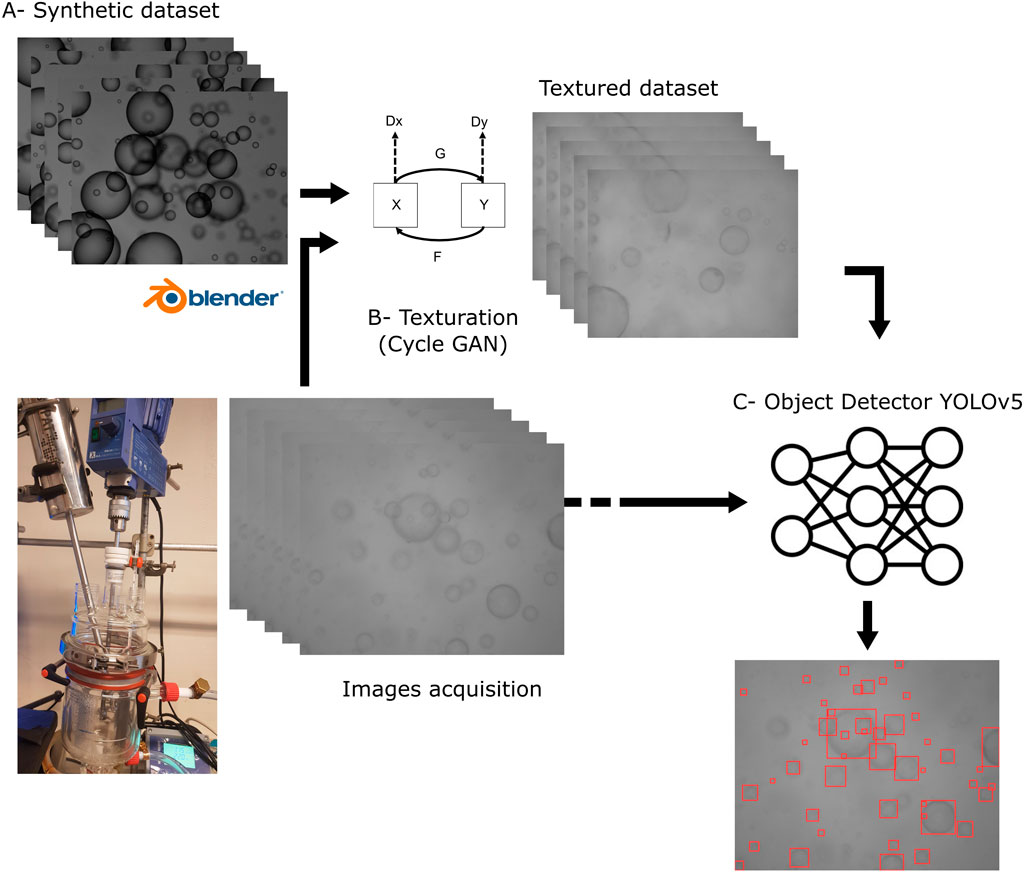
Figure 1. Main flowchart of the proposed algorithm. In this study, experimental images are taken by an endoscopic probe (SOPAT GmbH) immersed in a stirred tank containing a water–oil dispersion generated by agitation.

Allowing these features, the training of such detection networks usually requires a dataset containing several thousand images with labeled objects, which can be a problem. To address this, we took advantage of synthetic images in order to build a large training base of labeled images containing both sharp and blurred droplets. Images were generated from modeling software with 3D rendering: the free and open-source Blender software 3.0.1 Community (2018). The use of synthetic images enables complete control of the distribution of diameters of the spherical objects and ensures that they obey a controlled probability law of size and occurrence in the picture, as required for the training of the CNN. Blender 3.0.1 is set up to create a 3D scene divided into three volumes of equal sizes located in front of a virtual camera. In this way, 3D scenes mimic camera acquisition as closely as possible, with blurred objects in the background, a median zone of sharpness corresponding to the camera’s depth of field, and blurred objects in the foreground. The code randomly positions a user-defined number of spheres in the three volumes. To ensure this randomness, the Blender images were generated using Python scripts. During this process, if two spheres intersect, one is kept and a new position is randomly drawn until a location where this sphere will intersect with no others can be found. In addition, it is possible to adjust the depth of the various volumes, especially Volume 1 to match the depth of field of any optical acquisition system. Finally, the code performs a projection of the 3D spheres in the 2D plane of the virtual camera, possibly taking into account some features of the virtual scene such as the light and optical properties of the objects (refractive index) to produce a “realistic” 2D image (Community, 2018; Hess, 2010), see Figure 2A. The final image, an example of which is shown in Figure 2A, has a size of 1024 × 1280 squared pixels, corresponding to that of the camera used for acquisition. It can be cropped to meet any CNN input requirement.

Figure 2

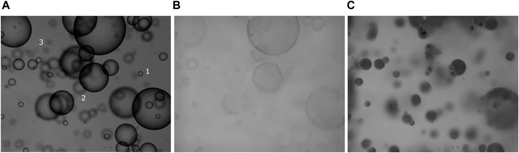
Figure 2. (A) Typical image of droplets relevant for solvent extraction applications produced by Blender software. (B) Results obtained after CycleGan texturing for liquid–liquid system made of transparent fluids. (C) Results obtained after CycleGan texturing for opaque particles dispersed in a transparent continuous phase.

Dividing the measurement volume in three zones allows us to distinguish three families of objects.

$•$ Volume 1: Sharp objects randomly distributed in the focus zone of the virtual camera (cf. mark one in Figure 2A),

$•$ Volume 2: “Blurred” objects randomly distributed outside the focus zone in front of the virtual camera (cf. mark two in Figure 2A),

$•$ Volume 3: “Very blurred” objects randomly distributed in the sub-volume furthest from the camera’s point of view which contribute to the formation of a realistic background in the image (cf. mark three in Figure 2A).

It is therefore possible to use Blender to define the geometric characteristics (3D position in space, diameter) of the droplets located in the focus zone, that is, in the first volume. This allows the generation of a label file containing the dimensions and positions of the annotated bounding boxes for each image. For example, in the case of a sharp droplet with diameter $d$, the corresponding annotated bounding box is centered on the droplet and its dimension is $d\times d$. Thus, only the objects belonging to the first zone are labeled, which then guides the network to detect, after training, only sharp droplets in the real image without having to consider a sharpness metric that is always hard to define. However, despite this zonal partition of space, images produced by Blender might be too coarse and not sufficiently realistic with regards to the experimental images due to factors such as fluid concentration gradients, effective depth of field, and inhomogeneous light intensity. In particular, the texture of the synthetic droplets remains quite unrealistic at this stage, especially for fluid systems with a dark dispersed phase; it thus becomes imperative to use real images in a subsequent stage in order to texture the synthetic droplets created by Blender.

To address this issue and in order to reinforce the learning process, a texture transfer from real to synthetic images was performed using a second network from the GANs family (Goodfellow et al., 2014). This type of network is very useful for transferring texture between images thanks to non-paired data. From two distinct database images of same size, respectively originating from the synthetic images database and a real image database, the network learns the statistical properties of the textures of the real images and applies them to the synthetic images. Conversely, it learns the statistical properties of the textures of the synthetic images, hence its name “CycleGANs” Zhu et al., (2017). In the considered application of droplet detection in multiphase flows, texture transfer is particularly relevant as it allows switching from any fluid system to another, even with colored fluids, by simply changing the texture of the same synthetic image dataset (cf. Figure 2), assuming that the droplet size range remains the same. Moreover, CycleGAN can fine-tune the droplet size distribution of synthetic images to that of real images by adjusting their sharpness during the texture transfer process, resulting in an extremely realistic image dataset with fully known parameters. Consequently, some of the labeled droplets in Volume 1 may become blurred, making them less visible in the resulting image, forcing the YOLO object detector to also learn how to measure them, thereby increasing its performance after training.

Based on the concept of transfer learning, our YOLO network was trained starting from initial weights learned from a MS COCO (Microsoft Common Objects in Context) image dataset (Lin et al., 2015) to benefit from the network’s prior learning. The time required for the different steps and the computing resources used are indicated in Table 1, considering a dataset of 2,000 images. One epoch corresponds to a complete presentation of the training dataset to the algorithm. In this study, two textures were taken into account, one corresponding to transparent fluids and the other to opaque fluids. Thus, the work of training the YOLO network and texturing the dataset was carried out twice and the calculation of the learning base only once.

Table 1

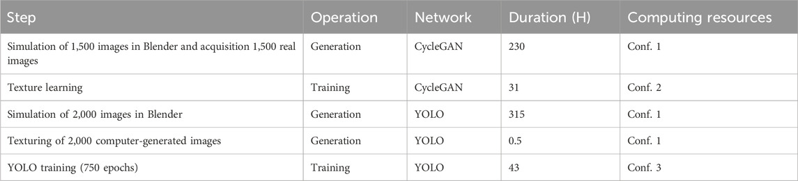
Table 1. Computing resources and time required for the main steps of the method - Conf. 1: 32 AMD Milan processor cores +1 NVIDIA A 100 graphics card 80 GB ram - Conf. 2: 128 AMD Milan processor cores +4 NVIDIA A 100 graphics card 80 GB ram - Conf. 3: 8-core Intel(R) Xeon(R) Gold 6334 CPU @ 3.60 GHz +1 NVIDIA A 100 graphics card 80 GB ram.

3 Performance evaluation by numerical study

The method’s performance was first evaluated by performing a sensitivity study on a test dataset of 1,000 simulated images. Two characteristics affecting the quality of the training were considered: the effect of the texturing and the effect of the dataset size. The efficiency of the proposed methodology is measured in terms of both precision, $P$, and recall, $R$—two common evaluation metrics often used together to assess the overall performance of an object detection model. “High precision” indicates that when the model makes a positive prediction, it is usually correct, while “high recall” indicates that the model is efficient at finding most of the relevant objects in the image. Achieving a good balance between $P$ and $R$ is important, as there is often a trade-off between them.

To calculate these metrics, it is assumed that there is only one class of objects (drops) and that they have been annotated for each image in the test dataset. As specified in Section 2, for each image the network predicts some bounding boxes to which it associates a confidence threshold between 0 and 1. This scalar value may be apprehended as some kind of trust or probability that the predicted bounding box contains an object. Only predicted bounding boxes with a confidence score greater than 0.7 are here considered as positive predictions (PP) and retained for further analysis.

Before defining precision and recall, we need to recall the concept of intersection over union, $(IoU)$, or the “Jaccard index”. $IoU$ is a positive value that evaluates the overlap between the predicted bounding box and the ground truth bounding box of an object. It is calculated as the ratio between the area of intersection and the area of the union of the two bounding boxes. Considering two objects, $O_1$ and $O_2$, $IoU$ can be written as follows:

$IoU=\left|O_1\cap O_2\right|/\left|O_1\cup O_2\right|$

where $\left|O_1\cap O_2\right|$ represents the area of the intersection between the bounding boxes of $O_1$ and $O_2$ and $\left|O_1\cup O_2\right|$ represents the area of the union of the bounding boxes of $O_1$ and $O_2$—the total area covered by the two bounding boxes. The $IoU$ value ranges from 0 to 1, with

$•$ $IoU=0$ indicating that $O_1$ and $O_2$ have no overlap, meaning that they are completely separated.

$•$ $IoU=1$ indicates that $O_1$ and $O_2$ perfectly overlap, meaning that they are identical.

Usually, correct detection or true positive detection, $TP$, is considered when the predicted bounding box has an $IoU$ greater or equal to 0.5 with the corresponding ground truth bounding box.

Precision, $P$, measures the accuracy of the positive predictions made by the model. It quantifies the ratio between $TP$ and the total number of positive predictions, $PP$, and is written as:

$P=\frac{TP}{PP}$

Higher precision indicates fewer false positive predictions and that the model can more correctly identify relevant objects among the predicted positive instances. Here, precision is a measure of how many retrieved droplets are relevant. Note that below a confidence score of 0.7, $P$ decreases drastically, explaining the frequent choice of such a threshold by YOLO users.

Similarly, recall, $R$, measures the ability of a model to identify all relevant objects in the dataset. It quantifies the ratio between true positive detections and the total number of ground truth objects, $I$ and is written as:

$R=\frac{TP}{I}$

A higher recall indicates that the model can identify a larger proportion of actual positive instances, reducing the number of undetected objects (false negatives). In this context, $R$ is a measure of how many relevant drops are retrieved by the model.

Logically, recall and precision are affected by the $IoU$ thresholds. As the $IoU$ threshold increases, requiring a higher degree of overlap between predicted and ground truth bounding boxes, the number of true positive detections decreases, affecting both recall and precision.

The last metric used in this study is $mAP@0.5$, where “mAP” stands for “mean Average Precision”. $mAP@0.5$ is an evaluation metric commonly used to quantify the overall performance of object detection models such as YOLO. It is calculated by first computing the average precision, $AP$, for each class of objects detected by the model at a specific $IoU$ threshold of 0.5 following the next three steps:

$•$ compute precision and recall values by varying the confidence score for the predictions;

$•$ construct a precision–recall curve by plotting precision values against recall values;

$•$ calculate the area under the precision–recall curve $(AP)$ for that specific class.

$mAP$ is therefore the average of the $AP$ scores for all object classes in the dataset, and in the case of a single object class, $AP$ is equal to $mAP$.

3.1 Impact of CycleGAN texturing

The first effect investigated was the impact of the texturing on drop detection performance. For this purpose, a database of 2,000 images was first created and then textured using the CycleGan network with either light or dark textures (based on real images) in order to obtain two additional sets of images. The three datasets of images, no texture, light-textured, and dark-textured, are geometrically identical but exhibit different appearances (Figure 2). Then, the detection network was trained similarly and independently on each of these datasets. In a second step, an additional dataset of 1,000 test images with no texture was generated and textured with both dark and light textures.

The three YOLO networks trained previously were then used to perform detections on each of the two textured test sets. The precision and recall were calculated with a confidence level greater than or equal to 0.95 to only detect those objects considered by YOLO to be droplets with a high level of confidence (Table 2).

Table 2

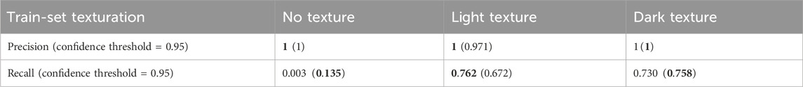
Table 2. Detection metrics calculated on 2 × 1,000 synthetic test images with, respectively, light (no parenthesis) and dark (in parenthesis) textures using three detection algorithms trained on three databases of synthetic images with no, light, and dark textures, respectively. Numbers in bold indicate highest value.

Based on these results, it can be observed that regardless of the texture considered, only a negligible number of detected objects do not correspond to droplets. This is reflected in the precision value, which approach a perfect detection $(R=1)$ in almost all scenarios. The only slightly failing scenario is the detection of dark droplets with a network trained on the light texture database. This is an expected result since there is only one type of object to detect. It follows that the texture of the image database here has little impact on precision.

Conversely, the texture is observed to have a more significant impact on the recall. The neural network trained on non-textured synthetic images achieved nearly zero recall when applied to light textured images and exhibited a low recall on dark textured images. This is because non-textured synthetic images show a greater visual resemblance with dark images than with light ones (cf. Figure 2). In the other two cases, logically, the network trained with the right texture is the one with the best recall, highlighting the substantial impact of image texturing.

In conclusion, the application of CycleGAN for texture transfer has a substantial impact on recall and is fundamental to ensuring correct and efficient object detection.

3.2 Effect of the size of the training database

The network only needs to learn to detect a single class of objects corresponding to the droplets within the measurement volume. Therefore, it should be possible to achieve this learning task with a limited number of images, resulting in reduced training time. To assess the sensitivity of the detection network’s performance on the size of the training database, we conducted several training sessions using image sets of increasing sizes. The study was performed in the case of synthetic images containing a single class of objects to detect, characterize, and simulate droplets. Training datasets of 30, 100, 200, 500, 1,000, and 2,000 images were used, with each image containing around 52 labeled droplets. In each case, the sample images were randomly taken in the same pool of 2,000 synthetic textured images. The training was performed with the same number of epochs (750) and the performance was then assessed from the same test image set using mean average precision at an IoU threshold of 0.5.

Figure 3 shows the evolution of both the $mAP@0.5$ and the training duration as a function of the size of the training dataset. This clearly highlights the substantial improvement of the learning process when the number of images in the training set includes more than 100 images. The training duration logically increases linearly with the number of images. Consequently, we can conclude that the optimal dataset size is around 100 images.

Figure 3

Figure 3. Evolution of the mean average precision mAP@0.5 (in green) and the learning process duration (in purple) with the size of the training database.

Figure 4 provides a more in-depth analysis of the detected droplet count evolution. It illustrates that a minimum of 2,000 training images is required to ensure that the detected proportions of “small” and “large” droplets are representative of the studied population. Indeed, in this case, the network learns to detect small objects only for training datasets larger than 500 images which are, for example, essential in most multiphase flow processes to accurately predict the contact area between the dispersed and continuous phases.

Figure 4

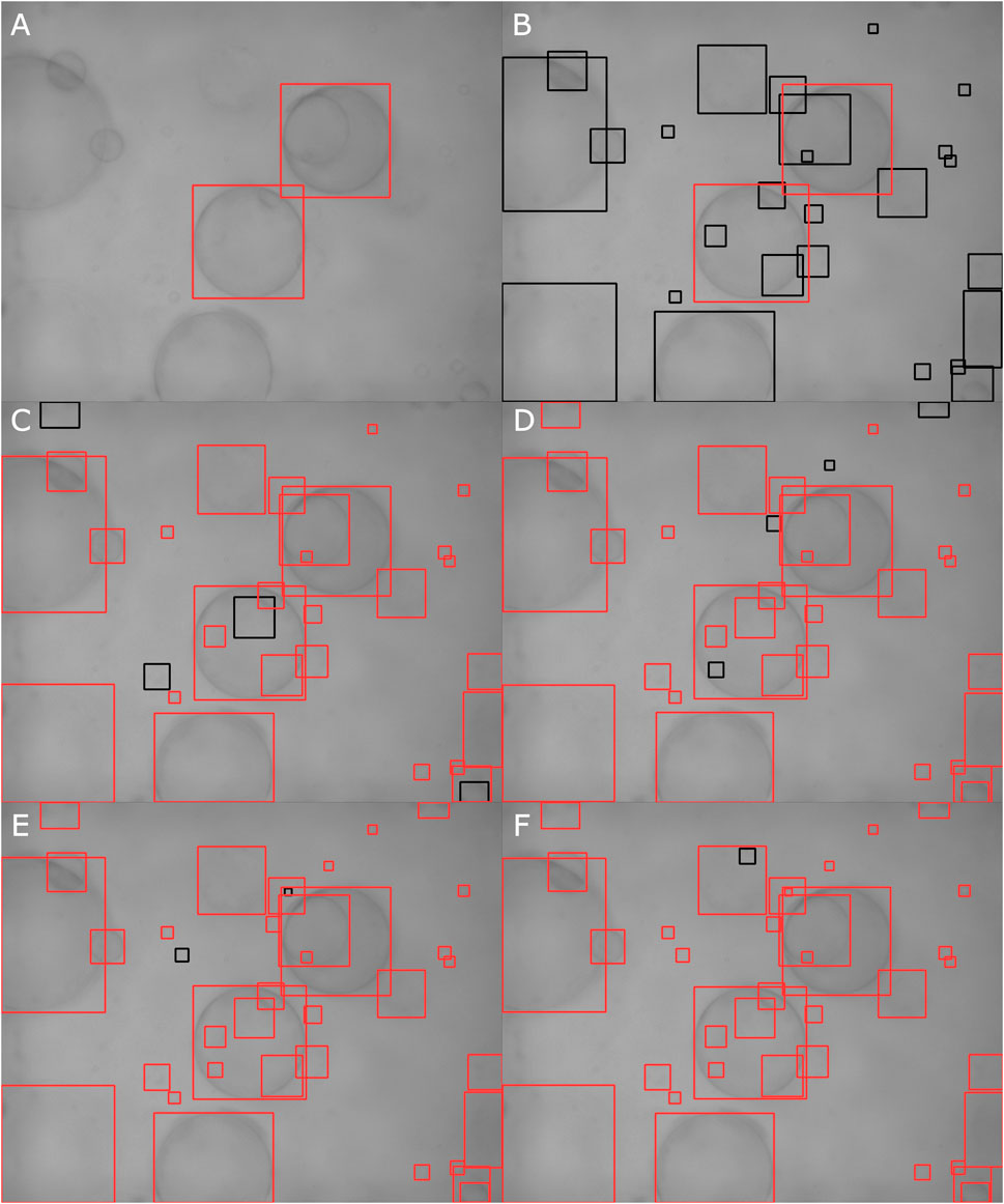
Figure 4. Droplets detected in an image by YOLOv5 trained on (A) 20 images, (B) 100 images, (C) 200 images, (D) 500 images, (E) 1,000 images, or (F) 2,000 images. The red boxes indicate previously detected droplets (i.e., in the smaller database); the black boxes indicate new detections (i.e., thanks to the consecutive increase in the database.).

3.3 Comparison with two deterministic algorithms: the circular Hough transform and a commercial pattern recognition algorithm

To compare the performance of the algorithm with the current state of the art, we implemented a benchmark with the circular Hough transform (CHT) and the SOPAT GmbH algorithm, two widely used circle recognition algorithms. The case study was a set of 1,000 synthetic images with the light texturing of the experimental case studied in Section 4.

The CHT implements the following main steps (Illingworth and Kittler, 1988):

$•$ identifies edges in the image, often using techniques like the canny edge detector;

$•$ creates an accumulator array where edge points vote for potential circle centers and radii based on their spatial relationships;

$•$ accumulates votes to find potential circle parameters with higher votes, indicating possible circles;

$•$ identifies local peaks in the accumulator array, representing potential circle centers and radii;

$•$ retrieves circle parameters from the local maxima and defining the detected circles in the image.

Before applying the CHT, a two-step image processing is performed to improve the contrast of the droplets against the background. It consists of flat histogram equalization followed by noise removal using a trained neural network specialized in blind denoising (Zhang et al., 2023).

In the framework of this paper, the release (V1-4-42) of the SOPAT image processing ensures robust and accurate drop detection by pre-filtering the series of images to remove irrelevant and misleading information. This is achieved by subtracting an integrated sequence. The noise in the pictures is then reduced using the self-quotient image method Gopalan and Jacobs (2010), which normalizes the intensity of every local pixel based on the local environment. This is done by dividing the processed image by a smoothed version of itself. Drop recognition is then achieved through a three-step process: (i) pattern recognition by correlating pre-filtered gradients with search samples; (ii) pre-selecting plausible circle coordinates; (iii) classifying each of those circles through an exact edge examination. The software uses a normalized cross-correlation procedure to evaluate possible drop matches. This automated image analysis algorithm is one of the fastest and most efficient; it overcomes typical limitations of image processing such as circular shape overlapping. More technical details and results about this algorithm can be found in Maaß et al. (2012) and Panckow, Robert P. et al. (2017).

A typical result of three-images processing is presented in Figure 5. For this example, the processing time on a laptop (Intel^® Core™ i7-11850H) is of 48, 5.6, and 2.3 s for the CHT, SOPAT, and BYG-Drop algorithms, respectively. In this case, for a total of 53 annotated drops in the image, CHT detects 19 drops, 13 correct and 6 incorrect, and the commercial algorithm only 15 correct (no incorrect), while BYG-Drop detects 41 correct (no incorrect).

Figure 5

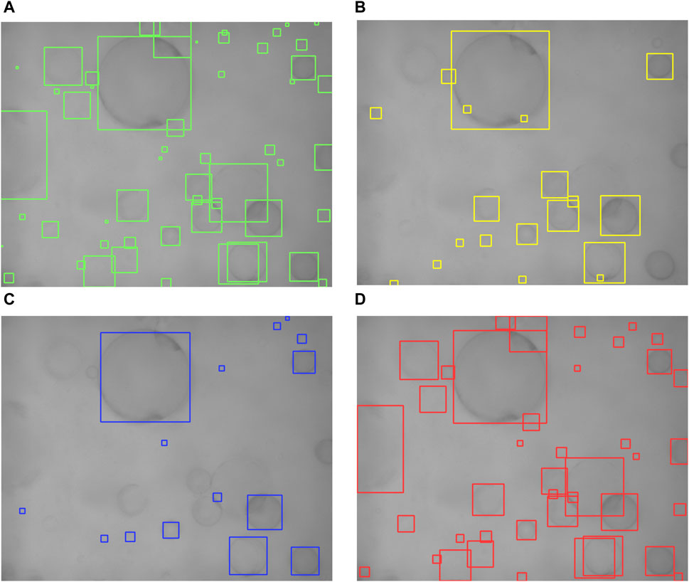
Figure 5. Example of droplet detection results on a synthetic image: (A) Ground truth, (B) CHT, (C) SOPAT algorithm, (D) BYG-Drop.

The results integrated for the entire sequence of 1,000 images are shown in Table 3. Again, with twice the recall of the other two techniques, BYG-Drop detects significantly more relevant droplets. The commercial algorithm maintains high precision, ensuring that only relevant drops are detected. The circular Hough transform fails on both metrics.

Table 3

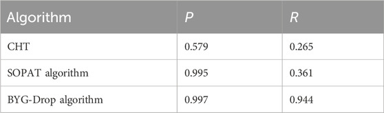
Table 3. Respective detection performance of circular Hough transform, SOPAT algorithm, and BYG-Drop algorithm in terms of precision and recall calculated on a 1,000 synthetic image dataset.

A numerical analysis of the histograms (Figure 6) provides a more detailed analysis of the performance of the different algorithms. Once again, CHT fails to achieve the correct size distribution. The commercial algorithm, on the other hand, finds a distribution consistent with the ground truth but with a much lower number of droplets detected than the ML approach. A bias is also evident in the middle classes, around a size of 100 pixels. The proposed algorithm correctly recovers the distribution of the shape and number of drops, except for the very smallest classes (less than 6 pixels) which is intrinsic to the object detection algorithm used (YOLO-v5) but also corresponds to the detection limit imposed by the optical setup.

Figure 6

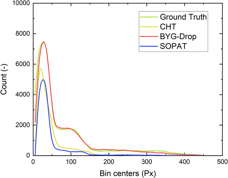
Figure 6. Histograms in numbers of total droplets detected by the three considered algorithms.

4 Benchmark on experimental data

Finally, for comparison purposes on a real test case, an experimental study of the formation of an oil-in-water emulsion was conducted using both an in situ endoscopic probe to record images of the droplets in the dispersion and offline analysis of emulsion samples using a laser diffraction granulometer (Mastersizer 3,000 from Malvern) that directly provides the DSD.

4.1 Material and methods

The fluids used were ultrapure water (viscosity of 1 mPa.${\mathrm{s}}^{-1}$) and silicone oil (viscosity of 200 mPa.${\mathrm{s}}^{-1}$). The mass fraction of oil was 2.5%. Added in the water was 0.3 % wt of Polysorbate 20 (Tween^® 20, Sigma-Aldrich, Germany) to stabilize the emulsion and prevent droplet coalescence during its transport and analysis in the laser granulometer. The experiments were performed at room temperature.

The setup is shown in Figure 7, consisting of a 1-L glass vessel equipped with a 3-blade Mixel TT impeller and 4 baffles to avoid vortex formation. Emulsion formation was achieved by adjusting the amounts of the aqueous and organic phases to give a hold-up of 2.5%. Water and surfactant were first mixed by vigorous stirring at maximum speed, which was then set at 600 rpm, and oil was then added 2 minutes before starting the image acquisitions. The fluids were weighed using a balance from Mettler (PM6000) with a precision of $\pm$0.1 g.

Figure 7

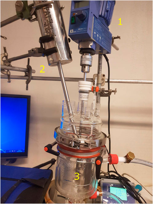
Figure 7. Experimental setup, including, 1- stirrer motor, 2- in situ imaging SOPAT Probe, and 3- stirred tank.

The images were acquired using a commercial endoscopic probe from SOPAT GmbH. The probe was used in reflection mode with a white Teflon reflector and a 6 mm gap. The first image acquisition took place 2 min after adding the oil (to ensure uniformity in the vessel), called $t_0$. A total of 11 acquisition runs of 200 images each, with a frame rate of three images per second, were made. The image acquisitions were spaced 400s apart, leading to a total measurement time of 67 min.

During the course of the experiments, four samples of approximately 75 mL each were taken at $t_0$+400s, $t_0$+1,200s, $t_0$+2,000s, and $t_0$+4,000s, at the end of the experiment.

4.2 Image processing results for oil–water emulsion

The three algorithms described above were applied successively to the 11 sets of images recorded by the endoscopic probe. Here, the detection threshold of YOLO was raised to 0.95 to detect only droplets that perfectly met the sharpness criteria of the training. An example of a raw image is shown in Figure 8A and of the results of droplet detection for CHT, SOPAT, and BYG-Drop in Figures 8B–D, respectively. In this example, which was taken at random out of the 2,200 shots taken, we can clearly see that, despite raising the threshold to 0.95, BYG-Drop is the algorithm that positively detects the highest number of droplets.

Figure 8

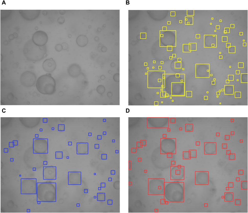
Figure 8. Typical results obtained on a real experimentally acquired image: (A) raw image, (B) detection results with CHT, (C) detection with SOPAT algorithm, and (D) detection with proposed algorithm.

From these detections, an evaluation of the DSD at each time step was constructed. Figure 9 compares the DSD in volume measured with the imaging and laser granulometry techniques at the four time-steps sampled. For both techniques, the evolution of the droplet size distributions is typical of the fragmentation of the oil droplets under agitation. The results of the two techniques are in good agreement, except for the smaller sizes where the number of small droplets measured by the granulometer is higher than by image processing. This is partly due to the limited resolution of the images taken by the endoscopic probe, which makes the smallest objects undetectable and also due to the laser diffraction, which tends to overestimate the fraction of small droplets as they remain in the measurement sample for longer periods than the bigger ones because of their lower velocity (Kowalenko and Babuin, 2013; Sijs et al., 2021).

Figure 9

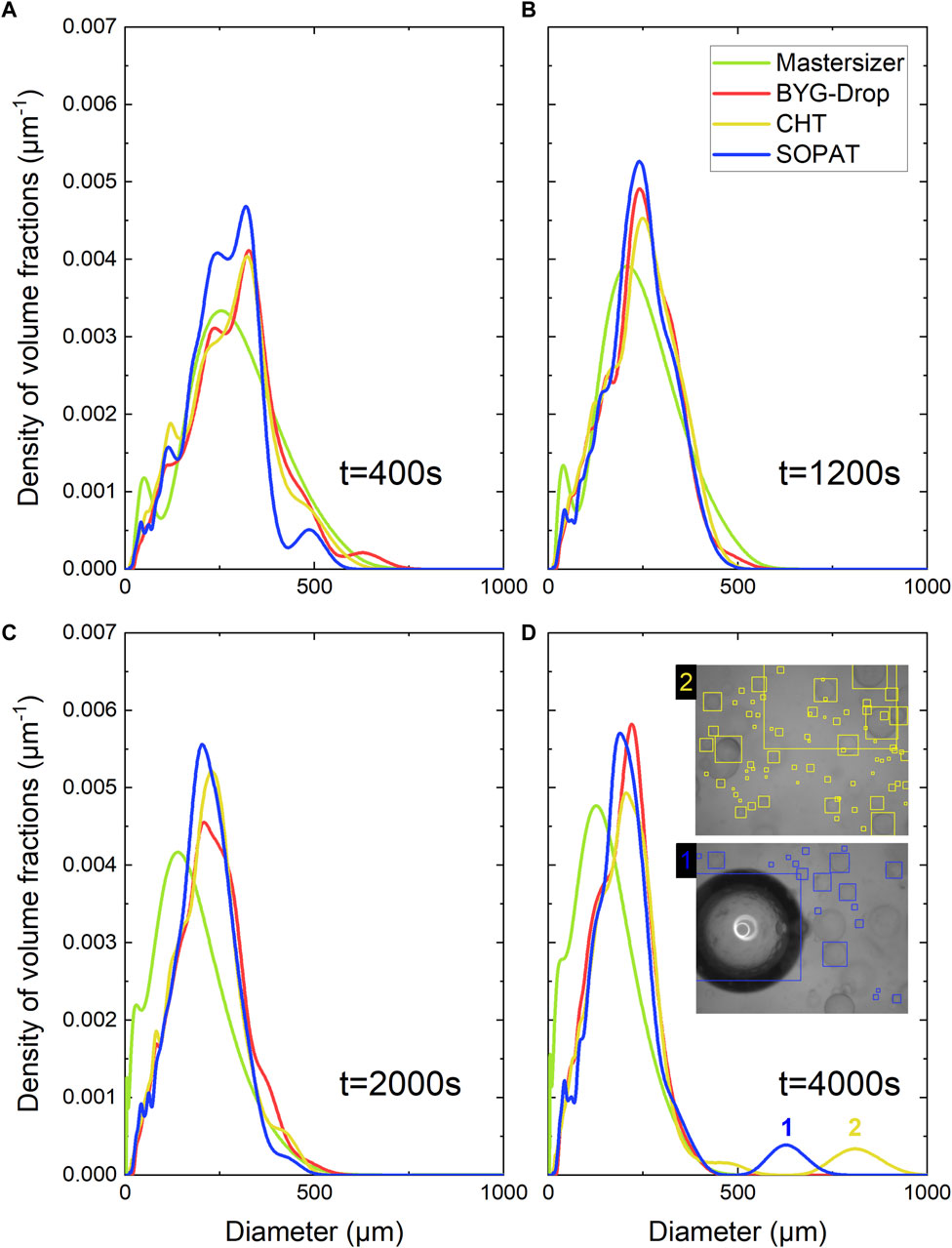
Figure 9. DSD retrieved from laser diffraction granulometer and the three different image processing at (A) $t_0$+400s, (B) $t_0$+1,200s, (C) at $t_0$+2,000s, and (D) $t_0$+4,000s.

The distributions for the different image processing techniques appear similar (cf. Figure 9), partly thanks to normalization induced by the volume density presentation. However, once again, the machine learning approach detects a significantly higher number of droplets despite the increase in the decision threshold, making the results statistically more reliable. In addition, the other two algorithms sometimes make detection mistakes, such as detecting ghost droplets with CHT (see two in Figure 9D) or taking account of air bubbles with the commercial algorithm (see one in Figure 9D), which can bias the tails of the size distributions.

Finally, the robustness and the efficiency of the new method for detecting droplets with a different texture (by image coloration) was evaluated with the same two fluids by adding a dye (methyl blue at 1 mg/L) in the dispersed phase. This addition makes it possible to obtain a dark dispersed phase without altering the emulsification properties, allowing reuse of the experimental setting described in Section 4.1. For this second experiment, 95 acquisition runs of 15 images each, with a frame rate of 10 images per second and trigger interval of 1.5 s were taken, corresponding to a total acquisition time of 285 s.

YOLO was trained on the same database of synthetic images but textured darkly. The algorithm was then applied on the full data set of 1,425 images with a confidence threshold of 0.95. For comparison purposes, the same sequence was processed with CHT, which is highly effective for images with such high contrast.

Figure 10A shows a typical image, while Figure 10B compares the count histograms measured with the two algorithms. The machine learning approach again detects a significantly higher number of droplets, especially for the smallest classes, making the results statistically more reliable. These experiments confirm both the ability of the combined algorithm to detect a wide spectrum of textures and the powerful aspect of texturing.

Figure 10

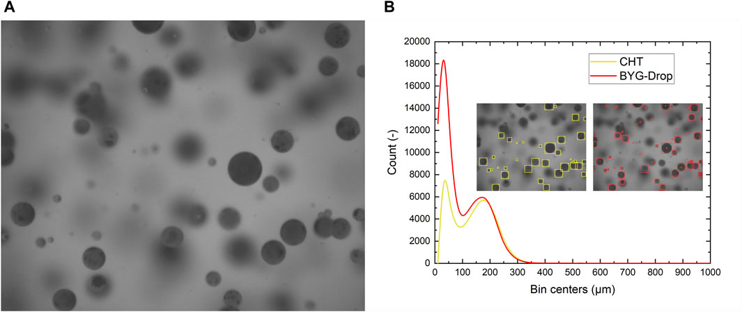
Figure 10. (A) Typical acquisition of fluids with a dark dispersed phase. (B) Histograms in numbers of total droplets detected by CHT and BYG-Drop.

5 Conclusion

A new image processing machine learning algorithm for droplets detection in liquid–liquid systems, BYG-Drop, is here introduced. It is based on the combination of three numerical tools: the object detector YOLOv5, the free and open-source 3D computer graphics software Blender, and a neural network specialized in texture transfer, CycleGAN. This method surpasses the usual image processing techniques on digital test cases both in terms of precision and in the droplet numbers detected, as demonstrated by a recall almost twice as high as the best other algorithms. These promising results are confirmed when processing experimental images, for which the machine learning processing remains consistent with the usual techniques, whether laser diffraction or other image processing, while performing better in terms of the number of good detections in each image.

Using synthetic images for training instead of manually labeled real images has several advantages, including the ability to effortlessly label a large dataset, which turns out to be an enormous advantage for efficient learning. As a result, the trained network can easily avoid false detections such as ghost drops or air bubbles.

Moreover, CycleGAN image texturing allows easy and fast adaptation to different fluid systems (colored and transparent, droplet size, shape, etc.). This makes droplet size measurement by imaging and image processing an even more versatile and adaptable in situ technique.

Finally, the processing time for each image is faster, which is an advantage of YOLO, a network designed for real-time video detection. Although YOLO version 5 has been trained here for a posteriori processing, we are confident that BYG-Drop can perform real-time DSD measurement in chemical processes using a more advanced version of the object detector and GPU implementation Wang et al. (2023).

Data availability statement

The raw data supporting the conclusions of this article will be made available by the authors without undue reservation. The network weights trained on both dark and light datasets are available on the following Github repository: https://github.com/banag0/BYGDrop.

Author contributions

GB: Conceptualization, Data curation, Methodology, Writing–original draft. FL: Conceptualization, Methodology, Validation, Writing–original draft, Writing–review and editing. SC: Validation, Writing–review and editing. TR: Conceptualization, Methodology, Validation, Writing–review and editing. DL: Validation, Writing–review and editing. NS-O: Validation, Writing–review and editing.

Funding

The authors declare that financial support was received for the research, authorship, and/or publication of this article. This work was supported by the CEA Energy Division (SIACY project). SC and FL are carrying out part of this work within the framework of the priority research program and equipment on recycling, recyclability, and re-use of materials.

Conflict of interest

The authors declare that the research was conducted in the absence of any commercial or financial relationships that could be construed as a potential conflict of interest.

Publisher’s note

All claims expressed in this article are solely those of the authors and do not necessarily represent those of their affiliated organizations, or those of the publisher, the editors and the reviewers. Any product that may be evaluated in this article, or claim that may be made by its manufacturer, is not guaranteed or endorsed by the publisher.

Abbreviations

$AP$, average precision; $CHT$, circular Hough transform; $CNN$, convolutional neural network; $DSD$, droplet size distributions; $GAN$, generative adversarial network; $GPU$, graphics processing unit; $I$, number of ground truth objects; $IoU$, intersection over union; $mAP$, mean average precision; $ML$, machine learning; $MSCOCO$, Microsoft Common Objects in Context; $P$, precision; $PP$, number of positive predictions; $R$, recall; $RCNN$, region-based convolutional neural network; $TP$, true positive detections; $YOLO$, you only look once.

References

Beucher, S., and Meyer, F. (2019). The morphological approach to segmentation: the watershed transformation.

Google Scholar

Bian, Y., Dong, F., Zhang, W., Wang, H., Tan, C., and Zhang, Z. (2013). 3D reconstruction of single rising bubble in water using digital image processing and characteristic matrix. Particuology 11, 170–183. doi:10.1016/j.partic.2012.07.005

CrossRef Full Text | Google Scholar

Clift, R., and Grace, W. M. (1999). Bubbles, drops and Particles, 1978, 10. New York. Academic Press.

Google Scholar

Community, B. O. (2018). Blender - a 3D modelling and rendering package. Amsterdam: Stichting Blender Foundation. Blender Foundation.

Google Scholar

Cui, Y., Li, C., Zhang, W., Ning, X., Shi, X., Gao, J., et al. (2022). A deep learning-based image processing method for bubble detection, segmentation, and shape reconstruction in high gas holdup sub-millimeter bubbly flows. Chem. Eng. J. 449, 137859. doi:10.1016/j.cej.2022.137859

CrossRef Full Text | Google Scholar

de Cerqueira, R. F., Perissinotto, R. M., Verde, W. M., Biazussi, J. L., de Castro, M. S., and Bannwart, A. C. (2023). Development and assessment of a particle tracking velocimetry (PTV) measurement technique for the experimental investigation of oil drops behaviour in dispersed oil–water two-phase flow within a centrifugal pump impeller. Int. J. Multiph. Flow 159, 104302. doi:10.1016/j.ijmultiphaseflow.2022.104302

CrossRef Full Text | Google Scholar

De Langlard, M., Al Saddik, H., Lamadie, F., Charton, S., and Debayle, J. (2017). “A multiscale method for shape recognition of overlapping elliptical particles,” in Proceedings - international conference on pattern recognition.

Google Scholar

Diwan, T., Anirudh, G., and Tembhurne, J. V. (2023). Object detection using YOLO: challenges, architectural successors, datasets and applications. Multimedia Tools Appl. 82, 9243–9275. doi:10.1007/s11042-022-13644-y

CrossRef Full Text | Google Scholar

Emmerich, J., Tang, Q., Wang, Y., Neubauer, P., Junne, S., and Maaß, S. (2019). Optical inline analysis and monitoring of particle size and shape distributions for multiple applications: scientific and industrial relevance 27.

Google Scholar

Fu, Y., and Liu, Y. (2019). BubGAN: bubble generative adversarial networks for synthesizing realistic bubbly flow images. Chem. Eng. Sci. 204, 35–47. doi:10.1016/j.ces.2019.04.004

CrossRef Full Text | Google Scholar

Goodfellow, I., Pouget-Abadie, J., Mirza, M., Xu, B., Warde-Farley, D., Ozair, S., et al. (2014). “Generative adversarial nets,” in Advances in neural information processing systems, 2672–2680.

Google Scholar

Gopalan, R., and Jacobs, D. (2010). Comparing and combining lighting insensitive approaches for face recognition. Comput. Vis. Image Underst. 114, 135–145. doi:10.1016/j.cviu.2009.07.005

CrossRef Full Text | Google Scholar

Haas, T., Schubert, C., Eickhoff, M., and Pfeifer, H. (2020). BubCNN: bubble detection using Faster RCNN and shape regression network. Chem. Eng. Sci. 216, 115467. doi:10.1016/j.ces.2019.115467

CrossRef Full Text | Google Scholar

Hess, R. (2010). Blender foundations: the essential guide to learning blender 2.6. (Focal Press).

Google Scholar

Honkanen, M., Saarenrinne, P., Stoor, T., and Niinimäki, J. (2005). Recognition of highly overlapping ellipse-like bubble images. Meas. Sci. Technol. 16, 1760–1770. doi:10.1088/0957-0233/16/9/007

CrossRef Full Text | Google Scholar

Hough, P. V. C. (1962). A method and means for recognition complex patterns. US Patent. US Patent: US3069654A.

Google Scholar

Illingworth, J., and Kittler, J. (1988). “A survey of the hough transform,” in Computer vision, graphics and image processing 44.

CrossRef Full Text | Google Scholar

Ilonen, J., Juránek, R., Eerola, T., Lensu, L., Dubská, M., Zemčík, P., et al. (2018). Comparison of bubble detectors and size distribution estimators. Pattern Recognit. Lett. 101, 60–66. doi:10.1016/j.patrec.2017.11.014

CrossRef Full Text | Google Scholar

Jiang, P., Ergu, D., Liu, F., Cai, Y., and Ma, B. (2022). A review of yolo algorithm developments. Procedia Comput. Sci. 199, 1066–1073. doi:10.1016/j.procs.2022.01.135

CrossRef Full Text | Google Scholar

Jocher, G. (2020). Yolov5 by ultralytics. doi:10.5281/zenodo.3908559

CrossRef Full Text | Google Scholar

Khalil, A., Puel, F., Chevalier, Y., Galvan, J. M., Rivoire, A., and Klein, J. P. (2010). Study of droplet size distribution during an emulsification process using in situ video probe coupled with an automatic image analysis. Chem. Eng. J. 165, 946–957. doi:10.1016/j.cej.2010.10.031

CrossRef Full Text | Google Scholar

Kim, Y., and Park, H. (2021). Deep learning-based automated and universal bubble detection and mask extraction in complex two-phase flows. Sci. Rep. 11, 8940. doi:10.1038/s41598-021-88334-0

PubMed Abstract | CrossRef Full Text | Google Scholar

Kowalenko, C., and Babuin, D. (2013). Inherent factors limiting the use of laser diffraction for determining particle size distributions of soil and related samples. Geoderma 193-194, 22–28. doi:10.1016/j.geoderma.2012.09.006

CrossRef Full Text | Google Scholar

Lin, T.-Y., Maire, M., Belongie, S., Bourdev, L., Girshick, R., Hays, J., et al. (2015). Microsoft coco: common objects in context.

Google Scholar

Maaß, S., Rojahn, J., Hänsch, R., and Kraume, M. (2012). Automated drop detection using image analysis for online particle size monitoring in multiphase systems. Comput. Chem. Eng. 45, 27–37. doi:10.1016/j.compchemeng.2012.05.014

CrossRef Full Text | Google Scholar

Neuendorf, L., Hammal, Z., Fricke, A., and Kockmann, N. (2023). Ai-based supervision for a stirred extraction column assisted with population balance-based simulation. Chem. Ing. Tech. 95, 1134–1145. doi:10.1002/cite.202200241

CrossRef Full Text | Google Scholar

Panckow, R. P., Reinecke, L., Cuellar, M. C., and Maaß, S. (2017). Photo-optical in-situ measurement of drop size distributions: applications in research and industry. Oil Gas. Sci. Technol. †Rev. IFP Energies Nouv. 72, 14. doi:10.2516/ogst/2017009

CrossRef Full Text | Google Scholar

Patil, A., Sægrov, B., and Panjwani, B. (2022). Advanced deep learning for dynamic emulsion stability measurement. Comput. Chem. Eng. 157, 107614. doi:10.1016/j.compchemeng.2021.107614

CrossRef Full Text | Google Scholar

Pieloth, D., Rodeck, M., Schaldach, G., and Thommes, M. (2023). Categorization of sprays by image analysis with convolutional neuronal networks. Chem. Eng. Technol. 46, 264–269. doi:10.1002/ceat.202200356

CrossRef Full Text | Google Scholar

Roehl, S., Hohl, L., Kempin, M., Enders, F., Jurtz, N., and Kraume, M. (2019). Influence of different silica nanoparticles on drop size distributions in agitated liquid-liquid systems. Chem. Ing. Tech. 91, 1640–1655. doi:10.1002/cite.201900049

CrossRef Full Text | Google Scholar

Sijs, R., Kooij, S., Holterman, H. J., van de Zande, J., and Bonn, D. (2021). Drop size measurement techniques for sprays: comparison of image analysis, phase Doppler particle analysis, and laser diffraction. AIP Adv. 11, 015315. doi:10.1063/5.0018667

CrossRef Full Text | Google Scholar

Soille, P. (2004). Morphological image analysis: principles and applications.

Google Scholar

Treybal, F. E. (1980). Mass-transfer operations. 3 edn. McGraw-Hill chemical engineering series.

Google Scholar

Wang, C., Bochkovskiy, A., and Liao, H. (2023). “Yolov7: trainable bag-of-freebies sets new state-of-the-art for real-time object detectors,” in 2023 IEEE/CVF conference on computer vision and pattern recognition (CVPR) (Los Alamitos, CA, USA: IEEE Computer Society), 7464–7475.

CrossRef Full Text | Google Scholar

Yonghong, X., and Qiang, J. (2002). “A new efficient ellipse detection method,” in Proceedings - international conference on pattern recognition, 16.

Google Scholar

Zhang, K., Li, Y., Liang, J., Cao, J., Zhang, Y., Tang, H., et al. (2023). Practical blind image denoising via swin-conv-unet and data synthesis. Mach. Intell. Res. 20, 822–836. doi:10.1007/s11633-023-1466-0

CrossRef Full Text | Google Scholar

Zhang, W. H., Jiang, X., and Liu, Y. M. (2012). A method for recognizing overlapping elliptical bubbles in bubble image. Pattern Recognit. Lett. 33, 1543–1548. doi:10.1016/j.patrec.2012.03.027

CrossRef Full Text | Google Scholar

Zhu, J.-Y., Park, T., Isola, P., and Efros, A. A. (2017). “Unpaired image-to-image translation using cycle-consistent adversarial networks,” in 2017 IEEE international conference on computer vision (ICCV).

CrossRef Full Text | Google Scholar