2D simulation of temperature distribution within large-scale PEM electrolysis stack based on thermal conductivity measurements

Polymer electrolyte membrane electrolyser cells (PEMEC) are recognized as highly suitable for large-scale green hydrogen production from variable renewable sources. To enhance production rates in PEMECs, current densities have gradually increased, resulting in elevated heat generation within the electrolysis cells. Consequently, the consideration of thermal gradients within individual cells within the stacks becomes increasingly crucial. This study presents a 2D thermal numerical steady-state model of an industrial-sized PEMEC stack, predicting thermal gradients within the cells in both stacking direction and along the channels of the flow fields. Through-plane thermal conductivities were measured ex-situ for the titanium felt porous transport layer (PTL), Tion5-W PFSA membrane, and PEMEC catalyst layers (CLs). At a compaction pressure of 16 bar, the wet PTL exhibited a thermal conductivity of 2.7 ± 0.2 W m⁻¹ K⁻¹, the wet membrane of 0.31 ± 0.01 W m⁻¹ K⁻¹, and the wet CLs of 0.19 ± 0.03 W m⁻¹ K⁻¹. When modelled, thermal gradients of 16.5 ± 0.6 K in parallel flow and 17.6 ± 0.5 K in counter-flow were predicted within cells with a 1 m² cell area, operating at 2 A cm⁻². The counter-flow arrangement demonstrated a 0.2% advantage in voltage efficiency. An increase in current density to 3 A cm⁻² resulted in a 10 K rise in thermal differences in both parallel and counter-flow conditions. However, the use of a sintered PTL reduced thermal gradients by approximately 3.7 K at 2 A cm⁻². The simulation indicated a 20%–40% increase in maximal thermal gradients within the stack compared to models using lumped properties within the cells, emphasizing the significance of considering in-cell thermal gradients at the stack level.

1 Introduction

Transitioning away from a fossil-fuel-dependent economy necessitates the exploration of alternative strategies for storing substantial amounts of energy and substituting fossil-based chemicals with renewable-source-based materials. In this context, green hydrogen, derived from renewable energy sources and water, emerges as a pivotal energy carrier (Kavadias et al., 2018; Schiebahn et al., 2015). Among various technologies, polymer electrolyte membrane (PEM) stands out as particularly well-suited for large-scale hydrogen production from fluctuating renewable sources due to its rapid response to load profile changes, high current densities, low operating temperatures, and the superior purity of generated gases (Kumar and Lim, 2022). Notably, recent industrial-scale implementations of PEM electrolysis stacks mark a significant step forward (Zhang et al., 2022). However, to enhance efficiency in terms of hydrogen production per membrane area and consequently reduce production costs, the anticipated rise in current densities is expected to escalate over time (Kumar and Lim, 2022). This heightened current density leads to an augmented production of irreversible heat within the electrolysis stack, posing challenges for heat management as well as degradation control.

In the stacked electrolysis cells (ECs), heat is generated within the membrane electrode assemblies (MEAs) situated at the core of the cells. This heat must then be conveyed through the adjoining porous transport layers (PTLs) to the flow fields (FFs), where water, oxygen, and hydrogen absorb the excess heat produced during the electrolysis process. The heightened production rate of heat results in increased thermal gradients within the ECs, significantly influencing local degradation rates and potentially surpassing the maximum operating temperatures of the PEM (Burheim, O. S., 2017; Krenz et al., 2023). Consequently, with increasing current densities, it becomes imperative to consider thermal gradients and temperature distribution within the cells of polymer electrolyte membrane electrolysis cell (PEMEC) stacks for efficient management and cell design.

The thermal conductivities of materials employed in various layers of PEM fuel cells have been extensively studied in existing literature. Nafion^® membrane conductivity has been investigated in previous works (Ahadi et al., 2016; Asmatulu et al., 2018; Burheim et al., 2010; Khandelwal and Mench, 2006), while the thermal conductivity of catalyst layers (CLs) with diverse compositions has been explored in (Ahadi et al., 2017; Bock et al., 2020a; Burheim et al., 2014; Khandelwal and Mench, 2006). Materials associated with PTLs, with and without micro porous layers, have been measured in (Bock et al., 2019; 2018; Burheim et al., 2015; 2013; Burheim and Pharoah, 2017; Khandelwal and Mench, 2006).

As stated, most existing models in the literature assume a constant temperature across the stack when analyzing thermal behavior (Bock et al., 2020b; Nafchi et al., 2022; Yasutake et al., 2022). Few models for a single EC consider thermal gradients in the stacking direction, with the work by Bock et al. marking a pioneering effort in this direction in 2020 (Bock et al., 2020b). Predicting temperature gradients within the EC requires precise knowledge of the thermal conductivities of the materials used in the cells. Although some studies have measured the thermal conductivity of certain components, comprehensive models using exact, measured thermal conductivities for all layers inside the EC are lacking in the literature.

Contrastingly, investigations into the thermal properties of materials used in PEMECs have been limited. Although the thermal conductivity of Nafion^® membranes can be extrapolated from prior studies, CLs and PTLs exhibit different compositions in fuel cells and electrolysis cells, necessitating separate investigations (Chen et al., 2019; Yuan et al., 2022; Zhao et al., 2023). Bock et al. (2020b) explored the thermal conductivity of various sintered titanium PTLs under varying compaction pressure and humidification levels, while Schuler et al. (2019) conducted in-situ measurements of the thermal conductivity of titanium felt PTLs with different porosities using indirect membrane temperature measurements. However, the thermal conductivity of EC CLs remains unexplored, and existing literature often approximates CL thermal conductivities using values measured in fuel cell CLs, or bulk thermal conductivities (Bock et al., 2020b; Yasutake et al., 2022).

While in-situ measurements under actual electrolysis conditions provide valuable insights, challenges arise due to the need for precise knowledge of distances between thermocouples, influenced by layer compaction and changes in local pressure during thermocouple insertion. Additionally, thermocouple insertion may affect overpotentials and current density distribution within the cell, leading to limited certainty in determined thermal conductivities (Burheim, O. S., 2017). As an alternative, ex-situ methods, such as the laser flash technique, are often employed. However, the porous nature of materials in PEMECs hinders the applicability of this technique, and its effectiveness is compromised when dealing with wetted materials. Hence, the heat flux method, an ex-situ approach measuring temperature drop over a material sample between two pistons under known heat flux, was employed in this study. This method ensures high-precision measurements at different compaction pressures, covering thermal conductivities of both dry and wet EC membrane, CL, and PTL. The apparatus used in this study has been validated in previous works (Bock et al., 2016; Burheim et al., 2010; 2011) and is detailed in the subsequent sections.

This study aims to address the gap of stack-versus cell-level, and lack of PEMEC component thermal conductivity values, by simulating the temperature distribution within an industrial-sized PEMEC stack, considering thermal gradients within the single cells of the stack, and employing measured thermal conductivity values for all layers of the ECs. To achieve this, the study involves the ex-situ measurement of trough-plane thermal conductivities for various components, including platinum-coated titanium felt PTL, Tion5-W PFSA membrane, and mean values of iridium ruthenium oxide anodic catalyst layer (ACL) and platinum black cathodic catalyst layer (CCL). These measurements are conducted under different compaction pressures and humidification levels using the heat flux method. Subsequently, a numerical steady-state thermal model is developed for the industrial-sized PEMEC stack, considering thermal gradients along the channels of the FF and within, as well as between, the single ECs in the stacking direction. The study explores different arrangements, such as parallel and counter-flow, and investigates the impact of various factors, including different PTLs, current densities, and dissimilar inlet temperatures of anodic and cathodic fluids. Furthermore, the study analyzes the influence of water drag through the membrane on temperature gradients and efficiencies within the cells of the stack.

2 Methodology and model development

2.1 Measuring thermal conductivities

2.1.1 Experimental setup

In this study, the thermal conductivities were measured through an ex-situ approach utilizing the heat flux method (Supplementary Figure S1). The experimental setup comprises two steel pistons with a diameter of (21.0 ± 0.1) mm, featuring thin aluminum sleeves at the contact surfaces. The upper piston was heated to approximately 35°C at the top, while the lower piston was cooled to around 10°C at the bottom, achieved through temperature-controlled water circuits. This design ensured that the aluminum sleeves remained close to ambient temperature, thereby minimizing heat exchange with the surroundings. Furthermore, both pistons were thermally insulated against the ambient environment to further reduce heat exchange.

Each piston incorporated three type k thermocouples in the steel section (T1 − T3 and T6 − T8) at a specified distance ($∆x_{tc}$) of 17.70 ± 0.25 mm, exhibiting an accuracy of ±0.05 K. These thermocouples facilitated the measurement of thermal gradients (∆T) over the pistons, enabling the determination of heat flux ($\dot{q}$) in each piston using the known thermal conductivity of steel, denoted as κ_steel, and applying Fourier’s law of heat conduction. The heat flux through the aluminum sleeves (${\dot{q}}_{sample}$) was assumed to be the mean of the heat fluxes through the pistons, as per Equation 1.

${\dot{q}}_{sample}=\frac{{\kappa }_{steel}}{2}\left(\frac{{∆T}_{1-3}}{2∆x_{tc}}+\frac{{∆T}_{6-8}}{2∆x_{tc}}\right)(1)$

A circular sample with a diameter of 21 mm was introduced between the two aluminum sleeves, and the thermal gradient was assessed using two additional thermocouples (T4, T5). These thermocouples were positioned between the aluminum sleeves and the steel pistons. Given the high thermal conductivity of aluminum, it is reasonable to consider it as isothermal. Consequently, the determined thermal gradient can be ascribed to the thermal resistance of the sample, denoted as $R$, and the contact resistances ($\left.R_c\right)$ between the sample and the aluminum sleeves on both sides Equation 2.

$R_{total}=\frac{T_4-T_5}{{\dot{q}}_{sample}}=R+2R_c(2)$

To discern the contact resistance from the bulk resistance, measurements were conducted on samples of varying thicknesses ($\delta$). The sample thickness was initially measured outside the apparatus at a compaction pressure of 0 bar, using an electronic micrometer with a resolution of 1 µm. Subsequently, continuous measurements were carried out within the apparatus under different pressures, utilizing two electronic gauges (Mitutoyo Digimatic Indicator ID-C Series 543), both providing a resolution of 1 µm. The intercept on the axis characterizes the total contact resistance ($2R_c$), while the inverse of the slope corresponds to the bulk thermal conductivity (κ) of the sample. To explore the thermal resistances and compression behavior of the samples under various compaction pressures, a pneumatic piston was employed to apply controlled compaction pressures up to 16 bar on the steel pistons. The applied pressure during measurement of the thermal resistances of the samples is assumed not alter the contact resistance due to the samples being saturated in water (Shum et al., 2017).

2.1.2 Measurement procedure

Before commencing the measurements, the experimental setup underwent calibration using Polyether Ether Ketone (PEEK) samples with a known thermal conductivity value of κ = 0.25 W m⁻¹ K (Van der Vegt and Govaert, 2003), spanning different thicknesses ranging from 0.5 to 1.5 mm. The measurement protocol was consistently applied to each material, involving the following procedure.

Initially, a calibration of the digital gauges was conducted by implementing all required pressure steps without a sample. This step aimed to exclude any potential compaction of the rig due to the applied pressure. Subsequently, samples of four different thicknesses were measured, followed by another calibration without a sample. Each calibration and measurement were carried out at three distinct pressures in an ascending order. The applied pressures varied between materials, with details summarized in Table 1. For dry materials, the first pressure was sustained for 20 min, while the second and third pressures were maintained for 15 min each. Measurements were specifically performed during the last 5 minutes of each pressure step to ensure the formation of stable temperature gradients. The temperatures, pressures, and gauge readings were recorded every 0.1 s. Following the measurement at the highest pressure, the pressure was subsequently reduced to the lowest pressure, and the thickness was measured again to explore potential hysteresis effects. As no significant temperature fluctuations were measured during this step, the pressure was held for 6 minutes.

Table 1

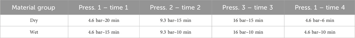
Table 1. Pressure steps for the conductivity measurements.

For wet measurements, Parafilm^® was used to seal the pistons around the aluminium section, minimizing drying of the sample. The impact of Parafilm^® on the measurements was assessed during calibration. Additionally, the holding time at each pressure step was reduced by 5 minutes compared to dry measurements to further mitigate drying. However, the last pressure step was held for 10 min, exceeding the duration in dry materials. A thermal conductivity measurement was incorporated during this step, concurrent with the thickness measurement, to evaluate the influence of drying during the measurements on thermal conductivity.

A PEMEC MEA from FuelCellStore, comprising a Tion5-W PFSA membrane, an iridium ruthenium oxide anode, and a platinum black cathode, each with a loading of 3 mg cm⁻², was employed to approximate the thermal conductivity of the CLs.

The thermal conductivity and compressibility of the membrane were determined in a separate measurement using pure samples of the same membrane with a thickness of 127 µm. This information was subtracted from the MEA measurements to ascertain the CL properties. The contact resistance between the CL and the membrane, as well as between the CLs of the adjacent samples, was assumed negligible, considering the availability of materials in a single thickness, necessitating the stacking of multiple samples to create samples of varying thicknesses. The EC materials were measured in their delivered state, as no aged samples were accessible.

Electrolysers typically operate under compaction pressures of approximately 20–30 bar (Borgardt et al., 2019). Given this, the maximum pressure evaluated during the measurements was set to the maximum pressure capacity of the rig, which is 16 bar. The examined pressures were 4.6, 9.3, and 16 bar.

For the wet measurements, the membrane underwent humidification by immersing the samples in purified water for 1 hour, followed by the removal of excess water using a paper towel. Additionally, the MEA was subjected to a vacuum while soaking in purified water for an hour to facilitate water penetration into the hydrophobic structures of the CLs. To quantify the water content in the samples, their weights were recorded before and after the thermal conductivity measurements, as well as after overnight drying.

As previously mentioned, the thermal conductivity of sintered titanium PTL has been measured ex-situ by Bock et al. (2020b) using the heat flux method. However, titanium felt PTL, another commonly used type of PTL in PEMECs, has only been studied in-situ by Schuler et al. (2019), and never under controlled ex-situ conditions. Therefore, a platinized titanium fibre felt EC PTL (Fuel Cell Store, SKU: 592796-2), with a thickness of 250 μm, was measured both in dry and wet states using the same procedure as before.

During wet thermal conductivity measurements, two mechanisms could lead to drying of the samples. Firstly, water may be forced out of the sample through compaction pressure, resulting in a compressed sample containing less water than an uncompressed one. This phenomenon is anticipated in an EC stack when compaction pressure is applied. Secondly, water may evaporate or flow out of the sample due to inadequate sealing. This effect does not occur in EC operation, as water is continuously fed into the stack. The impact of the second mechanism on the measurement results must be minimized and controlled to ensure measurement accuracy. Due to the apparent high drying in the EC materials, all electrolysis materials were measured via two methods. Initially, by humidifying the sample only before the first pressure step. Subsequently, a second set of measurements was conducted by removing the samples from the apparatus and re-humidifying them between each pressure step. With re-humidification, each pressure was maintained for 15 min, with the last 5 minutes allocated for measurements. The results of the two methods were then compared to determine the impact of drying due to the second mechanism, which is expected to be lower when re-humidifying the samples. Compressibility was only determined from the measurements without re-humidification, as the re-humidification process increased the uncertainty of the compression measurements, given that the samples had to be re-inserted into the apparatus between pressure steps.

2.2 Simulating temperature distribution within a PEM electrolyser stack

2.2.1 Model development

A two-dimensional steady-state numerical model was developed and implemented using the Python programming language. The foundational equations and parameters for this model were derived from the study conducted by Krenz et al. (2023). In their work, they simulated the temperature distribution within an industrial-sized PEMEC stack, albeit without considering thermal gradients within the ECs in the stacking direction. The schematic representation of the simulated stack is presented in Figure 1. The model accounts for variations in the stack direction (x and y) and along the channel direction (y), while variations between the channels of the FFs in the z-direction were not explored in this study. The stack was assumed to be perfectly insulated around the ECs in the x and y directions.

Figure 1

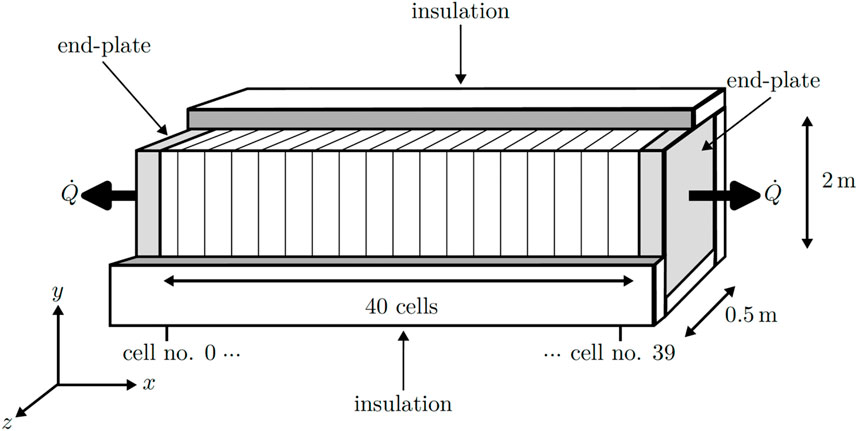
Figure 1. Schematic of the simulated industrial-sized stack with 1 m² cell-area.

The ECs are sandwiched between two endplates at the stack’s beginning and end. These endplates are not insulated toward the environment, leading to the assumption of free convection occurring at the lateral faces of the endplates. The model’s validation utilized temperature distributions provided by Krenz et al. (2023) on a stack level and the temperature distribution within a single cell as predicted by Bock et al. (2020b). Subsequently, the thermal conductivities obtained from the experimental setup were employed to simulate the temperature distribution within the stack.

2.2.1.1 Mesh

The mesh structure utilized in the model is illustrated in Supplementary Figure S2 for a single EC along with the two endplates. The mesh configuration of the single cell was then replicated for each EC within the stack (N^cell = 40 times) in the x-direction between the two endplates.

In the x-direction, each mesh cell corresponds to a distinct EC layer. However, the bipolar plates were subdivided into multiple layers, consisting of two FFs and one section of solid bipolar plate in between. Each segment has a thickness equivalent to one-third of the total bipolar plates thickness. The two FFs were further segmented into three layers; the actual FF and one boundary layer (BL) of δ^BL = 50 µm on each side, accounting for the convective heat-transfer resistance between the fluid in the FF and the surrounding solids. The dimensions of the boundary layer depend on the specific flow conditions inside the FF, but for simplicity, a constant value was approximated in this study. In the y-direction, each layer of the EC was discretized into N_mesh-cells,y = 21 cells of the mesh to analyse the temperature variation along the channels of the FF.

A boundary frame was subsequently incorporated around the mesh to enforce boundary conditions. Insulated boundaries were assumed on all sides, and these were implemented as Neumann boundary conditions, specifying the first derivative of temperature at the boundary cells to be zero. The only exception was observed at the FF inlets, where the temperature in the boundary cell was set to match the incoming fluid’s temperature using Dirichlet boundary conditions. The heat flux to the ambient in the endplates was introduced as a source term.

Temperature calculations were performed at the boundaries of each mesh cell, precisely at the interface between two EC layers. Consideration was given to energy exchange in the form of heat fluxes and mass flows between the mesh cells, with additional incorporation of heat sources and sinks attributable to the electrolysis reactions within the mesh cells.

2.2.1.2 Mass balance

The simplified mass flows within an individual EC in the simulation are illustrated in Supplementary Figure S2 alongside the mesh. In the case of parallel flow, the fluid inlet occurs at the initial mesh cell in the y-direction on both the anode and cathode sides of the bipolar plate. On the anode side, water (${\dot{m}}_{H_{2}O}^{in,a}$) and some oxygen (${\dot{m}}_{O_2}^{in,a}$) flow into the FF of the EC. On the cathode side, some water (${\dot{m}}_{H_{2}O}^{in,c}$) and hydrogen (${\dot{m}}_{H_2}^{in,}$) flow into the FF. For subsequent mesh cells in the y-direction, the products of the electrolysis reaction in the row below were added to the mass flow in the FF, while the reactants were subtracted. The oxygen mass flow in the mesh cell at y = j in an anodic FF ($\left.{\dot{m}}_{y=j}^{a,O_2}\right)$ was therefore calculated using Equation 3.

${\dot{m}}_{y=j}^{a,O_2}={\dot{m}}_{y=j-1}^{a,O_2}+{\dot{m}}_{y=j-1}^{R,O_2}(3)$

with the mass flow rate of oxygen (${\dot{m}}_{y=j-1}^{R,O_2}$) produced in the row of mesh cells below. This calculation involved the utilization of the Faraday constant ($F$), the cell area ($A_{y=j-1}$) of the mesh cell at $y=j-1$ considering its dimensions in the y- and z-directions, the current density ($i$), and the molar mass of elementary oxygen ($M^{O_2}$) as defined in Equation 4.

${\dot{m}}_{y=j-1}^{R,O_2}=\frac{i\cdot A_{y=j-1}}{4F}\cdot M^{O_2}(4)$

The mass flow of hydrogen on the cathode side (${\dot{m}}_{y=j}^{c,H_2}$) was calculated analogously with Equation 5.

${\dot{m}}_{y=j}^{c,H_2}={\dot{m}}_{y=j-1}^{c,H_2}+\frac{i\cdot A_{y=j-1}}{2F}\cdot M^{H_2}(5)$

The mass flow of water in the anodic FF (${\dot{m}}_{y=j}^{a,H_{2}O}$) undergoes a reduction owing to two distinct effects. Firstly, water serves as a reactant in the electrolysis reaction ($\left.{\dot{m}}_{y=j-1}^{R,H_{2}O}\right)$; and secondly, water is conveyed by the hydrogen ions through the electrolysis membrane to the cathode side (${\dot{m}}_{y=j-1}^{drag,H_{2}O}$) as described in Equation 6.

${\dot{m}}_{y=j}^{a,H_{2}O}={\dot{m}}_{y=j-1}^{a,H_{2}O}-{\dot{m}}_{y=j-1}^{R,H_{2}O}-{\dot{m}}_{y=j-1}^{drag,H_{2}O}(6)$

The mass flow of water consumed during the electrolysis reaction (${\dot{m}}_{y=j-1}^{R,H_{2}O}$) can be described analogously to the mass flow of hydrogen and oxygen with Equation 7.

${\dot{m}}_{y=j-1}^{R,H_{2}O}=\frac{i\cdot A_{y=j-1}}{2F}\cdot M^{H_{2}O}(7)$

The modeling of water drag (${\dot{m}}_{y=j-1}^{drag,H_{2}O}$) followed the methodology proposed by Springer et al. (1991), wherein they hypothesized an average of 2.5 water molecules being dragged across the membrane for each hydrogen ion in a fully humidified membrane. This relationship was assumed to exhibit a linear decrease with the level of humidification, as defined by Equation 8.

${\dot{m}}_{y=j-1}^{drag,H_{2}O}=2.5\cdot \frac{\lambda }{22}\cdot \frac{i\cdot A_{y=j-1}}{2F}\cdot M^{H_{2}O}(8)$

The mass flow of water on the cathode side (${\dot{m}}_{y=j}^{c,H_{2}O}$) correspondingly rises by the quantity of water transported through the membrane, and this can be expressed using Equation 9.

${\dot{m}}_{y=j}^{c,H_{2}O}={\dot{m}}_{y=j-1}^{c,H_{2}O}+{\dot{m}}_{y=j-1}^{drag,H_{2}O}(9)$

In the case of counter-flow operation, the previously mentioned equations remain applicable to the anodic FF, while the cathodic FF undergoes an inversion in the y-direction. Consequently, the inlet is situated at the last mesh-cell in the negative y-direction, and the fluid flows accordingly. The electrolysis reaction in the mesh-cells at $y=j+1$ was therefore considered when determining the mass flow in the mesh-cell $y=j$ in the cathode FF.

Within the PTLs, CLs, the membrane, and the flow field boundary layers (FF-BLs) facing the PTL, a mass flow in the x-direction was considered. It was presumed that precisely the amount of water utilized in the electrolysis reaction and transported through the membrane at $y=j$ flows in the positive x-direction through the anode side FF-BL, the PTL, and the ACL. Simultaneously, only the dragged water flows through the membrane, CCL, cathode side PTL, and FF-BL. The oxygen generated in the electrolysis reaction at $y=j$ was considered to flow in the negative x-direction through the anode CL, the anode-side PTL and FF-BL at $y=j$, while the hydrogen flows in the positive x-direction through the membrane, CCL, cathode-side PTL, and FF-BL.

The mass flow of water was further subdivided into gaseous and liquid forms in each mesh-cell to accommodate evaporation and condensation heat. To calculate the quantity of gaseous water in the fluid mixture, an ideal mixture of ideal gases was assumed for the gaseous phase. The mass flow of water in the gas phase under saturation conditions was determined using Equation 10 for the cathode side ($\left.{\dot{m}}_{sat.}^c\right)$ and Equation 11 for the anode side (${\dot{m}}_{sat.}^a$) (Krenz et al., 2023). These equations were derived from the ideal gas law.

${\dot{m}}_{sat.}^c=\frac{M^{H_{2}O}}{M^{H_2}}\cdot \frac{p_{sat.}^{H_{2}O}}{p-p_{sat.}^{H_{2}O}}\cdot {\dot{m}}^{H_2}(10)$

${\dot{m}}_{sat.}^a=\frac{M^{H_{2}O}}{M^{O_2}}\cdot \frac{p_{sat.}^{H_{2}O}}{p-p_{sat.}^{H_{2}O}}\cdot {\dot{m}}^{O_2}(11)$

The saturation pressure of water ($p_{sat.}^{H_{2}O}$) was computed was computed using the Antoine equation with coefficients from Roizard (Roizard, 2016).

The effective flow of gaseous water was determined by selecting the smaller value between ${\dot{m}}_{sat.}$ and the total mass flow of water within the corresponding mesh-cell. The remaining portion of the total mass flow of water in the cell was presumed to exist in the form of liquid water.

2.2.1.3 Cell potential

The cell potential is composed of the reversible cell voltage ($V_{rev}^{cell}$), and the activation (${\eta }_{act}$), ohmic (${\eta }_{ohm}$), and mass transfer (${\eta }_{mt}$) overpotentials. These potentials were individually computed for each electrolyzer cell and each row in the y-direction. The reversible cell voltage is contingent on the temperature and activity of the species involved in the reaction and can be determined using the Nernst equation. Assuming the presence of liquid water without gas bubbles in the CL, the Nernst equation can be expressed as Equation 12 (Krenz et al., 2023; Trinke, 2021).

$V_{rev}^{cell}=V_{rev}^{cell,\theta }+\frac{{RT}^{cell}}{2F}\mathit{ln}\left[{\left(\frac{c_{sat}^{c,H_2}}{c_{sat}^{c,H_2,\theta }}\right)}^1{\left(\frac{c_{sat}^{a,O_2}}{c_{sat}^{a,O_2,\theta }}\right)}^{\frac{1}{2}}{\left(a^{a,H_{2}O}\right)}^{-1}\right](12)$

The reversible cell potential under standard conditions ($V_{rev}^{cell,\theta }$) was determined through the calculation of Gibbs free energies at standard conditions. Here, R represents the universal gas constant, and F denotes the Faraday constant. The temperature pertinent to the reaction was taken as the mean temperature across the ACL, CCL, and membrane ($T^{cell}$). The activity of water ($a^{a,H_{2}O}$) was assumed to be unity for liquid water. The concentrations of oxygen at the ACL ($c_{sat}^{a,O_2}$) and hydrogen at the CCL ($c_{sat}^{c,H_2}$) were the saturation concentrations of the respective gases in water at a given temperature and pressure. $c_{sat}^{a,O_2,\theta }$ and $c_{sat}^{c,H_2,\theta }$ denote the concentrations of oxygen at the ACL and hydrogen at the CCL, respectively, under standard conditions (Krenz et al., 2023).

The saturation concentrations ($c_{sat}$) were computed utilizing the pressure ($p$) and Henry’s coefficient ($H_S$) according to Equation 13 (Krenz et al., 2023). The stack operation was assumed without pressurization, and ambient pressure (1 Atm) was considered uniform across the stack. Specifically, the temperature in the ACL was employed for determining the saturation concentration of oxygen, while the temperature in the CCL was utilized for assessing the saturation concentration of hydrogen under non-standard conditions.

$c_{sat}=p{H}_S\left(T\right)(13)$

Henry’s coefficient was calculated using the approach published by Ito et al. (2011).

The activation overpotential delineates losses attributable to electrochemical reaction activation, contingent upon the reaction rate. The correlation between the activation overpotential and the reaction rate, articulated in terms of current density, is presented by the Butler-Volmer equation. To compute the anodic activation overpotential, Krenz et al. provided a simplified approximation (Krenz et al., 2023). For the sake of comparability, the identical methodology was employed in this context.

Krenz et al. omits consideration of the cathodic activation overpotential (${\eta }_{act}^c$), deeming it negligible in comparison to the anodic activation overpotential (Krenz et al., 2023). Nevertheless, this overpotential could potentially impact the temperature distribution within individual ECs; therefore, it was incorporated into the present simulation. Given the absence of parameter values in existing literature for calculating the cathodic overpotential, a marginally distinct definition was adopted for this purpose (Equation 14 (Falcão and Pinto, 2020)).

${\eta }_{act}^c=\frac{{RT}^c}{{\alpha }_{ct}^{c}F}\mathit{arcsinh}\left(\frac{i}{2i_0^c}\right)(14)$

Here, the cathodic exchange current density is denoted as $i_0^c$. The temperature dependence of the cathodic charge transfer coefficient (${\alpha }_{ct}^c$) is frequently overlooked in the literature, attributed to its limited influence. Consequently, it has been omitted from consideration in this study as well. The temperature dependence of the cathodic exchange current density was determined analogously to the anodic exchange current density, employing Equation 15 (Correa et al., 2022).

$i_0^c=i_0^{c,ref}\mathit{exp}\left[\frac{E_{cd}^c}{R}\left(\frac{1}{298.15K}-\frac{1}{T^c}\right)\right](15)$

Here, $E_{cd}^c$ represents the activation energy (in J/mol K) associated with the cathodic exchange current density, $i_0^{c,ref}$ denotes the reference cathodic exchange current density at 298.15 K, and $T^c$ is the cathode temperature. The parameter values provided by Correa et al. (2022) were utilized to compute the cathodic activation overpotential, as experimental data for fitting the overpotential to the simulated system’s actual values was unavailable.

The ohmic overpotential (${\eta }^{ohm}$) encapsulates resistances opposing proton and electron fluxes. However, considering that electron flux resistances are markedly smaller than ionic resistances, they are often disregarded in the literature (Falcão and Pinto, 2020). In this context, the two primary resistances, comprising the ionic membrane resistance ($R_{el}^{mem}$) and the ionic contact resistance ($R_{el}^c$), were considered to calculate the ohmic overpotential, as outlined in Equation 16 (Krenz et al., 2023).

${\eta }^{ohm}=i\left(R_{el}^{mem}+R_{el}^c\right)(16)$

The contact resistance was presumed to remain constant across varying temperatures. The calculation of the ionic membrane resistance ($R_{el}^{mem}$) involved the utilization of the membrane’s ionic conductivity (${\sigma }^{mem}$) and thickness (${\delta }^{mem}$), as described by Equation 17.

$R_{el}^{mem}=\frac{{\delta }^{mem}}{{\sigma }^{mem}}(17)$

The ionic conductivity of the membrane is contingent upon its level of humidification denoted by the ratio of water molecules to sulfonic groups ($\lambda$) and the temperature ($T^{mem}$). Since $\lambda$ is usually a constant value when immersed in liquid water, the temperature is the main variable affecting proton conductivity in water electrolysers. This relationship can be approximated using the method outlined by Springer et al. (Springer et al., 1991), as expressed in Equation 18.

${\sigma }^{mem}=\left({\mathrm{{\rm K}}}^{mem}\lambda -0.326\right)\mathit{exp}\left[E^{mem}\left(\frac{1}{303K}-\frac{1}{T^{mem}}\right)\right](18)$

Where ${\mathrm{{\rm K}}}^{mem}$ is a linear fitting factor and $E^{mem}$ the activation energy.

The influence of mass transfer overpotentials becomes pronounced in cell voltage at elevated current densities, particularly when the reaction sites experience an overpopulation of reaction products, leading to a decline in reactant concentrations. In this study, calculations for the anode side mass transfer overpotentials (${\eta }_{mt}^a$) were conducted using Equation 19, and for the cathode side mass transfer overpotentials (${\eta }_{mt}^c$) using Equation 20 (Krenz et al., 2023).

${\eta }_{mt}^a=\frac{{RT}^a}{4F}\mathit{ln}\left(\frac{c_{supersat}^{a,O_2}}{c_{sat}^{a,O_2}}\right)(19)$

${\eta }_{mt}^c=\frac{{RT}^c}{2F}\mathit{ln}\left(\frac{c_{supersat}^{c,H_2}}{c_{sat}^{c,H_2}}\right)(20)$

The saturated concentrations were determined in a manner analogous to the process employed for the reversible cell potential, utilizing Henry’s law as described in Equation 14. Supersaturated concentrations denote the excess concentration of product gases within the CL, arising due to mass-transfer resistances. To compute concentrations in this supersaturated state ($c_{supersat}$), the production rate was determined based on the current density. The mass flow from the CL was considered directed towards the FF of the same electrode. Notably, the crossover of H₂ and O₂ through the membrane was disregarded in this context. The calculation of supersaturated concentrations was thus accomplished using Equation 21 (Trinke et al., 2017).

$c_{supersat}=\frac{\frac{i}{zF}+k_l{c}_{sat}}{k_l}(21)$

Here, $z$ denotes the number of electrons transferred per molecule, specifically 4 for O₂ and 2 for H₂. The mass transfer coefficient ($k_l$) is a parameter encompassing various mass transport resistances, including desorption, diffusion, and the processes of bubble formation, growth, and detachment associated with mass transport through the CL and PTL to the FF (Trinke et al., 2017).

2.2.1.4 Energy balance

Upon obtaining the overpotentials, which serve as heat sources within the EC, an energy balance is formulated to ascertain heat fluxes and temperature gradients within the ECs. Heat sinks and sources were allocated to the pertinent layers within the ECs, with calculations conducted individually for each row in the y-direction based on the prevailing conditions in the corresponding EC section. In addition to the heat contributions from the overpotentials, various heat sinks manifest within the EC. A portion of the heat is absorbed by the endothermic electrolysis reaction. The remaining heat is transferred to the fluids traversing the cell or is dissipated from the stack through the non-insulated endplates.

The heat generated by a specific overpotential (${\dot{Q}}_{overpot.}$) was computed by considering the current passing through the relevant EC section ($i$), incorporating the current density, the area of the mesh-cell in the y- and z-direction ($A$), and the overpotential ($\eta$) calculated for the respective section Equation 22.

${\dot{Q}}_{overpot.}=iA\eta (22)$

The heat flux resulting from the anodic activation and mass-transfer overpotentials was assigned to the ACL, while the heat generated by the cathodic activation and mass-transfer overpotentials was directed to the CCL. The heat associated with ohmic overpotentials was allocated to the electrolyte membrane.

The molar reversible heat required for the electrolysis reaction ($Q_{m,rev.}$) is calculated from the difference between reaction Enthalpy and reaction Gibbs Energy that is provided directly by electrical energy. The reversible molar heat was subsequently multiplied by the reaction rate within the corresponding mesh-cell to obtain the reversible heat flow (${\dot{Q}}_{rev.}$) using Equation 23.

${\dot{Q}}_{rev.}=Q_{m,rev.}\cdot \frac{iA}{2F}(23)$

The heat flow was then distributed as a sink, with half allocated to the ACL and the remaining half to the CCL, following the approach suggested by Bock et al. (Bock et al., 2020b). The electrolysis reaction is divided into two half-cell reactions, one occurring at the anode and the other at the cathode. It is assumed that the entropy change of the water electrolysis reaction is equally divided between the anode and the cathode. This assumption is supported by empirical half-cell entropy measurements conducted by Fang et al. (Fang et al., 2008). The heat transfer coefficient (h_t) was taken as 45 W m⁻² K⁻¹, as recommended by Krenz et al. (Krenz et al., 2023). Subsequently, the heat flux was calculated based on the temperature difference between the outer side of the endplates and ambient temperature (T^amb. = 294.15 K). The heat flow was then determined, considering the area of the respective mesh-cell, and using sizes in y- and z-direction. This calculated heat flow was incorporated into the simulation as a heat sink applied to the endplates.

Utilizing the mass flows within the ECs in both x- and y-directions, along with the corresponding temperatures, an enthalpy balance was established for each mesh-cell. This involved summing up the enthalpies of incoming and outgoing mass flows to address heat transported by the mass flow. An ideal mixture assumption was made for all fluids, and the total change in enthalpy was determined by setting up an energy balance for each component $\alpha$ in the fluid Equation 24. Due to the principle of energy conservation, the total change in enthalpy equates to the amount of heat exchanged with the fluids. This heat flow ($\dot{Q}$) was implemented as a source/sink in the respective mesh-cell.

$\dot{Q}={\displaystyle \sum _{\alpha ,out}}{H}_{out}^{\alpha }\cdot {\dot{m}}_{out}^{\alpha }-{\displaystyle \sum _{\alpha ,in}}{H}_{in}^{\alpha }\cdot {\dot{m}}_{in}^{\alpha }(24)$

The specific enthalpies ($H_{in/out}^{\alpha }$) of the component $\alpha$ were computed based on the enthalpy $H_0^{\alpha }$ at the reference temperature ($T_0$ = 343.15 K), assuming ideal gases and incompressible fluids. In the case of gases, the specific isobaric heat capacity (c_p) was applied Equation 25, while for liquids, the specific isochoric heat capacity (c_v) was considered Equation 26.

$H_{in/out}^{\alpha }=H_0^{\alpha }+c_p^{\alpha }\cdot \left(T_{in/out}-T_0\right)(25)$

$H_{in/out}^{\alpha }=H_0^{\alpha }+c_v^{\alpha }\cdot \left(T_{in/out}-T_0\right)(26)$

The enthalpies at reference temperatures and the specific heat capacities at $T_0$ were computed utilizing the Cantera library in Python. It was simplistically assumed that the fluids share the same temperature as the solids in the respective mesh-cell. The typical heat transfer coefficients between water and steel were used to estimate an effective thermal conductivity of the BL. The thermal conductivities in this range were then fitted to the thermal gradients previously published by Bock et al. (Bock et al., 2020b). To assess and compare the efficiency of the electrolysis reaction in various simulation scenarios, the voltage efficiency according to the higher heating value (${ϵ}_V^{HHV}$) is employed. It is calculated using the cell voltage ($V^{cell}$) and the thermo-neutral voltage ($V_{thn.}$) as shown in Equation 27 (Krenz et al., 2023). The efficiency is computed separately for each row in the y-direction in every EC within the stack. The arithmetic mean of all calculated values is then considered as the stack’s voltage efficiency.

${ϵ}_V^{HHV}=\frac{V_{thn.}}{V^{cell}}(27)$

Upon incorporating all sources and sinks into the mesh, the resultant heat fluxes between the mesh-cells and, consequently, the temperature gradients could be determined.

2.2.1.5 Heat transfer

To depict the temperature distribution resulting from conduction with sources and sinks, the Fourier-Biot equation was established by formulating a three-dimensional energy balance rooted in Fourier’s law (Lienhard IV, 2006). Assuming a uniform temperature in the z-direction, the correlation can be expressed as Equation 28 to characterize a two-dimensional temperature distribution in the x- and y-directions.

$c\rho \cdot \frac{\partial T}{\partial t}={\kappa }_x\frac{{\partial }^{2}T}{\partial x^2}+{\kappa }_y\frac{{\partial }^{2}T}{\partial y^2}+\dot{q}(28)$

where $t$ is time, ${\kappa }_{x/y}$ represents thermal conductivity in the x and y directions, $\dot{q}$ denotes the heat flux source term (W/m³), $c$ signifies the specific heat capacity, and $\rho$ signifies the density (kg/m³).

In this study, the thermal conductivities measured for the membrane and CLs were utilized in both x- and y-directions, assuming isotropic thermal conductivities, as commonly assumed in literature (Bhaiya et al., 2014; Bock et al., 2020b; Burheim, O. S., 2017). The ACLs and CCLs were assumed to have identical thermal conductivities due to their similar composition (Zhang et al., 2022). While the thermal conductivity in carbon-fibre-based fuel cell PTL is highly anisotropic, with in-plane conductivity ten times higher than through-plane conductivity, sintered EC PTL is postulated to have isotropic properties (Bock et al., 2020b). Considering the fibrous structure of the titanium felt PTL, an anisotropic behaviour like carbon fibre was assumed, using the measured through-plane conductivity ${\kappa }_x$ and assuming the in-plane thermal conductivity ${\kappa }_y$ to be ten times ${\kappa }_x$, as reported by Bock et al. (Bock et al., 2020b). Wet thermal conductivities at 16 bar compaction pressure were employed for all layers of the simulated PEMEC to emulate conditions within the actual EC, despite PEMECs typically operating at compaction pressures of 20–30 bar (Borgardt et al., 2019). This was due to the limitation of the thermal conductivity measurement rig used in this study, which had a maximum compaction pressure of 16 bar. Negligible contact resistances were assumed between individual layers.

Thermal conductivities for the isotropic stainless steel bipolar plates were obtained from literature. In the FFs, thermal conductivity was presumed to be half the value of pure stainless steel, with the assumption that half the cell area consists of ribs made of stainless steel and the other half comprises channels with negligible across-the-channel conductivity. This geometry was not based on any specific design commercially available, but assumed a conventional serpentine design with 50% ribs and 50% channels. Thermal conductivity in the BLs of the FFs was determined by fitting using literature values for temperature gradients between fluid in the FF and adjacent solids in EC FFs (Bock et al., 2020b).

2.2.1.6 Solver

To adapt the Fourier-Biot equation to the mesh and solve it using the Euler method, discretization was performed employing second-order finite differences in space and first-order forward differences in time Equation 29. Given the unknown heat capacity for most EC layers, the time-step was coupled with the thermal diffusivity of the Fourier-Biot equation, resulting in the equivalent time-step ($∆t_e$). Since the focus lies on the steady-state temperature, any resulting distortion in the time dimension is deemed irrelevant.

$T_{i,j}^{n+1}=T_{i,j}^n+∆t_e\left[\frac{{\kappa }_{x,i,j}\frac{T_{i+1,j}-T_{i,j}}{x_{i+1,j}-x_{i,j}}+{\kappa }_{\mathrm{{\rm X}},i-1,j}\frac{T_{i-1,j}-T_{i,j}}{x_{i,j}-x_{i-1,j}}}{x_{i+1,j}-x_{i,j}}+\frac{{\kappa }_{y,i,j}\frac{T_{i,j+1}-T_{i,j}}{y_{i,j+1}-y_{i,j}}+{\kappa }_{y,i,j-1}\frac{T_{i,j-1}-T_{i,j}}{y_{i,j}-y_{i,j-1}}}{y_{i,j+1}-y_{i,j}}+\dot{q}\right](29)$

In the nth iteration, denoted as $n$, the positions in the x-direction and y-direction are represented by i and j, respectively. The volumetric-specific heat flux, denoted as $\dot{q}$, is employed to impart the computed heat sources and sinks onto the temperature field. The stability of this scheme is assured under the condition stipulated in Equation 30 (Moin, 2010).

$∆t_e\le \frac{1}{4\left[\mathit{max}\left(\frac{{\kappa }_x}{∆x^2}\right)+\mathit{max}\left(\frac{{\kappa }_y}{∆y^2}\right)\right]}(30)$

Equation 29 was systematically addressed through iterative solutions until the convergence criteria, $\left|T^{n+1}-T^n\right|<{ϵ}_T$, where ${ϵ}_T$ represents the maximum allowable temperature change per iteration, was satisfied.

The cell voltage, typically supplied by power electronics and characterized by uniformity across each cell owing to the high electrical conductivity of the bipolar plates (Krenz et al., 2023), serves as a critical parameter. To determine current densities ($i$) within each mesh cell under specific conditions, the current density underwent iteration concurrently with temperature, utilizing the ratio between the voltage derived from reversible cell voltage and overpotentials ($V^{cell,n}$) and the voltage set-point ($V_{set}^{cell}$), as defined in Equation 31.

$i^{n+1}=i^n\frac{V_{set}^{cell}}{V^{cell,n}}(31)$

To guarantee satisfactory convergence of the current density, an additional convergence criterion was incorporated ensuring that the absolute difference between the current at iteration $\left|i^{n+1}-i^n\right|<{ϵ}_i$. Unique values for ${ϵ}_i$ and ${ϵ}_T$ were selected for each simulation scenario to secure convergence.

2.2.1.7 Parameters

The calculations in this work utilized most parameters from the investigation conducted by Krenz et al. (Krenz et al., 2023) to maintain comparability with existing literature. For cell-level considerations not covered by Krenz et al. (Krenz et al., 2023), certain parameters were adopted from other studies. A comprehensive summary of all parameters can be found in Table 2.

Table 2

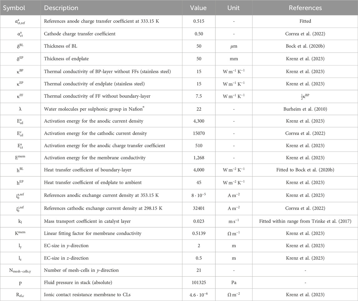
Table 2. Simulation parameters not varied between simulation cases.

2.2.2 Model analysis

To analyse the accuracy of the simulation results depicting the conditions within a PEMEC stack, various measures were implemented. Firstly, the convergence of the simulation was confirmed for each simulation cycle; and secondly, a comprehensive analysis procedure was applied to ensure the fidelity of the simulation implementation. These tests included a mesh refinement study, examination of simulations with varying thermal conductivity values, and a comparison of simulated temperature distribution with relevant literature.

To guarantee the convergence of the simulation, stringent convergence criteria (${ϵ}_i$ and ${ϵ}_T$) were set, ensuring that temperatures and current densities in the mesh remained relatively stable during the final 10% of iterations with maximum allowed deviations of 0.05 K for temperatures or 0.001 A cm⁻² for current density. Additionally, an energy balance check was conducted, ensuring that the total difference between heat produced and consumed in one EC was below 0.1% of the maximal heat produced in a single mesh cell.

As part of the model implementation analysis, a mesh refinement study was executed by doubling the number of mesh cells in the y-direction to $N_{mesh-cells,y}=42$ for a counter-flow stack to eliminate potential mesh-related influences on simulation results. The x-direction mesh cell count remained unchanged, as the temperature gradient within individual cell layers was assumed to be linear. Counter-flow configuration was chosen for its more complex temperature distribution over the ECs, necessitating a finer resolution. Furthermore, to verify the model’s correctness, simulations were conducted for parallel flow with both high (15 W m⁻¹ K⁻¹) and low (2 W m⁻¹ K⁻¹) thermal conductivity values in all layers (except for FFs and BLs). The conductivity in the Flow Fields was consistently set at half the conductivity of the bipolar plates, and the thermal conductivity in the BLs remained constant as listed in Table 2.

Lastly, the assumptions made during modelling were cross-analysed against existing literature. Due to limited available data on temperature distribution within ECs, simulated temperatures were compared to predictions from validated models at both the cell and stack levels. For the single PEMEC, the model was compared to Bock et al.'s (Bock et al., 2020b) work, replicating their conditions by utilizing their thermal conductivities, fluid temperature, and layer thicknesses. The model was validated on an EC-level by comparing cross-sections through all layers in the middle of the EC to Bock et al.'s results for different PTLs with varying thermal conductivities. Similarly, for an industrial-sized EC stack, the model was compared to Krenz et al.'s (Krenz et al., 2023) simulation results for both parallel and counter-flow configurations. The parameters used to reproduce the results from Bock et al. (Bock et al., 2020b) and Krenz et al. (Krenz et al., 2023) are summarized in Supplementary Table S1.

2.2.3 Simulated scenarios

Following the model analysis, an examination of the influence of various parameters on the temperature distribution across the PEMEC stack was undertaken. To achieve this, five distinct scenarios were defined. The initial simulation aimed to predict the temperature distribution within the stack, replicating the conditions described by Krenz et al. (Krenz et al., 2023). The thermal conductivities considered for this base scenario corresponded to the upper boundary of uncertainty observed in this study (i.e., the maximum measured conductivities). This involved the variation of individual parameters for both parallel flow (scenario 1) and counter-flow (scenario 2) configurations while maintaining the current density at 2.0 A cm⁻². All specific parameter values employed in each scenario are detailed in Supplementary Table S2.

The third scenario compared the titanium felt PTL used in other scenarios with a sintered titanium PTL in a counter-flow configuration. Mean values of the thermal conductivities of wet-sintered PTL, as measured by Bock et al. (Bock et al., 2020b), were employed for both the anodic and cathodic PTL. Uniform thermal conductivity values were applied for both in-plane and through-plane conductivities, aligning with the isotropic behavior postulated by Bock et al. for the sintered PTL (Bock et al., 2020b).

The fourth scenario explored the impact of higher current densities on the maximal temperatures in counter-flow configurations by increasing the current density to 3 A cm⁻² (i.e., high current density). In the fifth scenario, a temperature variation was introduced by increasing the temperature by 3 K at the inlet of the cathodic FF and decreasing it by 3 K at the inlet of the anodic FF using the counter-flow configuration. This investigation aimed to assess the impact on the temperature gradient within the MEA and explore potential efficiency benefits.

3 Results

3.1 Measured thermal conductivity and compressibility

The thermal conductivity and compressibility of the material layers employed in the PEMEC were determined through ex-situ measurements using the heat-flux method. The following section presents the measurements conducted for the materials utilized in the PEMEC.

The thermal conductivities of the EC membrane, CL, and MEA are detailed in Table 3 for single humidification measurements.

Table 3

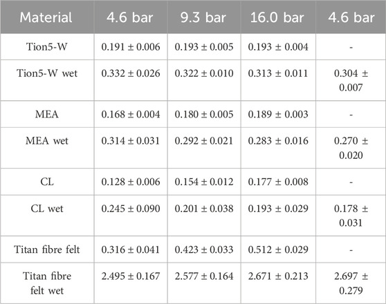
Table 3. Measured thermal conductivities of EC materials in W m⁻¹ K⁻¹ at different compaction pressures.

All wet thermal conductivity measurements displayed significant hysteresis effects between the first and second measurements at 4.6 bar, attributed to drying as samples had been pre-compressed during dry measurements. To ascertain whether drying was due to compression or time-dependent, measurements were repeated with re-humidification between each pressure step. The measured compressions of the samples are presented in Supplementary Table S3.

Supplementary Table S4 compares the humidification levels of these measurements with those described earlier. Deviations between measurements with and without re-humidification were within measurement uncertainties for both humidification level and thermal conductivities. Consequently, thermal conductivities measured with re-humidification are not separately discussed here.

3.2 Simulated temperature distribution

Upon assessing the thermal conductivities across distinct layers within the EC, a computational model was employed to predict the temperature distribution within a PEMEC stack. Subsequently, an exposition of the model analysis results. Following this, the simulated temperature distribution within the stack is elucidated under varied operational parameters.

3.2.1 Model analysis

The initial presentation pertains to the outcomes of comprehensive tests, including a mesh refinement study and an exploration of variations in thermal conductivities. Subsequently, the model is subjected to analysis with pertinent literature, initially at the individual cell level and subsequently at the aggregate stack level.

Doubling the number of cells in the y-direction yielded inconsequential impacts on simulation outcomes, as evidenced in Figure 2 for the central cell within the stack (EC no. 21). It is established that employing 21 mesh cells in the z-direction is adequately representative for modelling the pertinent temperature gradients in this study.

Figure 2

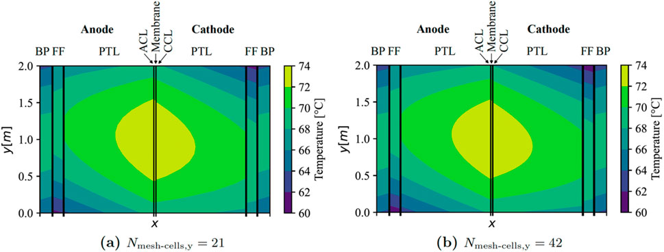
Figure 2. Results of the mesh refinement study for middle cell in stack with counter-flow (x-axis not to scale). BP, bipolar plate; FF, flow field; PTL, porous transport layer; ACL, anode catalyst layer; and, CCL, cathode catalyst layer.

The initial phase of analysis involved the simulation of temperature distribution within an individual EC. The outcomes obtained through the model developed in this study, employing parameters derived from Bock et al. (Bock et al., 2020b), are illustrated in Figure 3A. The simulation utilized the V-i characteristic outlined by Bock et al. (Bock et al., 2020b) at a current density of 3 A cm⁻². Discrepancies were observed in the temperatures at the outer side of the FFs, with the results exhibiting a 2 K reduction compared to Bock et al. (Bock et al., 2020b). Conversely, a consistent increase in temperature within the FFs, including their BLs, was observed in both works. Notably, both simulations indicated a markedly higher temperature in the ACL compared to the CCL, with the highest temperature occurring at the ACL-membrane interface.

Figure 3

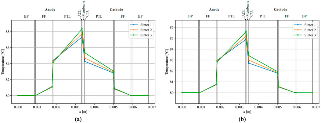
Figure 3. Simulated temperatures within a single EC with i = 3 A cm⁻² (A), and simulated temperature-gradients using parameters from Bock et al. (2020b) and overpotentials from Krenz et al. (2023) (B).

Temperature gradients over the anodic PTL and ACL exhibited similarities, registering approximately 4 K for the least conductive material (Sinter 3 with 5.6 W m⁻¹ K⁻¹), 3.5 K for Sinter 2 (6.9 W m⁻¹ K⁻¹), and approximately 2.8 K for the most conductive PTL (Sinter 1 with 8.2 W m⁻¹ K⁻¹). On the cathodic side, temperature gradients aligned only for the highly conductive PTLs, with a slight discrepancy observed for Sinter 3 in the present model. Furthermore, maximal temperatures were marginally lower in this study’s model, reaching 87.4°C with Sinter 1°C and 88.5°C with Sinter 3, as opposed to Bock et al.'s measured values of 89.1°C with Sinter 1°C and 92.0°C with Sinter 3 (Bock et al., 2020b). Notably, on the anodic side of the FF BL, the PTL with the highest conductivity exhibited a higher temperature than PTLs with lower conductivities, diverging from the observations in Bock et al.'s results (Bock et al., 2020b).

Bock et al. (Bock et al., 2020b) assumed elevated overpotentials, leading to a more pronounced voltage-current characteristic compared to the findings by Krenz et al. (Krenz et al., 2023). Subsequently, the model underwent a secondary iteration at a current density of i = 3 A cm⁻², employing the overpotentials delineated by Krenz et al. (Krenz et al., 2023). While the temperature distribution exhibited consistency in its configuration, the temperatures registered a decrease overall, with a peak temperature of approximately 85.7°C observed on the anode side of the membrane when utilizing a Sinter 3 PTL, and approximately 85 °C with Sinter 1 (Figure 3B).

Furthermore, the analysis of the simulation was conducted for a PEMEC stack, operating at an average current density of 2 A cm⁻², utilizing parameters sourced from the study by Krenz et al. (Krenz et al., 2023). The simulated temperature distribution across a stack in parallel flow is illustrated in Figure 4. Projections indicated temperatures at the FF inlets ranging from 60 °C within the FFs to 65 °C in the membranes. Conversely, at the outlet side, temperatures peaked at approximately 67 °C in the FFs and 71 °C in the membranes. Notably, the outer cells of the stack exhibited slightly lower temperatures, with a reduction of 1.4 K on the left side and 1.1 K on the right side compared to the maximal temperature in the middle cells. This observation aligns closely with the anticipated mean temperature distribution in the ECs as predicted by Krenz et al. (Krenz et al., 2023).

Figure 4

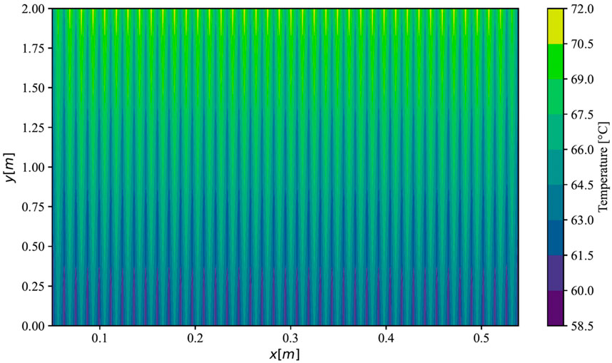
Figure 4. Simulated temperatures within a 40 cell EC stack at i = 2 A cm⁻² in parallel flow.

The simulated heat flux in the x-direction within a cross-section through the middle of ECs in the stack (y = 1 m) is depicted in Figure 5, aiming to contrast the heat flux entering the anodic fluid with the predictions proposed by Krenz et al. (Krenz et al., 2023). Positive values denote a heat flux directed towards the cathode side, while negative values indicate a flux towards the anode side. The heat flux at the inner (right) BL of the anodic FF, represented by the point to the left of the most negative heat flux within each EC, was approximately −4,200 Wm⁻² in the middle of the stack. Furthermore, the heat flux at the interface with the outer (left) BL of the anodic FF was projected to be close to zero for all ECs except the first. The value of the heat flux at the inner BL of the anodic FF therefore signifies the heat flux entering the anodic fluid. In the initial EC on the left, a notable heat flux was observed, departing from the anodic FF towards the BP on the left, resulting in a lower heat flux absorbed by the anodic fluid at approximately 3,200 Wm⁻². Similarly, the heat flux into the anodic fluid in the last cell of the stack (on the right side) was lower than in the middle of the stack. These observations align well with the conclusions drawn by Krenz et al. (Krenz et al., 2023).

Figure 5

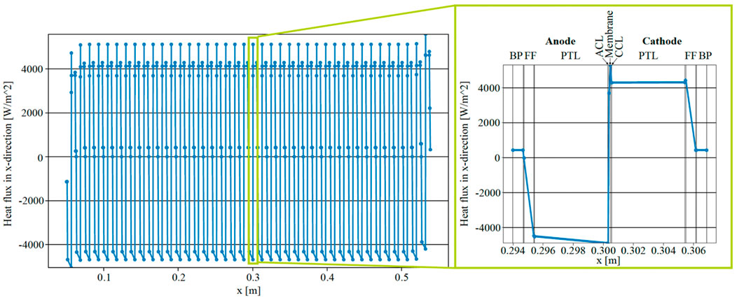
Figure 5. Simulated heat flux within a 40 cell EC stack at y = 1 m and i = 2 A cm⁻² with parallel flow.

As the final step in the analysis process, the simulated temperatures were juxtaposed with the outcomes reported by Krenz et al. (Krenz et al., 2023) for an EC stack operating in a counter-flow configuration at a mean current density of 2 A cm⁻². The simulated maximal temperatures were observed near the center of the cells at y = 1 m, registering approximately 73.5°C in the membranes and around 69 °C in the FFs (Figure 6). Notably, these temperatures exceeded the maximal temperatures observed in parallel flow. In the outer ECs, the temperature exhibited a somewhat greater impact, with a reduction in maximal temperature of 3.4 K on the left side and 2.6 K on the right side compared to parallel flow. These findings align with the conclusions drawn by Krenz et al. (Krenz et al., 2023). In general, the predicted conditions demonstrate a substantial agreement with the existing literature.

Figure 6

Figure 6. Simulated temperatures within a 40 cell EC stack at i = 2 A cm⁻² with counter-flow.

3.2.2 Simulated scenarios

A summary of voltage efficiencies under both parallel and counter-flow conditions is provided in Supplementary Table S5, while Supplementary Table S6 compiles the maximal temperature gradients observed within an individual cell in the stack. Further elaboration on the intricate temperature distributions within the stack and cells is presented in subsequent sections.

3.2.2.1 Scenario 1: Maximal measured conductivities for parallel flow

Utilizing thermal conductivities at the upper boundary of uncertainty based on values obtained in this study for PEMEC components resulted in a maximum temperature gradient of 16.0 K within a single cell under parallel flow conditions. The temperature distribution within the central cell of the stack is illustrated in Figure 7A. The highest temperature was recorded between the ACL and the membrane, adjacent to the outlets of the FFs, reaching 76.0°C. Although the temperature in the anodic half-cell consistently exceeded that in the cathodic half-cell, the distribution was otherwise comparable. Throughout the stack, a uniform temperature distribution was projected for all middle cells (Figure 7B). However, the first and last cells adjoining the endplates exhibited noticeably lower temperatures, with a maximum of 74.0°C in the initial cell and 75.1°C in the terminal cell.

Figure 7

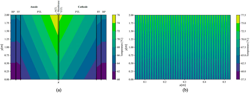
Figure 7. Simulated temperature distribution in middle cell (A); (x-axis not to scale) and the whole stack (B) under parallel flow using maximal values of measured conductivities.

3.2.2.2 Scenario 2: Maximal measured conductivities for counter-flow

Given consistent thermal conductivities under counter-flow conditions, the maximal temperature gradient within the ECs increased by 1.1 K–17.1 K (Figure 8). The maximal temperature was observed between the ACL and the membrane, slightly above the centre of the cell along the y-direction, registering at 77.1°C. In the cathodic half-cell, the maximal temperatures were attained slightly below the middle of the cell; therefore, in closer proximity to the outlet of the respective half-cell.

Figure 8

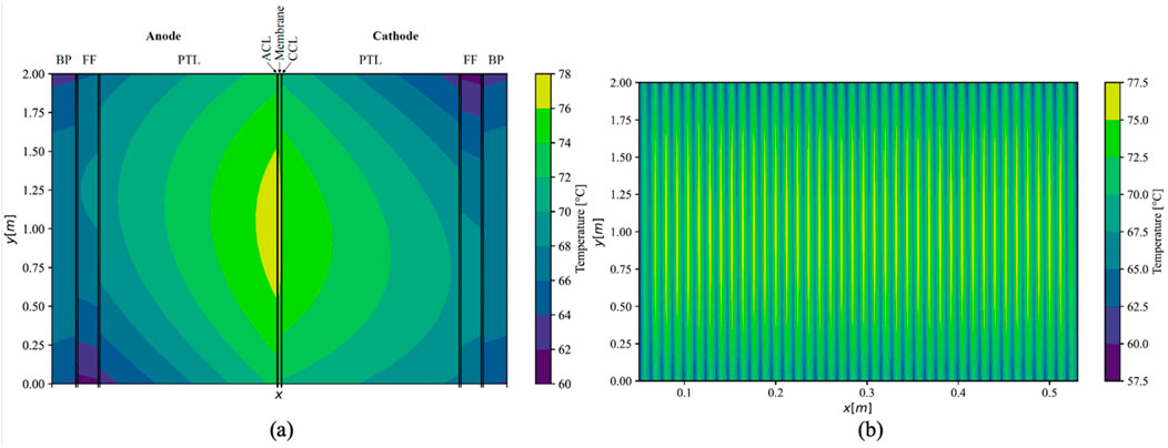
Figure 8. Simulated temperature distribution in middle cell (A); (x-axis not to scale) and the whole stack (B) under counter-flow using maximal values of measured conductivities.

In contrast to parallel flow, the current density exhibited a more even distribution across the cell in the y-direction, featuring a lower maximal value and a higher minimal value, while maintaining a consistent mean current density of 2 A cm⁻² in both scenarios. Additionally, under counter-flow conditions, a slightly elevated voltage efficiency was achieved, reaching 75.2%, as opposed to 75.0% observed under parallel flow. Due to the augmented efficiency in the counter-flow arrangement, this flow configuration was deemed more pertinent and is expanded upon in greater detail in the subsequent scenarios.

The temperature distribution was notably consistent among all cells situated in the middle of the stack, with discernible lower temperatures in the outer cells. As depicted in Supplementary Figure S3a, the temperature distribution within the initial cell on the left side of the stack exhibited a more uniform spread between the anodic and cathodic sides within the MEA compared to the middle cells. However, an increase in thermal gradient was observed in the anodic half-cell. The maximal temperature in this cell was recorded at 73.4°C, approximately 4 K lower than that observed in the middle cells of the stack. Conversely, in the terminal cell on the right side of the stack, a higher temperature gradient between the anodic and cathodic sides of the MEA was noted (Supplementary Figure S3b). Here, the temperature decrease was more pronounced in the cathodic half-cell. The maximum cell temperature in this instance was approximately 75.0°C, positioning it between the temperature observed in the initial cell and that in the middle of the stack.

3.2.2.3 Scenario 3: Sinter PTL

An additional simulation was conducted employing the maximum measured conductivity values for the membrane and CLs, while utilizing literature values for the sintered titanium PTL. The simulated temperature distribution within the central cell of the stack is portrayed in Figure 9A, specifically for the counter-flow configuration. The maximal temperature in the cell was recorded at 73.6°C, indicating a reduction of approximately 3.5 K compared to the base scenario, accompanied by a maximal thermal gradient of 13.6 K within a single cell. Furthermore, the voltage efficiency experienced a marginal decline of 0.2%, in comparison to the base scenario. Notably, the temperature gradient witnessed a decrease, particularly in the x-direction, and to a lesser extent in the y-direction due to the isotropic conductivity in sinter PTL and non-isotropic in felt PTL. This resulted in an alteration of the thermal gradient’s shape compared to the base scenario. Although the temperature distribution across the stack maintained similarity to the base scenario, it shifted towards lower temperatures, exhibiting a slightly heightened cooling effect on the outer cells situated on the right side.

Figure 9

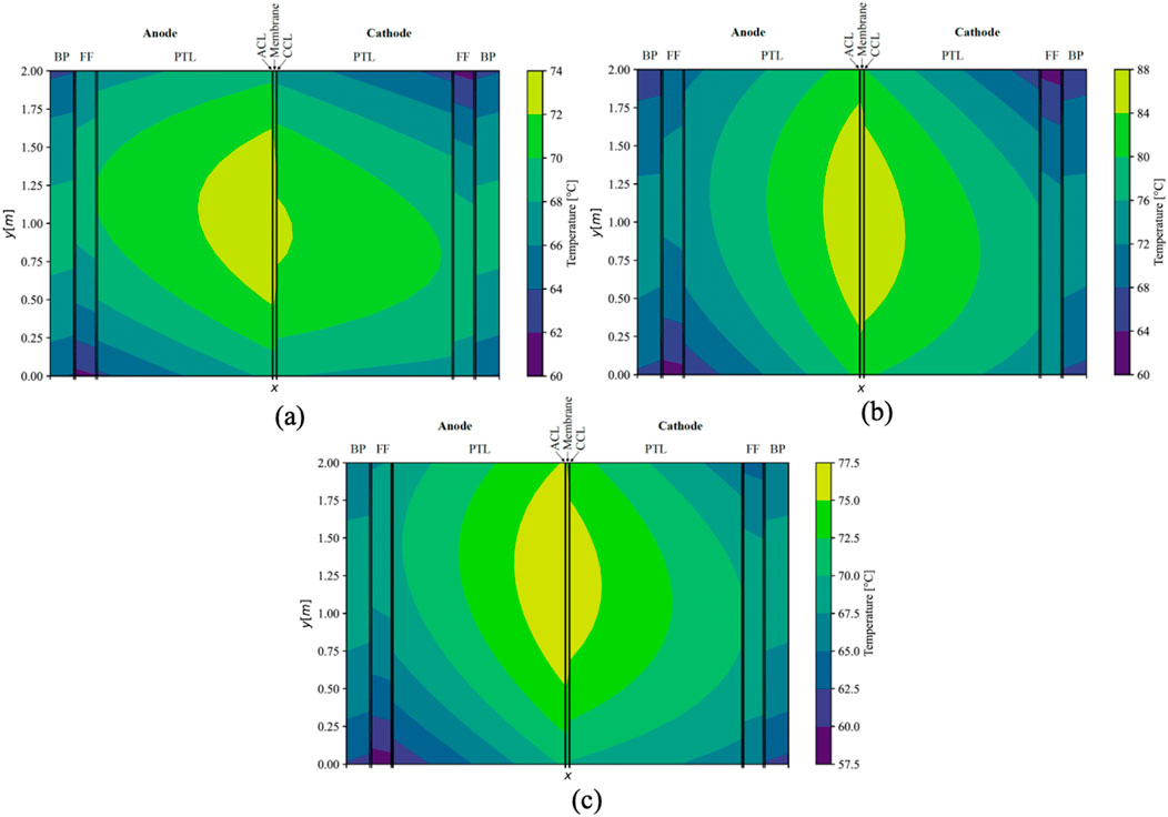
Figure 9. Simulated temperature distribution in middle cell (x-axis not to scale) under counter-flow using sintered PTLs (A), with a mean current density of 3 A cm⁻² (B), and with a warmer inlet-temperature in the cathodic FF (C).

3.2.2.4 Scenario 4: High current density

Upon increasing the current density to 3 A cm⁻², a deviation from the base scenario was observed, resulting in a 9 K elevation in the maximal temperature under counter-flow conditions, reaching 87.0°C. This escalation consequently led to an amplified temperature gradient within the ECs in the stack, surpassing one-half to reach 27.0 K. Concurrently, the voltage efficiency experienced a notable decline, decreasing by 3.6%. The temperature distribution within the ECs remained relatively unchanged for the central cell in the counter-flow stack (Figure 9B). The thermal gradient between the FFs and the adjacent MEA increased from approximately 10 K at 2 A cm⁻² to 14 K in the middle of the ECs (y = 1 m). Moreover, under a constant mass flow of water, the temperature within the FFs exhibited a significant increase of 5 K in this cross-section.

3.2.2.5 Scenario 5: Warmer cathode

After modifying the conditions, the temperature at the inlet of the cathodic FF was increased to 63 °C, while concurrently decreasing the anodic inlet temperature to 57 °C. This adjustment resulted in an overall temperature increase in the cathodic half-cell and a corresponding decrease in the anodic half-cell. The thermal gradients within the ECs experienced a rise of 3.4 K, while maintaining an almost constant maximal temperature of 77.4°C under counter-flow conditions. Notably, altering the inlet temperatures did not significantly alleviate the thermal gradient across the MEA (Figure 9C). Consequently, the voltage efficiency remained unchanged. In this cross-section, the temperature in the FFs deviated by only 0.8 K in the cathodic FF and 0.3 K in the anodic FF from the scenario with uniform temperatures at the FF inlets.

4 Conclusion

In the initial phase of the study, thermal conductivities, and compressibility’s of PEMEC Tion5-W PFSA membrane, CL, and platinized titanium felt PTL were systematically assessed under varying pressures and humidification levels. Subsequently, a 2D simulation of the temperature distribution within an industrial-scale PEMEC stack with a 1 m² cell area was conducted. This simulation considered thermal gradients within individual cells by incorporating the experimentally measured thermal conductivities.

The through-plane thermal conductivities were measured ex-situ using the heat flux method and were validated against established materials such as PEEK, demonstrating good agreement with existing literature. The EC CL, comprising iridium ruthenium oxide anodic and platinum black cathodic CLs, exhibited a similar order of magnitude in thermal conductivity as the Tion5-W PFSA membrane but with significantly higher compressibility. For the platinized titanium felt PTL, the dry thermal conductivities were approximately double those of the membrane or CL, yet below literature values for other titanium based PTLs. An increase of about five times in conductivity was observed when humidified and over 50% under pressure, with no notable compressibility.

The 2D simulation underwent comparison analysis on both cell and stack levels using established models from literature. The simulated conditions within the stack, considering parallel and counter-flow configurations based on measured thermal conductivities, predicted temperature gradients within cells under specific flow and current density conditions. Notably, the counter-flow arrangement demonstrated a 0.2% increase in voltage efficiency, with maximal temperatures occurring between the ACL and membrane in the middle of the ECs in counter-flow and at the FF outlets in parallel flow. However, such marginal improvements from computational studies cannot confirm that counter-flow has better voltage efficiency. Therefore, further empirical studies are required to assess whether there is an advantage in terms of voltage efficiency when using parallel or counter-flow configurations.

Replacing the measured through-plane thermal conductivity values of titanium felt PTL with the higher literature values for sintered PTL resulted in lower thermal gradients. Membrane and CL thermal conductivities had a comparatively lower impact. Therefore, it is crucial to consider the through-plane thermal conductivity of PTL during the design process to minimize thermal gradients and maximize current densities within the stack. The in-plane thermal conductivity of the PTL exhibited lower relevance due to the extended FFs in industrial-sized electrolysers.

Increasing the current density to 3 A cm⁻² heightened thermal gradients in both parallel and counter-flow configurations, leading to a 3.6% reduction in voltage efficiency. The advantage of the counter-flow arrangement in terms of voltage efficiency slightly increased with higher current density, with the maximal temperature remaining lower in parallel flow.

To explore potential efficiency benefits through lower thermal gradients over the MEA, the inlet temperature of the fluid was manipulated at the cathode and anode sides. However, due to the high thermal conductivity of the BPs, fluid temperatures between two adjacent anodic and cathodic FFs annealed quickly inside the ECs, with no discernible impact on performance or maximal temperatures in the cells.

In the design process of future electrolysers, particularly at high current densities, careful consideration of the temperature distribution within single ECs on a stack level is imperative to prevent membrane overheating or necessitate increased safety margins due to unknown temperature gradients. The through-plane thermal conductivity and thickness of PTLs have been identified as critical factors to limit thermal gradients, underscoring the importance of their consideration during material selection for future electrolysers. In future research endeavors, the thermal conductivity of diverse PTL materials should be investigated to identify high-conductive options capable of reducing thermal gradients in next-generation PEM electrolyzers. Additionally, remeasuring the thermal conductivity of titanium felt PTL with custom-made samples of varying thickness can help eliminate potential contact resistance effects, as well as measuring the in-plane thermal conductivity. Refining the developed model by incorporating separate temperatures for fluids and solids, using advanced heat transfer models within the porous layers, can also enhance the accuracy of calculating the cooling effect of mass flows through the MEA. Furthermore, optimization of the model is still required to find the ideal flow rates, flow field thicknesses and boundary layer thicknesses.

The primary objective of this study was to measure the thermal conductivities of PEMEC components and then establish a modeling framework for simulating PEMEC stacks at the resolution of the individual cell level. Owing to the scarcity of empirical investigations in this domain, there are limited studies regarding temperature fluctuations in PEMECs available. Consequently, the present model lacks validation against a physical PEMEC apparatus as there is still a barrier to empirical measurements in PEMECs (as with their fuel cell alternative) due to compaction pressure and size. Thus, the proposed modeling framework provided must undergo validation via physical experimentation in forthcoming research endeavors as relevant parameters become available.

Data availability statement

The original contributions presented in the study are included in the article/Supplementary Material, further inquiries can be directed to the corresponding author.

Author contributions

BE: Data curation, Formal Analysis, Investigation, Methodology, Software, Validation, Visualization, Writing–original draft, Writing–review and editing. MA: Project administration, Resources, Supervision, Writing–original draft, Writing–review and editing. OB: Conceptualization, Methodology, Project administration, Resources, Writing–original draft, Writing–review and editing. JL: Conceptualization, Investigation, Methodology, Project administration, Resources, Supervision, Writing–original draft, Writing–review and editing.

Funding

The author(s) declare that no financial support was received for the research, authorship, and/or publication of this article.

Acknowledgments

The authors acknowledge the support from the ENERSENSE research initiative.

Conflict of interest

The authors declare that the research was conducted in the absence of any commercial or financial relationships that could be construed as a potential conflict of interest.

The author(s) declared that they were an editorial board member of Frontiers, at the time of submission. This had no impact on the peer review process and the final decision.

Publisher’s note

All claims expressed in this article are solely those of the authors and do not necessarily represent those of their affiliated organizations, or those of the publisher, the editors and the reviewers. Any product that may be evaluated in this article, or claim that may be made by its manufacturer, is not guaranteed or endorsed by the publisher.

Supplementary material

The Supplementary Material for this article can be found online at: https://www.frontiersin.org/articles/10.3389/fceng.2024.1384772/full#supplementary-material

References

Ahadi, M., Andisheh-Tadbir, M., Tam, M., and Bahrami, M. (2016). An improved transient plane source method for measuring thermal conductivity of thin films: deconvoluting thermal contact resistance. Int. J. Heat. Mass Transf. 96, 371–380. doi:10.1016/j.ijheatmasstransfer.2016.01.037

CrossRef Full Text | Google Scholar

Ahadi, M., Tam, M., Saha, M. S., Stumper, J., and Bahrami, M. (2017). Thermal conductivity of catalyst layer of polymer electrolyte membrane fuel cells: Part 1–Experimental study. J. Power Sources 354, 207–214. doi:10.1016/j.jpowsour.2017.02.016

CrossRef Full Text | Google Scholar

Asmatulu, R., Khan, A., Adigoppula, V. K., and Hwang, G. (2018). Enhanced transport properties of graphene-based, thin Nafion® membrane for polymer electrolyte membrane fuel cells. Int. J. Energy Res. 42, 508–519. doi:10.1002/er.3834

CrossRef Full Text | Google Scholar

Bhaiya, M., Putz, A., and Secanell, M. (2014). Analysis of non-isothermal effects on polymer electrolyte fuel cell electrode assemblies. Electrochimica Acta 147, 294–309. doi:10.1016/j.electacta.2014.09.051

CrossRef Full Text | Google Scholar

Bock, R., Hamre, B., Onsrud, M. A., Karoliussen, H., Seland, F., and Burheim, O. S. (2019). The influence of argon, air and hydrogen gas on thermal conductivity of gas diffusion layers and temperature gradients in PEMFCs. ECS Trans. 92, 223–245. doi:10.1149/09208.0223ecst

CrossRef Full Text | Google Scholar

Bock, R., Karoliussen, H., Pollet, B. G., Secanell, M., Seland, F., Stanier, D., et al. (2020a). The influence of graphitization on the thermal conductivity of catalyst layers and temperature gradients in proton exchange membrane fuel cells. Int. J. Hydrog. Energy 45, 1335–1342. doi:10.1016/j.ijhydene.2018.10.221

CrossRef Full Text | Google Scholar

Bock, R., Karoliussen, H., Seland, F., Pollet, B. G., Thomassen, M. S., Holdcroft, S., et al. (2020b). Measuring the thermal conductivity of membrane and porous transport layer in proton and anion exchange membrane water electrolyzers for temperature distribution modeling. Int. J. Hydrog. Energy 45, 1236–1254. doi:10.1016/j.ijhydene.2019.01.013

CrossRef Full Text | Google Scholar

Bock, R., Shum, A., Khoza, T., Seland, F., Hussain, N., Zenyuk, I. V., et al. (2016). Experimental study of thermal conductivity and compression measurements of the gdl-mpl interfacial composite region. ECS Trans. 75, 189–199. doi:10.1149/07514.0189ecst

CrossRef Full Text | Google Scholar

Bock, R., Shum, A. D., Xiao, X., Karoliussen, H., Seland, F., Zenyuk, I. V., et al. (2018). Thermal conductivity and compaction of GDL-MPL interfacial composite material. J. Electrochem. Soc. 165, F514–F525. doi:10.1149/2.0751807jes

CrossRef Full Text | Google Scholar

Borgardt, E., Giesenberg, L., Reska, M., Müller, M., Wippermann, K., Langemann, M., et al. (2019). Impact of clamping pressure and stress relaxation on the performance of different polymer electrolyte membrane water electrolysis cell designs. Int. J. Hydrog. Energy 44, 23556–23567. doi:10.1016/j.ijhydene.2019.07.075

CrossRef Full Text | Google Scholar

Burheim, O., Vie, P. J. S., Pharoah, J. G., and Kjelstrup, S. (2010). Ex situ measurements of through-plane thermal conductivities in a polymer electrolyte fuel cell. J. Power Sources 195, 249–256. doi:10.1016/j.jpowsour.2009.06.077

CrossRef Full Text | Google Scholar

Burheim, O. S. (2017). (Invited) review: PEMFC materials' thermal conductivity and influence on internal temperature profiles. ECS Trans. 80, 509–525. doi:10.1149/08008.0509ecst

CrossRef Full Text | Google Scholar

Burheim, O. S., Crymble, G. A., Bock, R., Hussain, N., Pasupathi, S., du Plessis, A., et al. (2015). Thermal conductivity in the three layered regions of micro porous layer coated porous transport layers for the PEM fuel cell. Int. J. Hydrog. Energy 40, 16775–16785. doi:10.1016/j.ijhydene.2015.07.169

CrossRef Full Text | Google Scholar

Burheim, O. S., Ellila, G., Fairweather, J. D., Labouriau, A., Kjelstrup, S., and Pharoah, J. G. (2013). Ageing and thermal conductivity of porous transport layers used for PEM fuel cells. J. Power Sources 221, 356–365. doi:10.1016/j.jpowsour.2012.08.027

CrossRef Full Text | Google Scholar

Burheim, O. S., and Pharoah, J. G. (2017). A review of the curious case of heat transport in polymer electrolyte fuel cells and the need for more characterisation. Curr. Opin. Electrochem. 5, 36–42. doi:10.1016/j.coelec.2017.09.020

CrossRef Full Text | Google Scholar

Burheim, O. S., Pharoah, J. G., Lampert, H., Vie, P. J., and Kjelstrup, S. (2011). Through-plane thermal conductivity of PEMFC porous transport layers. J. Fuel Cell. Sci. Technol. 8. doi:10.1115/1.4002403

CrossRef Full Text | Google Scholar

Burheim, O. S., Su, H., Hauge, H. H., Pasupathi, S., and Pollet, B. G. (2014). Study of thermal conductivity of PEM fuel cell catalyst layers. Int. J. Hydrog. Energy 39, 9397–9408. doi:10.1016/j.ijhydene.2014.03.206

CrossRef Full Text | Google Scholar

Chen, T., Liu, S., Zhang, J., and Tang, M. (2019). Study on the characteristics of GDL with different PTFE content and its effect on the performance of PEMFC. Int. J. Heat. Mass Transf. 128, 1168–1174. doi:10.1016/j.ijheatmasstransfer.2018.09.097

CrossRef Full Text | Google Scholar

Correa, G., Marocco, P., Muñoz, P., Falagüerra, T., Ferrero, D., and Santarelli, M. (2022). Pressurized PEM water electrolysis: dynamic modelling focusing on the cathode side. Int. J. Hydrog. Energy 47, 4315–4327. doi:10.1016/j.ijhydene.2021.11.097

CrossRef Full Text | Google Scholar

Falcão, D. S., and Pinto, A. (2020). A review on PEM electrolyzer modelling: guidelines for beginners. J. Clean. Prod. 261, 121184. doi:10.1016/j.jclepro.2020.121184

CrossRef Full Text | Google Scholar

Fang, Z., Wang, S., Zhang, Z., and Qiu, G. (2008). The electrochemical Peltier heat of the standard hydrogen electrode reaction. Thermochim. Acta 473, 40–44. doi:10.1016/j.tca.2008.04.002

CrossRef Full Text | Google Scholar

Ito, H., Maeda, T., Nakano, A., and Takenaka, H. (2011). Properties of Nafion membranes under PEM water electrolysis conditions. Int. J. Hydrog. Energy 36, 10527–10540. doi:10.1016/j.ijhydene.2011.05.127

CrossRef Full Text | Google Scholar

Kavadias, K. A., Apostolou, D., and Kaldellis, J. K. (2018). Modelling and optimisation of a hydrogen-based energy storage system in an autonomous electrical network. Appl. Energy 227, 574–586. doi:10.1016/j.apenergy.2017.08.050

CrossRef Full Text | Google Scholar

Khandelwal, M., and Mench, M. M. (2006). Direct measurement of through-plane thermal conductivity and contact resistance in fuel cell materials. J. Power Sources 161, 1106–1115. doi:10.1016/j.jpowsour.2006.06.092

CrossRef Full Text | Google Scholar

Krenz, T., Weiland, O., Trinke, P., Helmers, L., Eckert, C., Bensmann, B., et al. (2023). Temperature and performance inhomogeneities in PEM electrolysis stacks with industrial scale cells. J. Electrochem. Soc. 170, 044508. doi:10.1149/1945-7111/accb68

CrossRef Full Text | Google Scholar

Kumar, S. S., and Lim, H. (2022). An overview of water electrolysis technologies for green hydrogen production. Energy Rep. 8, 13793–13813. doi:10.1016/j.egyr.2022.10.127

CrossRef Full Text | Google Scholar

Lienhard IV, J. H. (2006). A heat transfer textbook. MA, United States: Cambridge.

Google Scholar

Moin, P. (2010). Fundamentals of engineering numerical analysis. Cambridge University Press.

Google Scholar

Nafchi, F. M., Afshari, E., and Baniasadi, E. (2022). Thermal and electrochemical analyses of a polymer electrolyte membrane electrolyzer. Int. J. Hydrog. Energy 47, 40172–40183. doi:10.1016/j.ijhydene.2022.05.069

CrossRef Full Text | Google Scholar

Roizard, D. (2016). in Antoine equation. Editors E. Drioli,, and L. Giorno (Berlin, Heidelberg: Encyclopedia of Membranes. Springer Berlin Heidelberg), 97–99. doi:10.1007/978-3-662-44324-8_26

CrossRef Full Text | Google Scholar

Schiebahn, S., Grube, T., Robinius, M., Tietze, V., Kumar, B., and Stolten, D. (2015). Power to gas: technological overview, systems analysis and economic assessment for a case study in Germany. Int. J. Hydrog. Energy 40, 4285–4294. doi:10.1016/j.ijhydene.2015.01.123

CrossRef Full Text | Google Scholar

Schuler, T., De Bruycker, R., Schmidt, T. J., and Büchi, F. N. (2019). Polymer Electrolyte Water Electrolysis: correlating porous transport layer structural properties and performance: Part I. Tomographic analysis of morphology and topology. J. Electrochem. Soc. 166, F270–F281. doi:10.1149/2.0561904jes

CrossRef Full Text | Google Scholar

Shum, A. D., Parkinson, D. Y., Xiao, X., Weber, A. Z., Burheim, O. S., and Zenyuk, I. V. (2017). Investigating phase-change-induced flow in gas diffusion layers in fuel cells with X-ray computed tomography. Electrochimica Acta 256, 279–290. doi:10.1016/j.electacta.2017.10.012

CrossRef Full Text | Google Scholar

Springer, T. E., Zawodzinski, T. A., and Gottesfeld, S. (1991). Polymer electrolyte fuel cell model. J. Electrochem. Soc. 138, 2334–2342. doi:10.1149/1.2085971

CrossRef Full Text | Google Scholar

Trinke, P., 2021. Experimental and model-based investigations on gas crossover in polymer electrolyte membrane water electrolyzers.

Google Scholar

Trinke, P., Bensmann, B., and Hanke-Rauschenbach, R. (2017). Current density effect on hydrogen permeation in PEM water electrolyzers. Int. J. Hydrog. Energy 42, 14355–14366. doi:10.1016/j.ijhydene.2017.03.231

CrossRef Full Text | Google Scholar

Van der Vegt, A. K., and Govaert, L. E., 2003. Polymeren: van keten tot kunststof. DUP Blue Print.

Google Scholar

Yasutake, M., Noda, Z., Tachikawa, Y., Lyth, S. M., Matsuda, J., Nishihara, M., et al. (2022). Temperature distribution analysis of PEM electrolyzer in high current density operation by numerical simulation. ECS Trans. 109, 437–450. doi:10.1149/10909.0437ecst

CrossRef Full Text | Google Scholar

Yuan, X.-Z., Shaigan, N., Song, C., Aujla, M., Neburchilov, V., Kwan, J. T. H., et al. (2022). The porous transport layer in proton exchange membrane water electrolysis: perspectives on a complex component. Sustain. Energy Fuels 6, 1824–1853. doi:10.1039/d2se00260d

CrossRef Full Text | Google Scholar

Zhang, K., Liang, X., Wang, L., Sun, K., Wang, Y., Xie, Z., et al. (2022). Status and perspectives of key materials for PEM electrolyzer. Nano Res. Energy 1, e9120032. doi:10.26599/nre.2022.9120032

CrossRef Full Text | Google Scholar

Zhao, J., Liu, H., and Li, X. (2023). Structure, property, and performance of catalyst layers in proton exchange membrane fuel cells. Electrochem. Energy Rev. 6, 13. doi:10.1007/s41918-022-00175-1

CrossRef Full Text | Google Scholar