 Jacob G. Wasserfall
 Corné J. Coetzee
- Department of Mechanical and Mechatronic Engineering, University of Stellenbosch, Stellenbosch, South Africa
A fully coupled computational fluid dynamics (CFD) and discrete element method (DEM) model was calibrated using a draw down test (DDT) under submerged conditions. Momentum smoothing and cell clustering were used to model particles that were larger than the cells. The DEM input parameter values were initially set equal to those calibrated for the dry conditions. Under submerged conditions, results showed that the particle-particle coefficient of friction and the drag modifier had an influence on the results. It was found that the drag modifier had to be calibrated, while the particle-particle coefficient of friction, calibrated under dry conditions, could be used for the submerged conditions. A vertical suction pipe validation experiment was conducted. The suction pipe had a constant diameter, but the fluid velocity and the distance the pipe opening was held from the granular bed were varied. The amount of mass (particles) removed as well as the size of the cavity that formed in the material bed were measured and compared to model predictions. The results showed that using the parameter values calibrated in the DDT, too much material was removed (error of 30%). Removing the drag modifier (setting it equal to unity) significantly improved the results (error of 6%). It is concluded that due to the difference in flow mechanism (particle-induced in the DDT versus fluid-induced in the suction pipe), the DDT is not a suitable experiment to calibrate the input parameter values for a suction pipe. It is proposed that the flow mechanism and dynamics of the granular material and the fluid in the calibration experiment should be similar to that of the final application being investigated.
1 Introduction
Fluid-particle systems play an integral part in natural and industrial processes. The behaviour of these two-phase systems poses a unique problem to both experimental analysis and numerical modelling due to the complex interactions that such systems can exhibit. Accurate numerical modelling of fluid-particle systems would give a better understanding of the fundamental interactions that govern the bulk behaviour of two-phase systems. This allows for a more comprehensive design approach for industrial processes that handle these materials, e.g., discharge hoppers (Hesse et al., 2020), pneumatic conveyors (Lavrinec et al., 2020), pumps (Gao et al., 2020), etc.
Such models can also be applied to applications such as riverbeds and soil surface erosion (Bravo-Blanco et al., 2017; Guo and Yu, 2017; Jaiswal et al., 2024). In this study, however, the main application is deep sea mining where mineral rich gravel is sucked from the ocean floor. And accurate model of this process will provide valuable insight and can be used as a design tool. However, such a model first need to be calibrated in a laboratory setup where repeatable tests can be performed. Here the draw down test is proposed as a calibration test due to its relative ease of operation and data measurement, and also its successful use in calibrating Discrete Element Models (DEM) of dry and cohesive materials.
1.1 Modelling techniques
Considered separately, both the fluid and particle phases have extensive fields dedicated to their numerical modelling and numerous options, both commercial and open source, for implementing these models. Computational Fluid Dynamics (CFD) is a commonly used continuum-based approach for modelling fluid systems while DEM provides an effective simulation technique for modelling the behaviour of granular materials, especially when the discrete interaction between particles needs to be resolved. Coupling these two methods allows two-phase systems to be modelled by having each method resolve one phase of the system and prescribing interactions between them.
1.2 DEM calibration
DEM models require input parameters that represent the properties of the real particles being modelled. Calibration describes the methods employed to determine these input parameters, and is typically placed into one of two approaches (Marigo and Stitt, 2015; Coetzee, 2017).
The bulk calibration approach (BCA) makes use of experiments that measure specific bulk material behaviours or properties (macro scale), such as the angle of repose (AOR) for example,. These experiments are replicated numerically, and model input parameters systematically changed until the experimental bulk behaviour is closely replicated. When this bulk calibration method is employed, the bulk behaviour (flow mechanism) of the material in the calibration experiment should be comparable to that of the intended application (Coetzee, 2017).
On the other hand, the direct measuring approach (DMA) makes use of measuring material properties at the particle or contact level (meso scale). These properties are then directly used as input parameter values in the model, such as the particle-wall coefficient of friction for example,. In some cases, these measurements are simple to conduct, while in others they can be very difficult, especially when particles are very small (particle-particle coefficient of friction for example,). This method does, however, not guarantee accurate predictions of the material’s bulk behaviour. Even if some properties could be accurately measured, the model still relies on assumptions and simplifications that should be accounted for. The modelled particle shape, for example, is almost always a simplification of the physical particles, and the contact models are only simplified representations of the real physics. To account for this, the BCA ensures that the input parameters are calibrated in such a way that the model accurately predicts the material bulk behaviour despite the assumptions and simplifications (Coetzee, 2017). The two approaches (BCA and DMA) are often used in combination, as was also the case in this study.
1.3 Draw down tests
When multiple input parameters are calibrated, at least the same number of independent bulk properties should be measured for a well-posed solution (Coetzee, 2017; Roessler et al., 2019). A unique set of values for two or three input parameters often can not be determined from only a single bulk property such as the angle of repose for example,. The draw down test (DDT) is a single experiment in which up to four bulk properties can be easily measured.
In the DDT, two containers (boxes) are placed one above the other. The upper box acts as a discharge bin and has a trapdoor at the bottom which can be quickly released to allow the material to flow into the lower box. This allows for the shear angle,
Calibration has been mostly restricted to single-phase DEM applications while fluid-particle simulations often implement material input parameters without calibration in a two-phase environment (Jing et al., 2019; Chen et al., 2021). Not much is known about the effects that fluid-particle interactions have on the effectiveness of purely DEM-calibrated input parameters. By constructing a DDT that is capable of both single-phase and two-phase calibration tests, numerical input parameters can be calibrated using DEM and CFD-DEM and their differences compared.
1.4 CFD-DEM coupling
CFD-DEM simulations are constrained by coupling limitations that restrict the size difference between the CFD fluid mesh and the DEM particle size, that is, specifically the use of large particles in small fluid meshes (Akhshik et al., 2016; Wang et al., 2019; Zhou et al., 2019). This limits the range of applications for CFD-DEM simulations, creating a gap in the understanding of fluid-particle interactions. Recent adaptations of CFD-DEM coupling software have shown promise in lessening these constraints, allowing applications previously unfeasible (Song and Park, 2020; Zhang et al., 2023; Zhou et al., 2024).
2 Numerical models
The software package, Simcenter STAR-CCM+ (Siemens Digital Industries Software, 2021), was used in this study. The numerical formulation for the particle phase, the fluid phase, the coupling, and the source smoothing is presented below.
2.1 Particle phase
The Discrete Element Method (DEM) is a numerical modelling technique used to simulate granular material by considering its discrete particles and the interactions between them. The displacement, velocity, orientation, and angular velocity of each particle are stored and used along with the forces and moments acting on the particle to solve equations of motion. These equations as well as all particle interactions are resolved during each timestep. Considering only the translation of a particle, the following general formulation (Eq. 1) of motion can be constructed,
where
where
2.2 Fluid phase
In contrast to DEM, conventional fluid mechanics does not consider individual particles but rather views fluids as a continuum. The fluid behaviour is governed by the continuity and Navier-Stokes equations,
where
where
2.3 Fluid-particle coupling
The total fluid-particle interaction force,
where
where
where
where
with
Where the particle sphericity
2.4 Source smoothing
To ensure model accuracy and stability, the fluid mesh is required to be at least 3 times the size of the largest particle diameter (Wang et al., 2019; Zhou et al., 2019; He et al., 2024). This criterion poses a problem when large particle diameters are encountered in small domains since a small mesh size is required to accurately resolve the fluid flow field and the mesh cannot accommodate both an upper and lower size constraint. To overcome this limitation, the so-called “source smoothing” method employed by the software Simcenter STAR-CCM+ (Siemens Digital Industries Software, 2021) was used. Using source smoothing, fluid cells are clustered together forming a coarser fluid mesh when resolving the fluid-particle interaction (Song and Park, 2020; Zhang et al., 2023; Zhou et al., 2024). Large particles that span multiple cells are assigned to these larger clusters for the purposes of determining momentum exchange and porosity calculations. The momentum and void fraction contributions of particles are then virtually spread between all the cells within the clusters. A representation of the effect of source smoothing is shown in Figure 1 where the cell cluster length has been set to twice that of the largest cell. As shown in Figure 1A, when source smoothing is not active, each particle is assigned to a single cell, determined by the position of its centroid, and interacts only with that cell until its centroid moves outside the boundaries of the cell. Within a cell cluster, a particle’s centroid only needs to be within the boundaries of a single cell to influence all the cells in the cluster, Figure 1B.
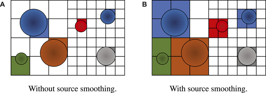
Figure 1. The presence of particles as seen from the perspective of the fluid mesh, where shaded cells indicate the particle-fluid interaction: a red particle for example, interacts with the red cells (A). Without source smoothing (B). With source smoothing.
3 Materials and methods
3.1 Particle size and shape
Figure 2A shows the experimental material divided into three distinct particle size distributions (PSDs) which were each individually tested. However, for conciseness, only the results from the 8–16 mm and 16–32 mm are presented here (the experimental results of 4–8 mm are given as Supplementary Material). The physical particles used in this study were far from spherical in shape, therefore it was opted to make use of the multi-sphere particle approach as shown in Figure 2B. For more details on multi-sphere particles, also called clumps or composite particles, see for example, Coetzee (2016) and Lu et al. (2022).
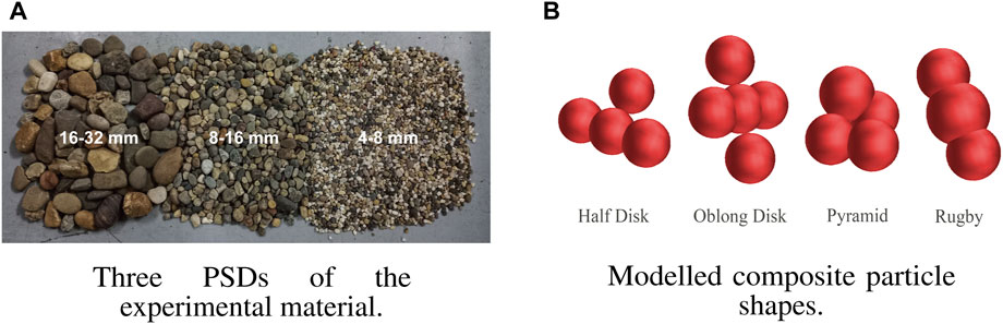
Figure 2. The experimental material and the modelled particle shapes (A). Three PSDs of the experimental material (B). Modelled composite particle shapes.
Among some researchers, it has become common practise to model non-spherical particles as spherical, and then to account for the shape by adding rolling resistance (Wensrich and Katterfeld, 2012; Wensrich et al., 2014; Roessler et al., 2019). On the other hand, some researchers have a firm believe that the combination of rolling resistance and spherical particles cannot account for all granular behaviour, and that the shape should be more accurately modelled using polyhedra (Govender, 2021; Feng, 2023; Govender et al., 2023), spherical harmonics (Radvilaitė et al., 2016), or surfaces of revolution (Yuan, 2024) for example,.
A study by Coetzee (2020) showed that the bulk behaviour of non-spherical particles can be accurately modelled using either spherical particles with rolling resistance, or non-spherical particles without rolling resistance. Similar to the current study, a draw down test was used for calibration. The advantage of using spherical particles with rolling resistance is that the computation time is reduced. However, it requires the calibration of an additional parameter, namely, the rolling friction. Since the effects of the coefficients of sliding and rolling friction are difficult to isolate, these two parameters need to be calibrated together and a unique combination must be found (Roessler et al., 2019; Coetzee, 2020). On the other hand, when modelling the particles as non-spherical, computation time increases, but the rolling friction is excluded as a parameter that needs calibration. The latter philosophy was used in the current study.
For modelling the drag force and buoyancy of the particles accurately, the maximum and minimum projected areas of the modelled particles (expressed as a function of their volume) were compared to that of a sample of the physical particles. The range of projected areas of the modelled particles matched well with that of the physical particles for both PSDs.
3.2 Material properties
Using direct measurement techniques, the particle density
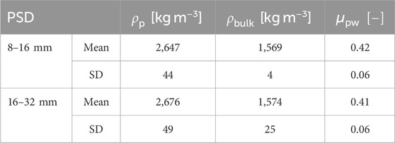
Table 1. Measured material properties.
3.3 Draw down test
3.3.1 Experiment
A large-scale DDT rig was constructed to accommodate the large particle sizes of the granular material to be calibrated. Figure 3A shows the constructed test rig on the left. The free-hanging upper tank, suspended inside the larger lower tank, was connected to two HBM (RSCC 200 kg) tension loadcells which would allow the change in mass in the upper tank to be measured and, therefore, the mass flow rate. A pneumatically operated gate attached to the lower tank could be activated to allow material to flow from the upper tank to the lower tank. A long vertical cylindrical drain was placed in the centre of the lower tank and allowed both water and granular material to be removed at the end of an experiment.
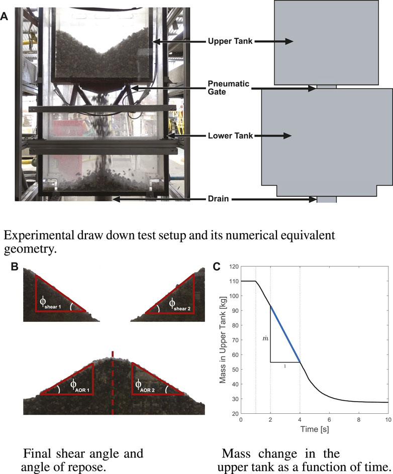
Figure 3. The experimental and DEM setup of the draw down test showing the final material configuration in a typical test under dry conditions and the mass in the upper tank (A). Experimental draw down test setup and its numerical equivalent geometry (B). Final shear angle and angle of repose (C). Mass change in the upper tank as a function of time.
To conduct the submerged DDTs, the test rig was filled with water until both the lower and upper tanks were submerged. Granular material could then be added to the upper tank. The submerged tests followed the same experimental procedure as in the dry tests, although the test rig needed to be filled and drained of water between each test.
3.3.2 Model
For single-phase (dry) conditions, the experimental DDT rig geometry was replicated numerically, as shown on the right in Figure 3A, which describe the boundaries of the DEM domain. Figure 3B shows the final state of the material at the end of the test, and Figure 3C shows the mass in the upper tank as a function of time. A Hertz-Mindlin contact model was used, which required a particle elastic modulus
The numerical DDT geometry was adjusted slightly to better accommodate the addition of the CFD fluid model. Figure 4 shows the model geometry, dimensions and fluid mesh, where parts of the mesh have been hidden for clarity. A trimmed cell mesher was employed which used square cells to mesh the model geometry. This produced a well-conditioned mesh as most of the geometry, except the cylindrical drain, aligned with the square mesh. To avoid the low-quality cells that would emerge due to the cylindrical shape of the drain, the drain was modelled as rectangular to align with the mesh but preserved its volume.
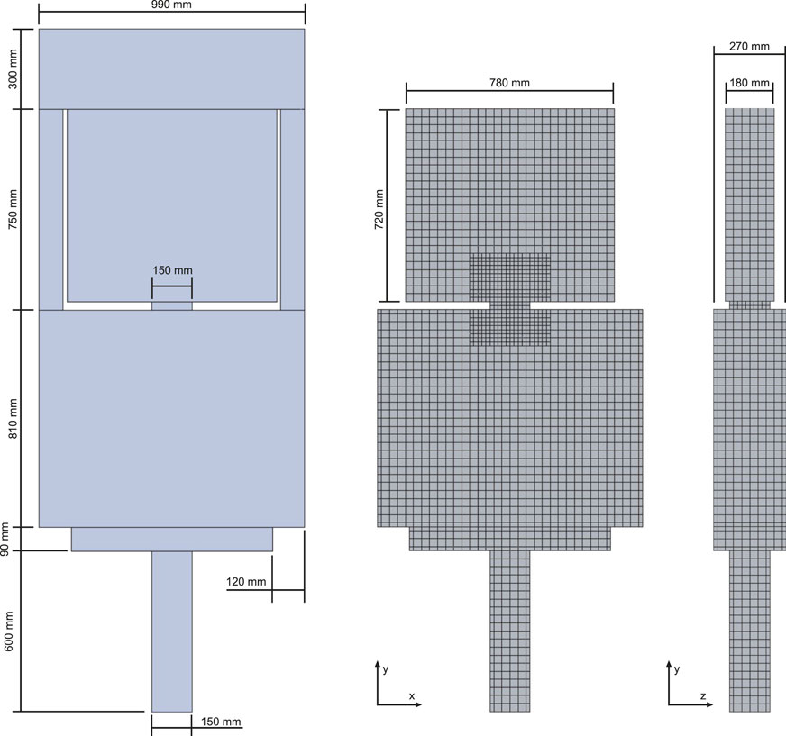
Figure 4. CFD-DEM model geometry and mesh of the draw down test.
A base mesh size of 30 mm was used which covered most of the model geometry without the need for refinement, as shown in Figure 4. The cells around the opening between the upper and lower tank were refined to 15 mm, half the base mesh size. The upper boundary of the model was made a constant pressure outlet while the rest of the geometry surfaces acted as wall boundaries. A second-order implicit unsteady solver was used to solve the fluid phase and a
3.4 Vertical suction pipe test
To verify the material calibration procedure, a vertical suction pipe experiment was devised which would be replicated numerically using the calibrated input parameters found for the two PSDs under submerged conditions.
3.4.1 Experiment
The experimental setup of the vertical pipe test is shown in Figure 5A where
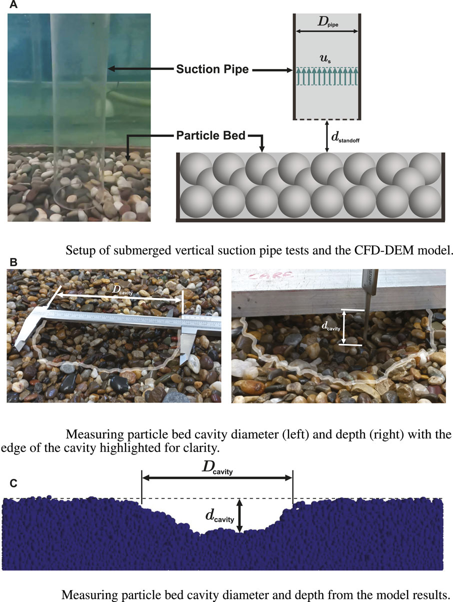
Figure 5. The (A) setup of the submerged suction pipe experiment and model and the measurement of the cavity properties in (B) the experiment and (C) the model (A). Setup of submerged vertical suction pipe tests and the CFD-DEM model (B). Measuring particle bed cavity diameter (left) and depth (right) with the edge of the cavity highlighted for clarity (C). Measuring particle bed cavity diameter and depth from the model results.
A series of tests were conducted for both PSDs and different fluid velocities and pipe standoff distances. For each PSD, both the standoff distance and fluid velocity were changed from the reference configuration while the other remained constant, resulting in three distinct test configurations. For each test configuration, the mass of the removed particles as well as the diameter and maximum depth of the cavity (crater) was measured. For each test, the removed particles were collected and weighed. Figure 5B shows the methods used to measure the depth and diameter of a cavity and Figure 5C shows the simulation results where the material bed was sliced to measure the depth. The three measured criteria are not independent as an increase in the cavity diameter and/or depth would results in an increase in the mass removed.
3.4.2 Model
The numerical model is shown in Figure 6 where the side view with injected particles is given on the left and the top view is given on the right. A trimmed cell mesher was employed to create the mesh. A base mesh size of 38 mm was used and refined to 9.5 mm around and inside the cylindrical geometry which allowed 10 fluid cells to be used across the inner diameter of the suction pipe. A smoothing length of 78 mm (twice base mesh length) was implemented. Two separate numerical geometries were created for the two standoff distances, i.e.,
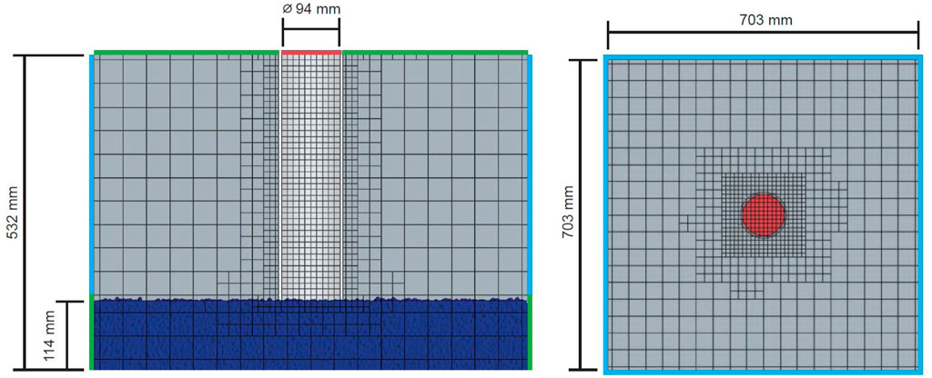
Figure 6. Numerical model of the vertical suction pipe test side view (left) and top view (right).
4 Results: single-phase (dry) calibration
Table 2 gives a summary of the general DEM input parameters used in the calibration simulations; in the case of input parameters that required calibration, the ranges of the evaluated values are given. The density of the particles was first calibrated by modelling a container filled with particles, and adjusting the particle solid density until the bulk density matched the measured value. Further calibration was conducted by systematically changing the input calibration parameters within the ranges specified. Since both the coefficient of restitution and the particle-particle coefficient of friction were identified as potential calibration parameters, the calibration sequence would need to include all combinations of these parameters within their respective ranges (full-factorial analysis).
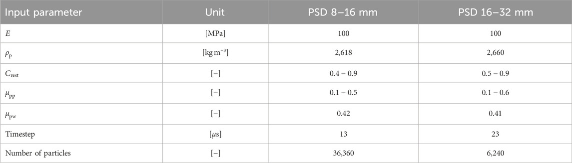
Table 2. General DEM input parameters and calibration ranges for single-phase (dry) conditions.
A series of tests were conducted for PSDs 8–16 mm and 16–32 mm. For each test, the final particle configuration was captured after the completion of the test and the respective angles extracted using automated image processing tools. As shown in Figure 3B, only the inner 70% of each respective profile was used in calculating the angles as this avoided the nonlinear regions at the extremities of the profiles. For both the shear angle and the angle of repose, the average between the two angles was used. The mass flow rate of each test was calculated by evaluating the slope of the mass change in the upper tank between 1 and 3 s after the start of material flow, as shown in Figure 3C.
A summary of the experimental test results is given in Table 3 under the heading “Dry Conditions”. Here the shear angle, angle of repose and mass flow rate are given by
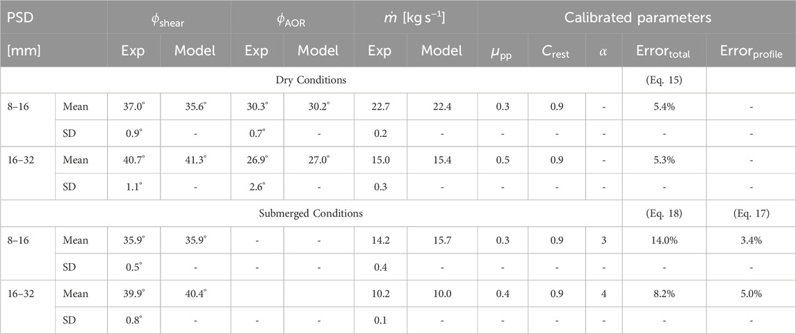
Table 3. Bulk property DDT results for the dry and submerged conditions respectively, including the experimental results, simulation results and the error, and the calibrated input parameter values.
An analysis was conducted to determine the sensitivity of the bulk material properties to changes in input parameters. The bulk material response was measured using the three characteristics described throughout, namely, the shear angle, angle of repose and mass flow rate. The results of the model’s sensitivity to changes to the particle-particle coefficient of friction and coefficient of restitution are outlined below. The model was found to be insensitive to changes in the particle elastic modulus.
Restitution coefficients of 0.4, 0.8, and 0.9 were implemented for the PSD 8–16 mm and 0.5, 0.7, 0.8, and 0.9 for PSD 16–32 mm, Figure 7 shows the modelled response for both PSDs. The shear angle was insensitivity to changes in the coefficient of restitution while the angle of repose decreased slightly with an increase in the restitution coefficient. The mass flow rate was somewhat sensitive to changes in the coefficient of restitution although no clear trend could be observed. Ye et al. (2018) conducted a sensitivity analysis on a DDT and determined the test to be insensitive to changes in the restitution coefficient, which contradicts the results shown here. The experimental DDT setup used by Ye et al. (2018) was significantly smaller than the test rig used here which meant a much shorter distance for particles to fall from the upper tank to the first contact surface. The sensitivity to changes in the coefficient of restitution, therefore, likely emerged as a result of the relatively high-velocity collisions of particles due to the large drop distance from the upper to the lower tank.
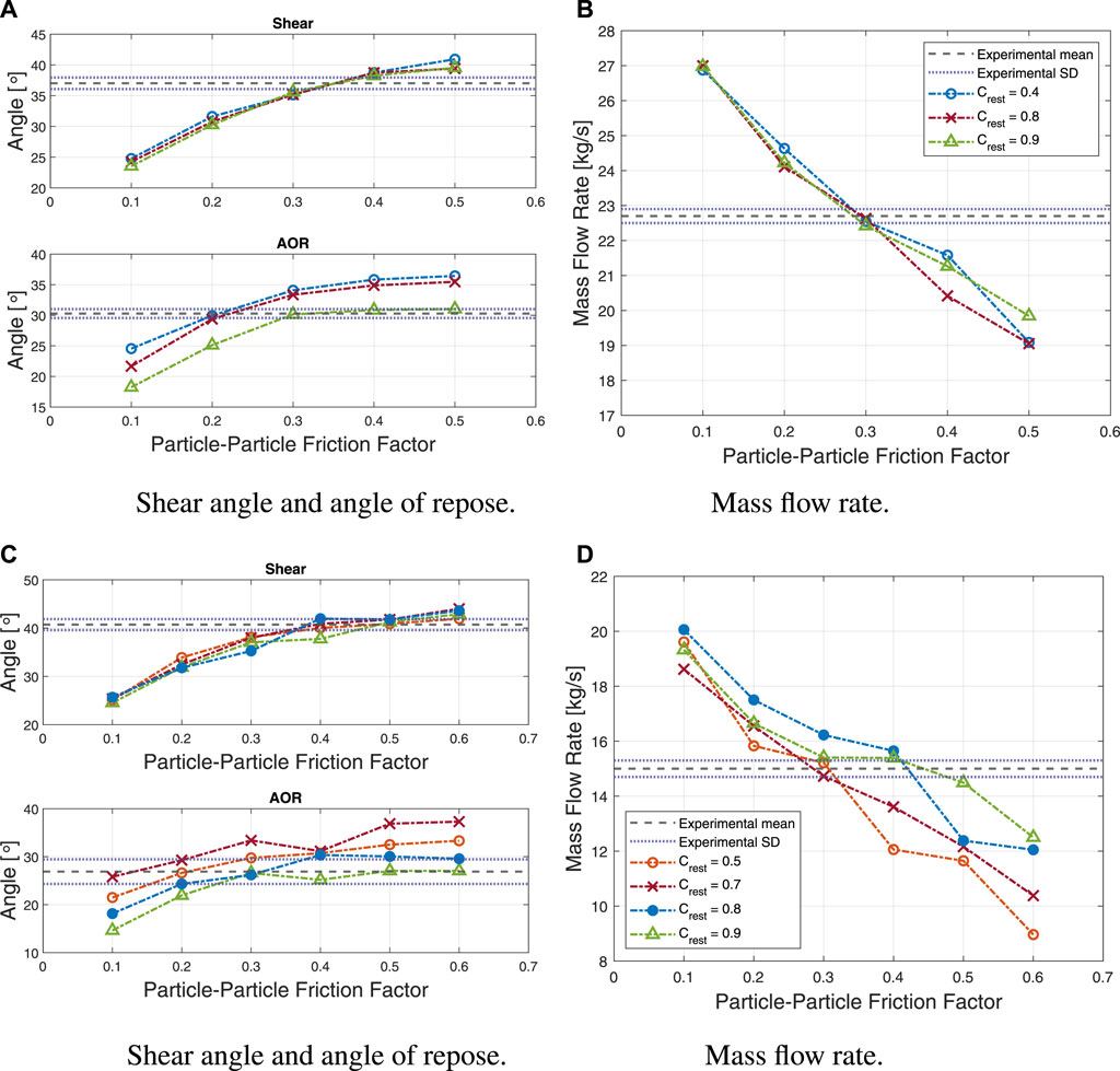
Figure 7. Calibration results under dry conditions showing the shear angle, angle of repose and the mass flow rate for for (A,B) PSD 8–16 mm and (C,D) PSD 16–32 mm (A). Shear angle and angle of repose (B). Mass flow rate (C). Shear angle and angle of repose (D). Mass flow rate.
To determine the sensitivity to changes in the particle-particle coefficient of friction, a range of 0.1–0.5 was used for PSD 8–16 mm and a range of 0.1–0.6 for PSD 16–32 mm, and the response of the bulk material measured as shown in Figure 7. Both the shear angle and the angle of repose are shown to be sensitive to changes in the coefficient of friction and showed an increase in angle as the friction increased. The mass flow rate decreased as the friction between particles increased. Similar trends were reported by Derakhshani et al. (2015), Coetzee (2016) and Roessler et al. (2019).
It is clear that some combinations of input parameters performed better than others when their results were evaluated against the experimental values. To disambiguate the potential calibration parameters, a total error for each combination of input parameters was calculated,
where
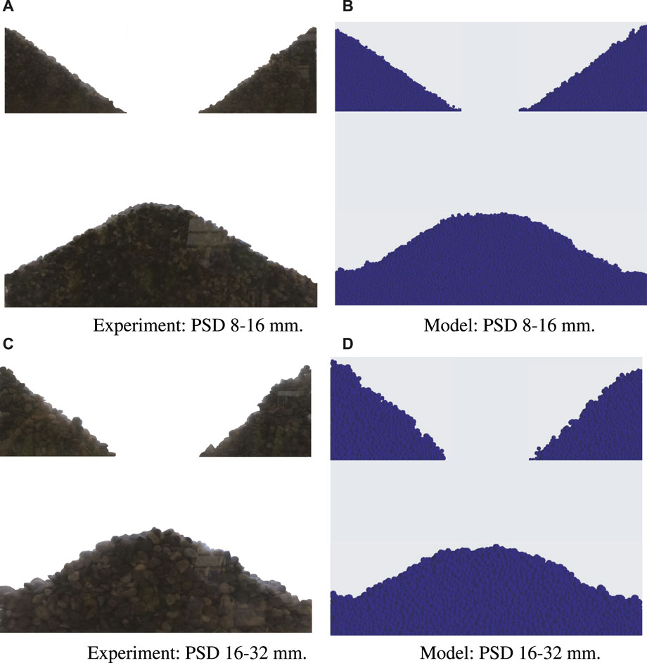
Figure 8. Final particle configuration in the single-phase (dry) experiment and model for (A,B) PSD 8–16 mm with calibrated parameters
5 Results: multiphase (submerged) calibration
5.1 Experiment
Figures 9, 10 show snapshots of submerged tests for PSDs 8–16 mm and 16–32 mm respectively (the timestamps refer to the time after the start of material flow). The addition of the fluid phase produced two observable effects that altered the response of the granular material when compared to the dry condition. Firstly, the maximum velocity of falling particles was significantly decreased due to the increase in drag and buoyancy forces. Secondly, induced fluid flow, caused by the column of falling particles, resulted in smaller particles being carried to the sides of the lower tank away from the main discharge column as seen in Figure 10B. This “mushrooming” effect resulted in a “double-bump” heap profile being formed in the lower tank for PSD 8–16 mm (Figure 10D), which meant that an angle of repose could no longer be defined or measured. On the other hand, the larger particles of PSD 16–32 mm resisted these effects and formed a profile similar to the ones seen in the dry tests, Figure 9D.
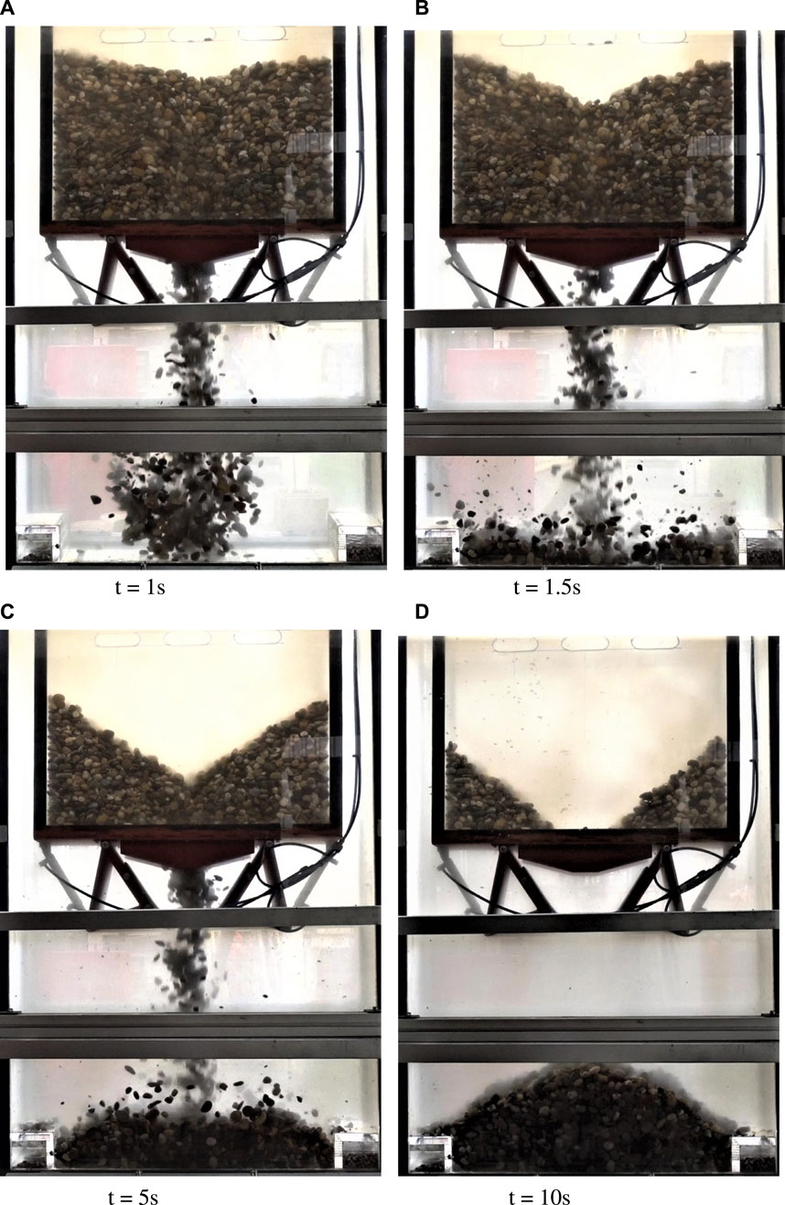
Figure 9. Submerged draw down test of PSD 16–32 mm at different times after start of flow (A). t = 1 s (B). t = 1.5 s (C). t = 5 s (D). t = 10 s.
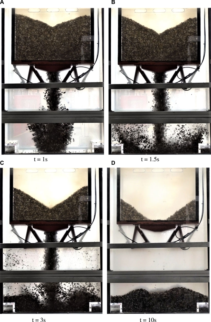
Figure 10. Submerged draw down test of PSD 8–16 mm at different times after start of flow (A). t = 1 s (B). t = 1.5 s (C). t = 3 s (D). t = 10 s.
Since an angle of repose could no longer be measured for PSD 8–16 mm, the entire profile of the heap that formed in the lower tank was extracted and used for calibration, including that of PSD 16–32 mm for consistency. However, the shear angle and mass flow rate could still be measured as in the dry tests, and the results are given in Table 3 under the heading “Submerged Conditions”.
It is clear that the submersion of the test rig greatly affected the mass flow rate of both PSDs which showed a significant decrease (32%–37%) when compared to the dry conditions. This is expected since the drag force resisted the flow of particles and significantly reduced their velocity. However, the difference in the shear angle between the submerged and dry conditions was very small (<1.1°) for both PSDs and statistically found to be insignificant (p
Images taken of the particle bed (heap) that formed in the lower tank were discretised and the height of the profile found at a number of points along its width. Figure 11A, for example, shows that the five repeated tests using PSD 16–32 mm produced very similarly shaped profiles and could be considered repeatable. A mean profile height and bounding region (minimum and maximum) were determined as shown in Figure 11B.
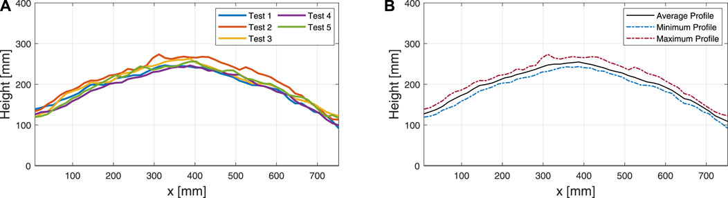
Figure 11. Height measurement of (A) DDT lower heap profiles from 5 repeated tests and (B) the averaged experimental profile and outer limits as a function of width (x).
5.2 Model
Table 4 summarises the CFD-DEM model parameters used in the multiphase simulations where range values are given for parameters that required calibration. The sensitivity of the model to the smoothing length, the drag coefficient (modifier) and the particle-particle coefficient of friction was investigated.
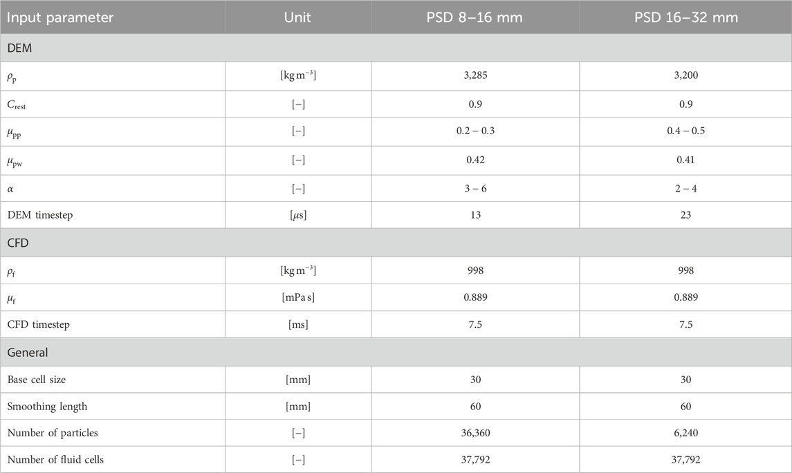
Table 4. General CFD-DEM input parameters and calibration ranges.
5.2.1 Source smoothing
The volume source smoothing method, described in Section 2.4, was employed to improve the stability of the CFD-DEM simulations with large particles. To explore the effects of source smoothing, a single particle with an equivalent sphere diameter of 32 mm was injected into the domain and allowed to fall (similar to the process followed by Song and Park (2020)). Figure 12 shows the particle velocity over time using smoothing lengths (cluster sizes) of 60 mm, 90 mm, and 120 mm, which resulted in cluster-to-particle ratios of 1.9, 2.8, and 3.8 respectively. The stability of the simulation increased with an increase in the smoothing length, as shown by the decrease in variation of the particle’s velocity from its terminal velocity (
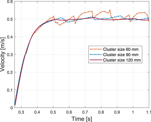
Figure 12. The effects of momentum source smoothing and cell clustering on particle velocity in a simple particle drop simulation.
Despite the increase in stability with increased smoothing lengths, other adverse effects emerged. When the smoothing length became large relative to the geometry of the fluid domain, particles could influence cells far removed from their position, significantly affecting the flow in these regions and interacting with boundaries where it should not. Therefore, the smoothing length should be chosen carefully to maximise stability and minimise the smearing effects. In this study a smoothing length of 60 mm (twice the base cell size) was implemented for both PSDs in the draw down tests.
5.2.2 Drag modifier
The drag force experienced by the particles as they move through the fluid phase is predominantly governed by the drag force model. A Haider-Levenspiel drag model Haider and Levenspiel (1989) was chosen since it considers the particle shape when determining the drag coefficient. The model, however, does not consider the effects of nearby particles, which can influence the drag experienced by a particle El-Emam et al. (2021). It was therefore decided that calibration of the drag coefficient would be required to account for these assumptions, simplifications, and the effects of source smoothing and cell clustering. A modified Haider-Levenspiel drag coefficient,
where
Using a PSD of 8–16 mm and the model inputs given in Table 4, the drag modifier was set to a value of 3, 4, 5, and 6 respectively, and the particle-particle coefficient of friction kept constant at 0.4. Figure 13A shows that the heap profile was sensitive to changes in the drag coefficient with the height decreasing in the centre of the heap directly below the upper tank opening, when the drag modifier was increased. This showed that an increase in the drag coefficient directly affected the magnitude of fluid-particle interaction with an increased number of particles carried further away from the centre of the tank. Figure 13B shows the shear angle was not sensitive to changes in the drag coefficient, while as expected, there was a significant decrease in the mass flow rate with an increase in the drag coefficient.
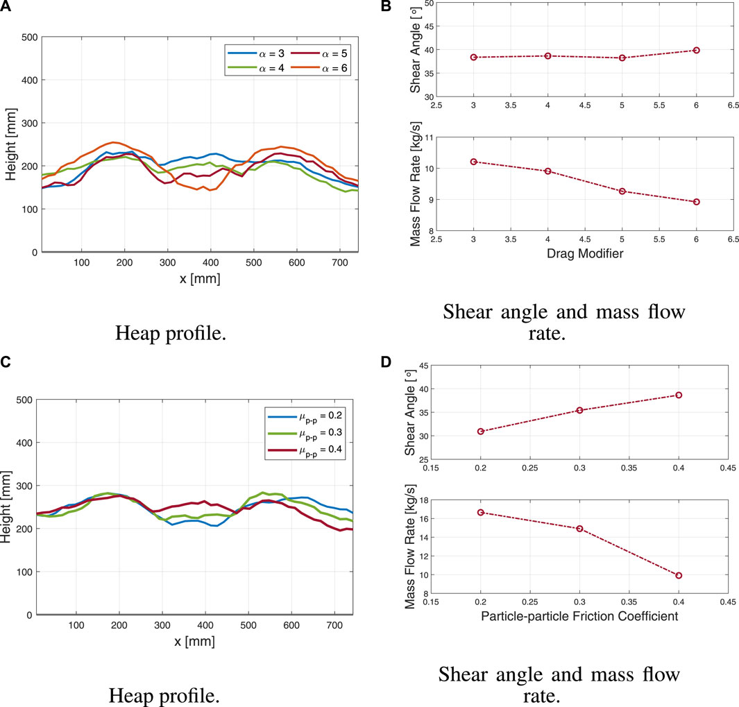
Figure 13. Sensitivity of the heap profile, the shear angle and the mass flow rate to (A,B) changes in the drag coefficient modifier and (C,D) changes in the particle-particle coefficient of friction (A). Heap profile (B). Shear angle and mass flow rate (C). Heap profile (D). Shear angle and mass flow rate.
5.2.3 Particle-particle friction
Particle-particle coefficients of friction of 0.2, 0.3, and 0.4 were implemented with a constant drag coefficient modifier of 4. Figures 13C,D show all three bulk properties to be sensitive to changes in the friction with an increase in the shear angle and a decrease in the mass flow rate when the friction was increased. The heap profile was sensitive to changes in the friction, but less sensitive compared to changes in the drag coefficient. The height of the profile at the centre of the tank increased with an increase in the friction.
5.3 Calibration results
A calibration procedure was conducted wherein the drag coefficient modifier and particle-particle coefficient of friction were calibrated for both PSDs under submerged conditions. The modelled shear angles, mass flow rates and heap profiles were compared to the experimental measurements to identify a parameter set with the lowest total error.
The heap profile was measured using the same technique as described in Section 5.1 and used alongside the measured shear angle and mass flow rate to determine the model accuracy. The error in the modelled heap profile was calculated as,
where
where
5.3.1 PSD 16–32 mm
Drag coefficient modifiers of 2, 3, and 4 were implemented along with particle-particle coefficients of friction of 0.4 and 0.5, where 0.5 was the calibrated coefficient of friction found during the dry calibration procedure (Section 4). The parameter combination
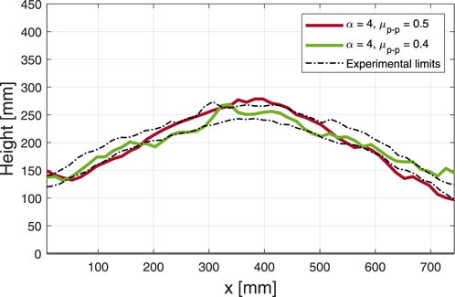
Figure 14. Submerged repose profiles for PSD 16–32 mm using
Figure 15 compares the final particle configuration of the experiment and a simulation with input parameters of
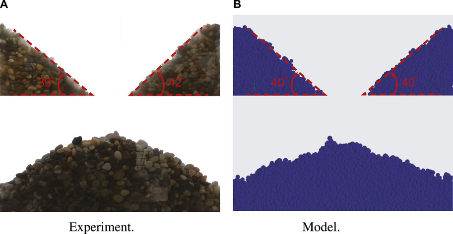
Figure 15. Shear angles and repose profiles of the (A) experiment and (B) calibrated model with
5.3.2 PSD 8–16 mm
A drag modifier range of 3–6 was implemented with particle-particle coefficients of friction of 0.2 and 0.3, where 0.3 was the calibrated coefficient found during the dry calibration procedure (Section 4).
The parameter combination
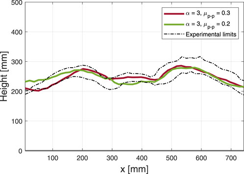
Figure 16. Submerged repose profiles for PSD 8–16 mm using
A friction coefficient of 0.2 failed to accurately predict the shear angle and mass flow rate over the whole range of drag modifiers tested. As with the PSD 16–32 mm, the coefficient of friction,
6 Model verification: vertical suction pipe
The general model input parameters of the vertical suction pipe simulations are given in Table 5.
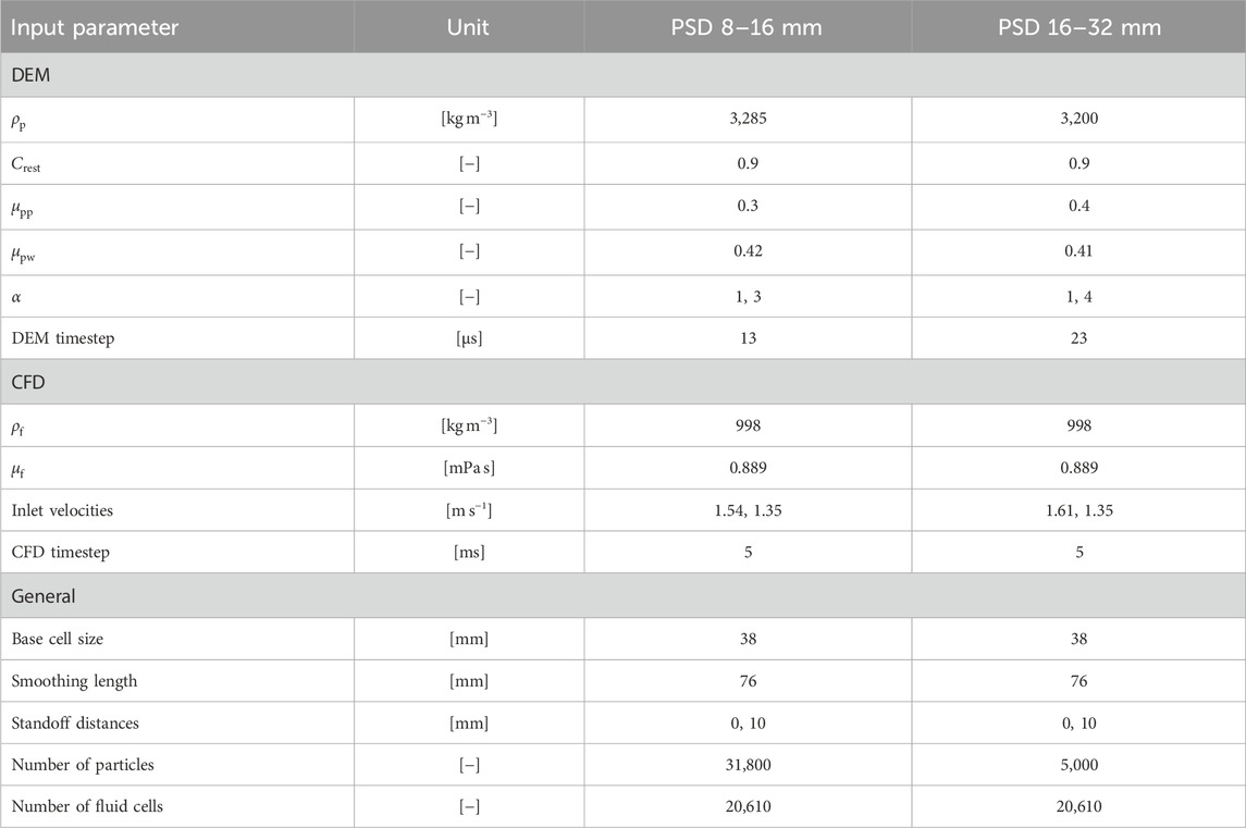
Table 5. General CFD-DEM input parameters used for validation.
6.1 Results
The results of the various test configurations are summarised in Table 6. The removed mass and the cavity depth and diameter were sensitive to changes in the standoff distance and fluid velocity and, as expected, increased as the standoff distance was decreased or the fluid velocity was increased.
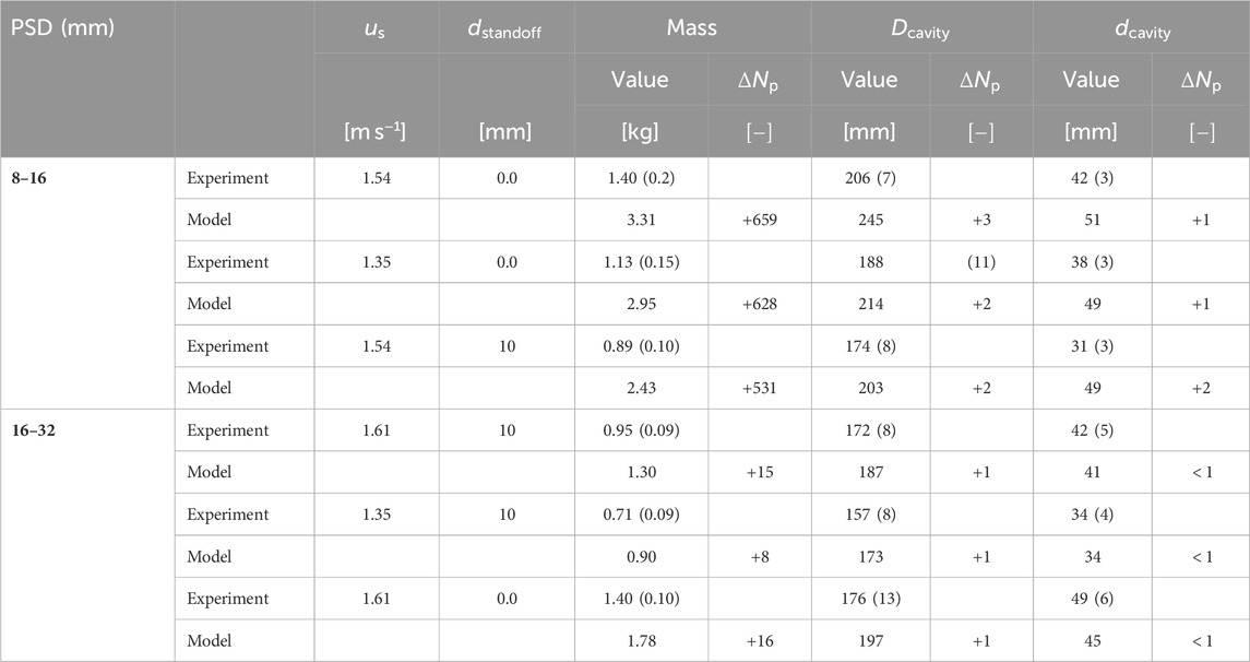
Table 6. Vertical suction pipe experimental (mean value and standard deviation in brackets) and simulation results using calibrated input parameters.
Table 6 compares the modeled and experimental results of both PSDs. Due to the discreet nature of particulate systems, the removal of one or two additional particles can significantly influence the results in terms of the mass removed and the diameter and depth of the cavity. Thus, besides reporting the actual values, the error in the prediction of the mass removed, and the cavity diameter and depth is also expressed in terms of the number of particles,
The model exhibited the correct trends when the test configuration was changed, namely, an increase in the removed mass, cavity diameter and cavity depth as the standoff distance decreased or the pipe velocity increased. A general increase in these three measures when the size of the particles decreased, was also correctly predicted.
The model over-predict the removed mass and cavity size for both PSDs and all test configurations. However, due to the small ratio of cavity depth and diameter to average particle diameter, the over-prediction of cavity size was still accurate to within three particle diameters,
6.2 Model sensitivity
The suction pipe experiment was done for validation, and although the model could accurately predict the cavity size, it could not accurately predict the removed mass. To better understand this, and to identify why the calibration process failed at this aspect, the suction pipe model was subjected to a sensitivity study where the particle-particle coefficient of friction and the drag coefficient (modifier) was varied.
6.2.1 Particle friction
Particle-particle friction coefficients of 0.4, 0.5, and 0.6 were implemented for the 16–32 mm PSD without a drag modifier
6.2.2 Drag coefficient
With the suction pipe model insensitive to the particle-particle coefficient of friction, the only parameter that could be reasonably adjusted was the coefficient of drag. A series of simulations was conducted wherein drag modifiers of 1, 2, and 4 were implemented with the 16–32 mm PSD, and a test configuration with
Figure 17 shows that the three measures were sensitive to changes in the drag modifier and increased with an increase in the drag modifier. This confirms that the over-prediction seen for the models using calibrated drag modifiers was due to the high modifier values and shows that the model prediction could be improved if the drag modifier values were to be decreased.

Figure 17. Influence of the drag modifier on the displaced mass and the cavity diameter and depth.
In the DDT calibration model, there was initially a lack of fluid-particle interaction which is the reason why the drag modifier was introduced as the only feasible means of obtaining accurate calibration results. However, in the model of the suction pipe the lack of interaction was not observed and removing the drag modifier (setting
7 Conclusion
Fluid-particle systems are integral to many industrial and natural processes and exhibit complex behaviours which make these systems difficult to model and predict. Calibration is a critical component in the accurate modelling of these systems, but calibration practices have been mostly limited to single-phase environments. To better understand the effects that fluid-particle interaction has on input parameters, a multi-phase calibration method was devised. Two particle size distributions (PSDs) were calibrated using draw down tests (DDTs), allowing both the particle coefficient of restitution and the particle-particle coefficient of friction to be successfully calibrated for single-phase (dry) conditions.
The DDTs were repeated for submerged conditions and the changes in material behaviour were observed. The shear angles in the upper tank of the DDT were unaffected by the submerged condition. A fully coupled CFD-DEM model of the DDT was constructed and source smoothing was implemented to accommodate particles larger than the mesh size and to increase the stability of the model. A drag coefficient modifier was added as an additional calibration parameter and calibrated along with the particle-particle coefficient of friction.
A vertical suction pipe experiment was conducted on particle beds of the same PSDs to validate the calibrated input parameters using three distinct test configurations of pipe velocity and standoff distance. The lack of fluid-particle interaction seen in the submerged DDT was not found in the vertical suction simulation which resulted in an over-prediction of the measured properties.
The submerged calibration procedure showed that particle-particle coefficient of friction calibrated in a single-phase environment could be reliably implemented into multi-phase applications, without any modification. The drag modifier was identified as a necessary calibration parameter for the submerged DDT simulation due to the presence of momentum source smoothing and cell clustering effects that reduced the fluid-particle interaction in this particle-driven flow environment. However, in the suction pipe simulation the calibrated drag modifiers overestimated the fluid-particle interaction in a fluid-driven environment. It is concluded that due to the difference in flow environment (particle versus fluid driven), the DDT experiment is not well-suited for calibrating the input parameters used in suction pipe modelling. It is advised that the flow environment in the calibration test should be similar to that in the validation test or final application.
Further research is needed to understand the limitations of calibrated CFD-DEM input parameters for multi-phase applications. It is unknown to what extent the calibrated drag modifier is dependent on the conditions of the fluid domain and what effects changes to the fluid domain, such as cell size, smoothing length and boundary conditions would have on the performance of the parameters. The effects of source smoothing also require further investigation, especially within the context of particle-driven flow versus fluid-driven flow.
Data availability statement
The raw data supporting the conclusions of this article will be made available by the authors, without undue reservation.
Author contributions
JW: Conceptualization, Formal Analysis, Methodology, Validation, Writing–original draft. CC: Conceptualization, Funding acquisition, Methodology, Supervision, Writing–review and editing. CM: Conceptualization, Methodology, Supervision, Writing–review and editing.
Funding
The author(s) declare that financial support was received for the research, authorship, and/or publication of this article. Funding towards this research project was provided by De Beers Marine (Pty) Ltd.
Conflict of interest
The authors declare that the research was conducted in the absence of any commercial or financial relationships that could be construed as a potential conflict of interest.
Publisher’s note
All claims expressed in this article are solely those of the authors and do not necessarily represent those of their affiliated organizations, or those of the publisher, the editors and the reviewers. Any product that may be evaluated in this article, or claim that may be made by its manufacturer, is not guaranteed or endorsed by the publisher.
Supplementary material
The Supplementary Material for this article can be found online at: https://www.frontiersin.org/articles/10.3389/fceng.2024.1376974/full#supplementary-material
References
Akhshik, S., Behzad, M., and Rajabi, M. (2016). Simulation of the interaction between nonspherical particles within the CFD–DEM framework via multisphere approximation and rolling resistance method. Part. Sci. Technol. 34, 381–391. doi:10.1080/02726351.2015.1089348
Bravo-Blanco, A., Sánchez-Medina, A., and Ayuga, F. (2017). Analysis of the incipient motion of spherical particles in an open channel bed, using a coupled computational fluid dynamics–discrete element method model. Biosyst. Eng. 155, 68–76. doi:10.1016/j.biosystemseng.2016.12.003
Chen, J., Nishiura, D., and Furuichi, M. (2021). DEM study of the influences of the geometric and operational factors on the mechanical responses of an underwater mixing process. Powder Technol. 392, 251–263. doi:10.1016/j.powtec.2021.06.049
Coetzee, C. (2016). Calibration of the discrete element method and the effect of particle shape. Powder Technol. 297, 50–70. doi:10.1016/j.powtec.2016.04.003
Coetzee, C. (2020). Calibration of the discrete element method: strategies for spherical and non-spherical particles. Powder Technol. 364, 851–878. doi:10.1016/J.POWTEC.2020.01.076
Coetzee, C. J. (2017). Review: calibration of the discrete element method. Powder Technol. 310, 104–142. doi:10.1016/j.powtec.2017.01.015
Cundall, P. A., and Strack, O. D. L. (1979). A discrete numerical model for granular assemblies. Geotechnique 29, 47–65. doi:10.1680/geot.1979.29.1.47
Derakhshani, S. M., Schott, D. L., and Lodewijks, G. (2015). Micro-macro properties of quartz sand: experimental investigation and DEM simulation. Powder Technol. 269, 127–138. doi:10.1016/j.powtec.2014.08.072
El-Emam, M. A., Zhou, L., Shi, W., Han, C., Bai, L., and Agarwal, R. (2021). Theories and applications of CFD–DEM coupling approach for granular flow: a review. Archives Comput. Methods Eng. 28, 4979–5020. doi:10.1007/s11831-021-09568-9
Feng, Y. T. (2023). Thirty years of developments in contact modelling of non-spherical particles in DEM: a selective review. Acta Mech. Sin. 39, 722343. doi:10.1007/s10409-022-22343-x
Gao, X., Shi, W., Shi, Y., Chang, H., and Zhao, T. (2020). DEM-CFD simulation and experiments on the flow characteristics of particles in vortex pumps. Water 12, 2444–2461. doi:10.3390/w12092444
Govender, N. (2021). Study on the effect of grain morphology on shear strength in granular materials via GPU based discrete element method simulations. Powder Technol. 387, 336–347. doi:10.1016/j.powtec.2021.04.038
Govender, N., Kobyłka, R., and Khinast, J. (2023). The influence of cohesion on polyhedral shapes during mixing in a drum. Chem. Eng. Sci. 270, 118499. doi:10.1016/j.ces.2023.118499
Guo, Y., and (Bill) Yu, X. (2017). Comparison of the implementation of three common types of coupled cfd-dem model for simulating soil surface erosion. Int. J. Multiph. Flow 91, 89–100. doi:10.1016/j.ijmultiphaseflow.2017.01.006
Haider, A., and Levenspiel, O. (1989). Drag coefficient and terminal velocity of spherical and nonspherical particles. Powder Technol. 58, 63–70. doi:10.1016/0032-5910(89)80008-7
He, L., Liu, Z., and Zhao, Y. (2024). Study on a semi-resolved CFD-DEM method for rod-like particles in a gas-solid fluidized bed. Particuology 87, 20–36. doi:10.1016/j.partic.2023.07.014
Hertz, H. (1881). Über die Berührung fester elastischer Körper. J. für die reine und angewandte Math. 92, 156–171.
Hesse, R., Krull, F., and Antonyuk, S. (2020). Experimentally calibrated CFD-DEM study of air impairment during powder discharge for varying hopper configurations. Powder Technol. 372, 404–419. doi:10.1016/j.powtec.2020.05.113
Jaiswal, A., Bui, M. D., and Rutschmann, P. (2024). On the process of fine sediment infiltration into static gravel bed: a cfd–dem modelling perspective. River Res. Appl. 40, 29–48. doi:10.1002/rra.4215
Jing, L., Yang, G. C., Kwok, C. Y., and Sobral, Y. D. (2019). Flow regimes and dynamic similarity of immersed granular collapse: a CFD-DEM investigation. Powder Technol. 345, 532–543. doi:10.1016/j.powtec.2019.01.029
Lavrinec, A., Orozovic, O., Rajabnia, H., Williams, K., Jones, M. G., and Klinzing, G. (2020). Velocity and porosity relationships within dense phase pneumatic conveying as studied using coupled CFD-DEM. Powder Technol. 375, 89–100. doi:10.1016/j.powtec.2020.07.070
Lu, R., Luo, Q., Wang, T., and Zhao, C. (2022). Comparison of clumps and rigid blocks in three-dimensional DEM simulations: curvature-based shape characterization. Comput. Geotechnics 151, 104991. doi:10.1016/j.compgeo.2022.104991
Marigo, M., and Stitt, E. H. (2015). Discrete element method (DEM) for industrial applications: comments on calibration and validation for the modelling of cylindrical pellets. Powder Technol. 32, 236–252. doi:10.14356/kona.2015016
Mindlin, R. D. (1949). Compliance of elastic bodies in contact. J. Appl. Mech. 16, 259–268. doi:10.1115/1.4009973
Mindlin, R. D., and Deresiewicz, H. (1953). Elastic spheres in contact under varying oblique forces. J. Appl. Mech. 20, 327–344. doi:10.1115/1.4010702
Radvilaitė, U., Ramírez-Gómez, Á., and Kačianauskas, R. (2016). Determining the shape of agricultural materials using spherical harmonics. Comput. Electron. Agric. 128, 160–171. doi:10.1016/j.compag.2016.09.003
Roessler, T., Richter, C., Katterfeld, A., and Will, F. (2019). Development of a standard calibration procedure for the DEM parameters of cohesionless bulk materials – part I: solving the problem of ambiguous parameter combinations. Powder Technol. 343, 803–812. doi:10.1016/j.powtec.2018.11.034
Rossow, J., and Coetzee, C. J. (2021). Discrete element modelling of a chevron patterned conveyor belt and a transfer chute. Powder Technol. 391, 77–96. doi:10.1016/j.powtec.2021.06.012
Song, S., and Park, S. (2020). Unresolved cfd and dem coupled solver for particle-laden flow and its application to single particle settlement. J. Mar. Sci. Eng. 8, 983–1021. doi:10.3390/jmse8120983
Vallejo, L. E., Espitia, J. M., and Caicedo, B. (2017). The influence of the fractal particle size distribution on the mobility of dry granular materials. EPJ Web Conf. 140, 03032. doi:10.1051/epjconf/201714003032
Versteeg, H. K., and Malalasekera, W. (2007). An introduction to computational fluid dynamics: the finite volume method. Harlow, England: Pearson Education Ltd.
Wang, Z., Teng, Y., and Liu, M. (2019). A semi-resolved CFD-DEM approach for particulate flows with kernel based approximation and Hilbert curve based searching strategy. J. Comput. Phys. 384, 151–169. doi:10.1016/j.jcp.2019.01.017
Wensrich, C. M., and Katterfeld, A. (2012). Rolling friction as a technique for modelling particle shape in DEM. Powder Technol. 217, 409–417. doi:10.1016/j.powtec.2011.10.057
Wensrich, C. M., Katterfeld, A., and Sugo, D. (2014). Characterisation of the effects of particle shape using a normalised contact eccentricity. Granul. Matter 16, 327–337. doi:10.1007/s10035-013-0465-1
Ye, F., Wheeler, C., Chen, B., Hu, J., Chen, K., and Chen, W. (2018). Calibration and verification of DEM parameters for dynamic particle flow conditions using a backpropagation neural network. Adv. Powder Technol. 30, 292–301. doi:10.1016/j.apt.2018.11.005
Yuan, F.-L. (2024). Sr-dem: an efficient discrete element method for particles with surface of revolution.
Zhang, J., Li, T., Ström, H., Wang, B., and Løvås, T. (2023). A novel coupling method for unresolved CFD-DEM modeling. Int. J. Heat Mass Transf. 203, 123817. doi:10.1016/j.ijheatmasstransfer.2022.123817
Zhou, H., Wang, G., Jia, C., and Li, C. (2019). A novel, coupled CFD-DEM model for the flow characteristics of particles inside a pipe. WaterSwitzerl. 11, 2381. doi:10.3390/w11112381
Keywords: CFD-DEM, draw down test, submerged, calibration, suction pipe
Citation: Wasserfall JG, Coetzee CJ and Meyer CJ (2024) A submerged draw down test calibration method for fully-coupled CFD-DEM modelling. Front. Chem. Eng. 6:1376974. doi: 10.3389/fceng.2024.1376974
Received: 26 January 2024; Accepted: 13 June 2024;
Published: 12 July 2024.
Edited by:
Alejandro López, University of Deusto, SpainReviewed by:
Alberto Di Renzo, University of Calabria, ItalyFrancisco Ayuga, Polytechnic University of Madrid, Spain
Copyright © 2024 Wasserfall, Coetzee and Meyer. This is an open-access article distributed under the terms of the Creative Commons Attribution License (CC BY). The use, distribution or reproduction in other forums is permitted, provided the original author(s) and the copyright owner(s) are credited and that the original publication in this journal is cited, in accordance with accepted academic practice. No use, distribution or reproduction is permitted which does not comply with these terms.
*Correspondence: Corné J. Coetzee, ccoetzee@sun.ac.za