Non-invasive rust detection of steel plates determined through interfacial modulus

Initial methods to detect rust in pipelines have been conducted through invasive probes and sectioning off parts of the facility as the plant is running. These methods greatly increase the costs overall. The need for a feasible solution to this issue lies in the detection of rust formation through a non-invasive method. This study’s objective is to measure rust formation through droplet motion on the outer layer of pipelines. Multiple experiments are conducted using carbon steel sheets whose bottom layer has been exposed to acid for different durations of time. As rust formation in the metal is a voltaic phenomenon, it would mean that the acid corrosion of the bottom layer would adversely affect the top layer of the substrate. Consequentially, droplet motion and the droplet’s contour would change in different corrosive scenarios which we could then detect with novel parameters in our lab. One such parameter is the Interfacial Modulus (G_S), which describes the initial resistance of the solid’s outer layer towards the liquid. We can understand this parameter with the aid of the novel device, known as the Centrifugal Adhesion Balance (CAB). As we cause the drop to slide across the substrate at constant normal force condition, we observe the difference in the contour of the drop as it slides across the substrate. The real-time change in contact angles at each edge of the drop, along with its change in external lateral force, causes a change in the G_S values, which varies in different corrosive scenarios.

1 Introduction

Corrosion, also known as rust in the case of iron and steel, is the gradual degradation of a material through chemical reactions with its environment. Corrosion can cause structural damage, reduce the functional lifespan of an object, and even lead to failure in critical systems. Corrosion is a natural process in which a refined metal tries to attend its more chemically stable form such as oxide, hydroxide, carbonate, or sulfide. In other words, it is a gradual destruction of materials (usually by chemical or electrochemical reaction of metals with its environment) .

The importance of understanding corrosion and rust lies in its pervasive impact on infrastructure, buildings, vehicles, and equipment. The economic costs of corrosion can be significant, resulting in reduced efficiency, increased maintenance costs, and shortened lifespans of equipment and infrastructure.

Moreover, corrosion can pose significant safety risks in various industries, including aviation, transportation, and chemical processing. For example, a corroded aircraft part or bridge component can fail unexpectedly, leading to catastrophic accidents.

In the context of the environment, corrosion can also lead to pollution of soil and water resources through the release of chemicals used in corrosion protection and cleaning.

Therefore, understanding the mechanisms of corrosion and implementing effective prevention and mitigation strategies is critical to maintaining the reliability, safety, and longevity of infrastructure and equipment, as well as protecting the environment.

According to National Association of Corrosion Engineering (NACE), they conducted a study in 2002 for obtaining the data and see the impact of corrosion on United States. economy and estimated that the total cost of the corrosion in United States is approximately 276 billion USD (which is 3.1% of Nation’s GDP at that time) (Koch et al., 2002).

Current instruments and techniques for detecting corrosion and rust include visual inspection, ultrasonic inspection, electrochemical techniques, and non-destructive testing methods. These methods have varying degrees of effectiveness and are often used in combination to provide a more comprehensive assessment of corrosion damage.

Visual inspection is a straightforward method of detecting corrosion but is limited to surface rust that is visible to the naked eye. Ultrasonic inspection uses high-frequency sound waves to detect corrosion and is useful for detecting rust and corrosion in areas that are difficult to access. Electrochemical techniques, such as corrosion potential and polarization measurements, are used to assess the rate of corrosion and predict its progression. Non-destructive testing methods, such as X-ray diffraction and magnetic particle testing, are used to detect hidden corrosion.

However, each of these techniques has its limitations. For example, visual inspection is limited to surface corrosion, and ultrasonic inspection may not be effective in detecting rust that is hidden under thick coatings or in hard-to-reach areas. Electrochemical techniques require a good understanding of the materials and conditions under investigation, and non-destructive testing methods may require specialized equipment and trained personnel.

Once the metal comes in its working environment it is subjected to flaws, deterioration, and loss in many other forms. Among all the corrosion is particularly the most significant threat to all the industries as it weakens the entire structure which may lead to an irreplaceable damage to the structure if the corrosion is not monitored/detected ahead of time. Hence, it was desirable to develop a technique to detect the rust formation in metal at early stage so that we can run all the preventive measures and metal can be protected.

One of the biggest challenges in the field of corrosion prevention and control is detecting rust formation in its early stages. If left undetected, rust can continue to spread and cause significant damage to equipment and infrastructure. It is therefore essential to develop effective methods for detecting rust in its earliest stages.

Therefore, developing new, more sensitive and specific techniques for detecting early-stage rust formation and corrosion is crucial to preventing and mitigating the effects of corrosion. Researchers are exploring the use of advanced imaging techniques, such as optical coherence tomography and scanning electron microscopy, to detect corrosion at a microscopic level. Other areas of research include the development of smart coatings and materials that can detect corrosion and self-heal, as well as the use of artificial intelligence and machine learning algorithms to detect corrosion patterns and predict the progression of corrosion damage.

Since rust formation occurs when iron or steel is exposed to oxygen and water, and the wetting properties of such metals can influence the formation and growth of rust, we propose studying wetting properties to detect rust formation. We study this by utilizing Centrifugal Adhesion Balance (CAB) to evaluate the interfacial modulus (G_S), which represents the resistance of the solid layer to interact with the given liquid. This can solve the issue of detecting corrosion through a non-invasive method which will mitigate the high costs that could occur when using isolation or UV probe methods. In addition, our proposed method can increase profit and lead to continuous monitoring of corrosion levels without compromising or exposing the pipelines to any leaks that may occur through a non-invasive method. It can also inspire further research, where wetting characterization methods, such as contact angle measurements and force-based techniques, could be utilized to detect early rust formation on various metals and coatings.

2 Interfacial modulus for quantitative description of rust formation

For our study, we will be using the same surface property (i.e., Interfacial modulus or G_S) proposed by Tadmor to assess the development of corrosion on the inner wall of the given metal. In our work, we are using Centrifugal Adhesion Balance (CAB) [Tadmor et al., PRL 103, 266101 (2009)] to assess the development of corrosion from the inner to the outer wall of the given metal by measuring interfacial modulus (G_S). More precisely, we are probing the change in wetting properties, which are a consequence of corrosion.

2.1 Concept and fundamental theory of interfacial modulus

Interfacial Modulus $G_S$, is the microscopic property of solid surface molecules to re-orient the functional groups within its outer layer. The solid molecules may protrude towards liquid from their buried position or vice versa (Yadav et al., 2018), which can be seen from Figure 1.

FIGURE 1

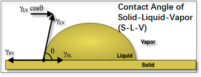
FIGURE 1. Representing two-dimensional figure of a liquid drop resting on solid surface with their surface tensions on the triple point ( ${\gamma }_{SV}$ is the solid-vapor surface tension; ${\gamma }_{SL}$ is the solid-liquid surface tension; ${\gamma }_{LV}$ is the liquid-vapor surface tension; $\theta$ is the thermodynamic equilibrium contact angle) (Yadav et al., 2018; Young, 1805; Tadmor, 2021; Tadmor, 2013; Tadmor, 2011; Tadmor, 2004; Tadmor et al., 2009; N’guessan et al., 2012; Wasnik et al., 2015; Tadmor et al., 2008; Yadav et al., 2008).

The first well known study in the field of Surface Science on the wetting phenomena was done about two centuries back in 1805 by Thomas Young (Young, 1805). The mathematical relation given by him in his study is the vectorial summation of the surface tensions in the lateral direction which relates the drop’s thermodynamic equilibrium contact angle with the surface forces which was first written by Dupré (Dupré and Dupré, 1869) as follows:

$\mathit{cos}\theta =\frac{{\gamma }_{SV}-{\gamma }_{SL}}{{\gamma }_{LV}}(1)$

where, ${\gamma }_{SV}$ is the solid-vapor surface tension, ${\gamma }_{SL}$ is the solid-liquid surface tension, ${\gamma }_{LV}$ is the liquid-vapor surface tension and $\theta$ is the thermodynamic equilibrium contact angle.

However, Young’s equation has several limitations; firstly, it is only valid for solid which is perfectly homogeneous, smooth, rigid and in its thermodynamically idealized state (Lester, 1961; Rusanov, 1975; Pethica, 1977; Shanahan et al., 1987; Carré et al., 1996; Meiron et al., 2004); secondly, it does not include the resilience of solid layer to interact with given liquid. Therefore, Equation 1 is not considered for contact angle hysteresis, pinning, or retention force. In real scenarios there is no such solid which is perfectly homogenous, smooth, and rigid, there is always some kind of deformation in the solid which this equation does not consider and so its application is minimal. Usually, there are some small protrusions of solid (shown by Shanahan and de Gennes (Shanahan and Degennes, 1986; Shanahan et al., 1987) and by Butt et al. (Butt et al., 2018)), due to which it will cause less resilience and interacts with the given liquid to maximum extent and cause liquid droplet to move on solid layer. The relation to the resilience can be given by the interfacial modulus (G_S), obtained by combining Shanahan, de Gennes and Tadmor’s approach. Interfacial modulus represents the resistance of solid layer to interact with the given liquid.

The greater the interaction between solid surface and liquid the lower will be the Gs value and vice versa as the solid molecules will reorient itself when it interacts with the given liquid and the protrusions are created on the solid layer. For the surface, which is relatively free of blemishes (Shanahan et al., 1987; Tadmor, 2021), the equation proposed by Tadmor for interfacial modulus (G_S) is as follows (Tadmor, 2013; Tadmor, 2021):

$G_S=\frac{4{{\gamma }_{LV}}^2\mathit{sin}\theta }{f_{\parallel }}\left(cos{\theta }_R-\mathit{cos}{\theta }_A\right)(2)$

where $G_S$ is the interfacial modulus, $f_{\parallel }$ is the lateral force, ${\gamma }_{LV}$ is the liquid-vapor surface tension, $\theta$ is the apparent contact angle, ${\theta }_R$ is the receding contact angle and ${\theta }_A$ is the advancing contact angle.

2.2 Centrifugal Adhesion Balance (CAB)

Centrifugal Adhesion Balance (CAB) is a novel instrument constructed in the Surface Science Lab, Lamar University (Tadmor, 2021; Tadmor, 2013; Tadmor, 2011; Tadmor, 2004; Tadmor et al., 2009; N’guessan et al., 2012; Wasnik et al., 2015; Tadmor et al., 2008; Yadav et al., 2008).

The idea of CAB comes from the idea to study 1) Wettability–the ability of a liquid to maintain contact with a solid surface, 2) Solid Liquid tribology–the stress induced by the two media in contact with one another and in opposite motion, i.e., retention or friction, 3) Retention work–related to the field of tribology, which helps us understand how the solid interacts/resists the interaction to the given liquid that is sliding across it, 4) Work of adhesion–helps us understand the physical nature of solid-liquid system, specifically the solid, by analyzing the ‘flying’ detachment of the liquid from the surface.

The Goniometers are the one of the common methods to measure the contact angle, but they might suffer from contact angle hysteresis which may results in different measurement depending on the surface roughness, surface homogeneities, even the height from which the droplet ejected. As this method has so many contingencies, there was a need to determine a new method. So, the next method was created to make a tilting stage effect, in which the drop was subjected to an incline at a given angle. Though this method is better than the previous one, however it suffers from one issue, the normal force, and the lateral force work together on the droplet. This means that, there are two independent variables working in the experimental run which defeats the very essence of experiment.

CAB allows independent manipulation of lateral force and the normal force, unlike the conventional tilt-stage method in which it was very difficult to manipulate the normal force and the lateral force independently (Tadmor, 2011; Tadmor, 2013; Tadmor, 2021). As in CAB, the drop motion is induced by centrifugal force while the gravitational force is the driving force for drop motion in the conventional tilt-stage method.

The CAB is made up of one rotating arm (inside Item 1 in Figure 2) which rotates perpendicular to the gravitational field. The schematic of the CAB is shown in Figure 2. There is one control box (Item 2 in Figure 2) which has connection to camera and receives signal from the camera and then transfer it wirelessly to the external computer situated near the rotating assembly setup. On one end of the rotating arm there is a plate on which the camera, source of light and clamps to hold the substrate are attached while on the other end there is a counterbalance attached (Item 3 in Figure 2). The position of the plate is fixed with respect to the rotating arm, but the tilt of the plate can be varied at any angle from 0° to 360°. The DC motor (Item 4 in Figure 2) is connected to the round disc on the shaft which touches the encoder and the Encoder (Item 5 in Figure 2) is used to monitor the angular velocity.

FIGURE 2

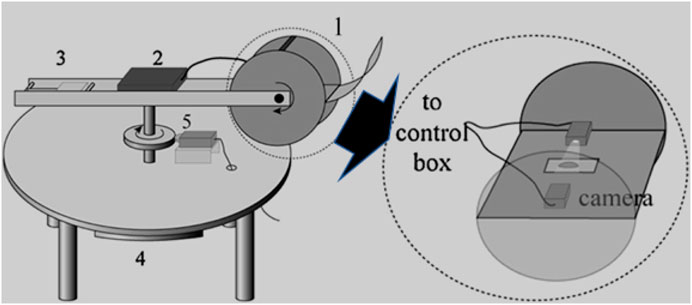
FIGURE 2. Prototype of Centrifugal Adhesion Balance (first-generation) (1) Closed chamber - on one of the ends of rotating arm which contains a sample holder in between camera and light source (2) Control box - connected to camera and receives signal from the camera and transfer it wirelessly to the external computer situated near the rotating assembly setup. (3) Counterbalance–on another end of rotating arm (4) DC motor connected to the round disc on the shaft which touches the encoder (5) Encoder–to monitor the angular velocity (Yadav et al., 2018; Young, 1805; Tadmor, 2021; Tadmor, 2013; Tadmor, 2011; Tadmor, 2004; Tadmor et al., 2009; N’guessan et al., 2012; Wasnik et al., 2015; Tadmor et al., 2008; Yadav et al., 2008).

The figure shown above is for the first-generation of the CAB and in which the tilt of the plate can be set at any degree from 0° to 360° but we must set that manually. However, the newly built (new generation) CAB is fully motorized and is synchronized in such way that the tilt is varied automatically with the centrifugal rotation. The new generation of CAB is compact compared to the first-generation CAB and is constructed in the similar way like it has a centrifugal arm which rotated perpendicularly to the gravitational field. On one side it has a chamber consisting of a goniometer - the house of camera, light source and a sample holder clamps which can be tilted at any angle with respect to the axis of rotation driven by a DC motor (Tadmor, 2011; Tadmor, 2004; Tadmor et al., 2009; N’guessan et al., 2012). The camera attached in the goniometer records the experiment and transfer the experiment’s video wirelessly to the remote tablet computer placed on the other end of rotating arm acts as the counterbalance opposite to the chamber which allows us to observe the real time motion of a drop as the rotation takes place, which can be seen from Figure 3.

FIGURE 3

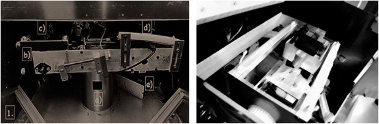
FIGURE 3. Centrifugal Adhesion Balance (1) Side view of CAB–(A) Motor and centrifugal rotating arm, (B) Chamber, (C) Goniometer, (D) Remote tablet and a counterbalance, (E) Control unit or Controller. (2) View of CAB chamber with Goniometer–Camera, light source and sample holder clamps with dome enclosed (Yadav et al., 2018; Young, 1805; Tadmor, 2021; Tadmor, 2013; Tadmor, 2011; Tadmor, 2004; Tadmor et al., 2009; N’guessan et al., 2012; Wasnik et al., 2015; Tadmor et al., 2008; Yadav et al., 2008).

Figure 4 indicates the vectorial representation of forces that are acting on the droplet when it is in the CAB’s chamber (Tadmor, 2004; Tadmor, 2011; Tadmor, 2013). Traditionally with tilting stage method, the method for incline that a drop is subject to is determined by both the varying normal and lateral force that is effective to its weight. As mentioned before, with Centrifugal Adhesion Balance, this issue is resolved when liquid drop of mass m is subject to varying lateral force, that is subject to angular velocity ω respect to radius of rotation, R. In real time, the drop is subject to normal effective to it weight, which is based on the angular tilt, α, that the chamber and drop is subject to and with inclusion of gravitational constant, g. This continuous real time manipulation of the angular velocities and angular tilt causes the chamber and drop to experience a constant normal force condition with varying lateral force or vice versa. This is done in a manner, such that both these forces are decoupled and manipulated to keep one constant force condition while the other force varies.

FIGURE 4

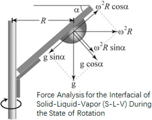
FIGURE 4. Schematic diagram of the forces acting
on a drop in CAB’s chamber (where m is the mass
of drop, $\omega$ is the angular velocity of CAB; $R$ is the
distance between the center of the rotating arm to the
center of mass of the drop; $\alpha$ is the tilt angle of the
CAB’s chamber with respect to horizontal axis;
$g$ is the gravitational acceleration;
$f_{\parallel }$ is lateral force; $f_{\perp }$ is
normal force, with any combination of the
gravitational force and the centrifugal force that help
in manipulating the normal force and lateral force which
is calculated by using the following equations;
$f_{\parallel }=m\left({\omega }^{2}R\cos \alpha -g\sin \alpha \right),$
f⊥=mω2R⁡sin⁡α+g⁡cos⁡α
(Tadmor, 2004; Tadmor, 2021) based on the
force balance analysis.) (Yadav et al., 2018;
Young, 1805; Tadmor, 2021; Tadmor, 2013;
Tadmor, 2011; Tadmor, 2004;
Tadmor et al., 2009;
N’guessan et al., 2012; Wasnik et al., 2015;
Tadmor et al., 2008; Yadav et al., 2008)

CAB is controlled by the software written in MATLAB from the remote desktop through which the control unit receives the signal and manipulates the rotation and the tilt of the chamber. Using this we can obtain any combination of the gravitational force and the centrifugal force that help in manipulating the normal force and lateral force which is calculated by using the following Equation 3 and Equation 4 (Tadmor, 2011; Tadmor, 2004; Tadmor et al., 2009; N’guessan et al., 2012).

$f_{\parallel }=m\left({\omega }^{2}R\cos \alpha -g\sin \alpha \right)(3)$

$f_{\perp }=m\left({\omega }^{2}R\sin \alpha +g\cos \alpha \right)(4)$

where $f_{\parallel }$ is lateral force, $f_{\perp }$ is normal force, m is the mass of drop, $\omega$ is the angular velocity of CAB, $R$ is the distance between the center of the rotating arm to the center of mass of the drop, $\alpha$ is the tilt angle of the CAB’s chamber with respect to horizontal axis and $g$ is the gravitational acceleration.

There are two sets of experiments performed using the CAB with the liquid drop resting on the substrate. In the first one, the drop experiences constant normal force equals to its weight and an increasing lateral force. This increasing lateral force causes the drop to experience force outwards, and so the drop elongates in the direction of force and suddenly slides of the surface as it overcomes the retention force. In the other experiment, the drop experiences a zero lateral force and an increasing normal force. As the normal force increases, the drop elongates away from the surface and one can observe shrinkage of the drop circumference followed by the drop’s detachment or ‘flying’ from the surface.

1) CAB is connected to the power source and the remote desktop placed nearby the CAB.

2) To monitor and for real time observation of the liquid drop placed on the substrate (any given solid surface), AVT Pike CCD camera is used which is directly connected to the portable computer with the CAB analyzer software.

3) The CAB chamber is leveled horizontally using the CAB’s software automated function. And the goniometer is adjusted manually such that the sample holder is levelled horizontally along with the CAB’s chamber.

4) After levelling the chamber, the substrate (given surface) is placed in the sample holder in between the clamps.

5) The tilt of the chamber (CAB plate) is set according to the requirement for the experiment.

6) The drop of required volume is drawn and placed on the substrate using the syringe.

7) Once the drop is placed onto the substrate (given surface), hemispherical glass optical dome is used to cover the sample.

8) Optical dome is used as a sealing agent which helps in suppressing the evaporation of the volatile liquids and to resist any wind effects during the rotation of CAB’s chamber. Sometimes along with the optical dome small water droplets are placed inside near the liquid droplet to maintain the humidity and for suppressing the evaporation effect (Wasnik et al., 2015).

9) Then the MATLAB software is used to run the CAB by setting the constant angular acceleration and the required function according to the type of experiment.

10) The tilt of the CAB’s plate is set according to the function set for the experiment, for sessile drop $\alpha$ = 0°, and for pendant drop $\alpha$ = 180°.

11) The remote desktop is used to record the rpm of the CAB and the portable computer is used to record the images during the experiment.

3 Experiment procedures

3.1 Material preparation (materials and rust formation)

3.1.1 Choice of material

Through literature review we choose to use Galvanized Carbon Steel which is commonly used in industries.

3.1.2 Choice of sample size

For the initial study we choose to cut 1 × 1 × 0.035-inch sheet strips. And for further study, we used 1 × 1 × 0.071-inch sheet strips. The desired stripes from both the sheets were cut with the help of Mechanical Bandsaw which can be seen from Figure 5.

FIGURE 5

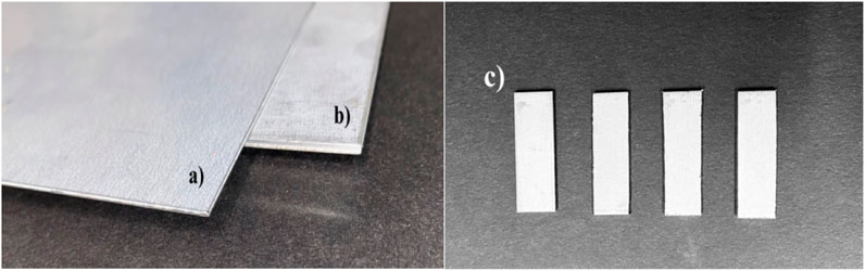
FIGURE 5. Galvanized Carbon Steel sheets (A) 1 × 1 × 0.035-inch sheet (B) 1 × 1 × 0.071-inch sheet (C) the sample strips cut-outs from the sheet (A) and (B) using mechanical bandsaw which are later used in our experiment.

3.1.3 Choice of treatment

We expose the metal strips of thickness 0.035 inch and 0.071 inch to 1M HCl solution for 46 h and 69 h–By placing a small (0.7 mL) drop of 1M HCl solution between the lower part of the metal strip and the supporting plastic petri dish as shown in Figure 6.

FIGURE 6

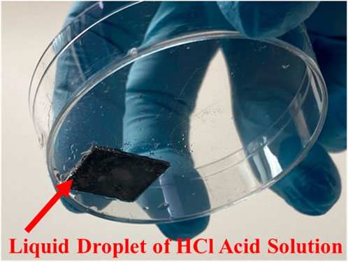
FIGURE 6. A Paintable Galvannealed Low-Carbon Steel strip with a drop of 0.7 mL 1M HCl between its lower surface and the floor of a plastic petri dish that is exposed for 46 h.

3.1.4 Choice of a cleaning procedure

To ensure our results are consistent and represent the chemical changes in the material, we clean the surface from debris. The cleaning was done in the following manner. All samples’ top layer was thoroughly wiped clean six times with a lint-free lab wipe soaked with acetone. In this way, we consider the nature of the metal and not any coating that may have accumulated on it.

3.2 CAB measurement procedures

After cleaning the surface, we placed it in the CAB’s chamber between the holding clamps with acid treated side facing down. The water droplet is thus placed on the cleaned, non-treated side. In such a way, we tested the resilience of the rusted surface to react with the given liquid (i.e., distilled water in our case).

Once the surface is placed in-between the sample holder, we use light air blower to blow the air and to make sure that the surface and the equipment is dust free and has no debris left onto the surface which may affect the experimental results. In order to maintain the humidity and to reduce the effect of evaporation, small water droplets (called as satellite droplets) were placed on the clamps around it. As, if the main drop of water evaporates then the relative humidity will rise to 96% within very few minutes (Wasnik et al., 2015). Then 5 μL distilled water is drawn using the syringe and is placed onto the surface carefully. The sample holder is covered with the hemispherical optical dome and the centrifugal arm (CAB’s chamber) is allowed to rotate at constant acceleration of 3 rpm/s with the function set to maintain the constant zero normal force. Due to which the tilt of the CAB’s chamber will be adjusted automatically to maintain constant zero normal force. The motion of the drop during the experiment is monitored on the remote desktop and all the images taken at approximately 15 frames per second are saved into the specific folder that is created before the start of the experiment which are later used for the analysis and calculation.

The bottom layer of the metal strips like the one that’s shown in Figure 4C with thickness 0.035-inch and 0.071-inch were exposed to 1M HCl solution for a specific time period. For our experiments the exposure time was approximated to be 46 h and 69 h for both the metal strips. The 0.7 mL of 1M HCl solution is drawn by pipet and then a drop of it is placed into a plastic petri dish. The metal strip is then placed onto the drop of acid carefully such that the top layer does not come in contact with the acid drop and only its bottom surface is in contact with the acid drop. The petri dish is placed into the enclosed fume hood and are kept open to avoid any condensation that may occur due to the vapor of HCl solution which may affect the top layer of the strip if the dish is covered with lid. One of the metal strips is taken out after 46 h and other is taken out after 69 h, then the bottom layer of the metal strips is allowed to dry from the acid and the top layer which is not exposed to any acidic solution were cleaned with the lint free cloth soaked in acetone. After we clean it, the sample plate is placed inside the CAB chamber on sample holder and is clamped. As mentioned in the experimental procedure, we run an experiment where a 5 μL distilled water is drawn using the syringe and is placed onto the surface carefully. We posit that the effective change in motion and the change in the contour of the drop (which is the change in the advancing and receding contact angles) in real time as the drop is sliding across the surface, will change with the nature of the surface that is used. As mentioned before, rust corrosion is a voltaic phenomenon, where the bottom layer rust would be able to affect the top layer’s interaction with the liquid, which would mean a change in the Interfacial Modulus (G_S).

For our study, to calculate the interfacial modulus (Gs), the normal force is to be kept constant (zero) and that is done by varying the lateral force and the angle of tilt of the chamber. The experiments start at $\alpha$ = 90 and as the lateral force increases along with the angular acceleration, the tilt of the chamber plate will change such that the effective zero normal force will remain constant and allows the drop to slide in lateral direction rather than detaching it from the surface in the normal direction.

The images which are recorded in the remote desktop during the experiment are analyzed with the CAB analyzer software to get many useful information from each individual image of the drop at particular time. The information we get by processing each image will be as listed and shown in the image below which can be seen from Figure 7:

1) Advancing Contact angle (Left contact angle) (${\theta }_A$)

2) Receding Contact angle (Right contact angle) (${\theta }_R$)

3) Volume of the drop

4) Height of the drop

FIGURE 7

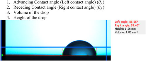
FIGURE 7. Image taken from the CAB Analyzer after processing it. Red lines tangential to the drop outer edges is Left angle (Advancing Contact angle, or Left contact angle ${\theta }_A$) and the Right angle (Receding Contact angle, or Right contact angle ${\theta }_R$). The other drop measurements will include the Height of liquid droplet and the Volume of liquid droplet.

The values of the Advancing Contact angle or Left contact angle ${\theta }_A$, the Receding Contact angle or Right contact angle ${\theta }_R$ , the Height of liquid droplet, and the Volume of liquid droplet will be used to calculate the Interfacial Modulus (Gs).

The values that we get by processing the image will then be used in Eq. 3 to get the lateral force value which we are using for our study to calculate the interfacial modulus (G_S). Equation. 2 is used to calculate the G_S value.

5 Results and discussion

Once we process the experimental results and do calculation based on the obtained value of quantities from CAB analyzer, we get the following values for interfacial modulus with respect to the surface used and the duration of exposure to acid corrosion. For reference, below is an image strip where the drop slides across a carbon steel plate, whose bottom layer has been exposed to acid, for 46 h.

The sequence of images shown in the above figure represents that the drop resting on the surface is experiencing the increasing lateral (centrifugal) force from a) to e), i.e., the lateral force in a) is the least whereas the lateral force in e) is the highest. At the start of experiment the contour of the drop seems to be like in a) with the minimal lateral force, as the lateral force increases the contour of the drop changes and the drop elongates (advancing edge of drop moves) in the direction of lateral force but the receding edge still remains at the same position, now as shown in Figure 8C as the lateral force increases the receding edge also starts to move in the direction of lateral force, which we call it as an onset on motion of the drop (as now the drop is moving as whole). As the lateral force keeps on increasing the drop while finally slide off the surface as shown in Figure 8D and Figure 8E.

FIGURE 8

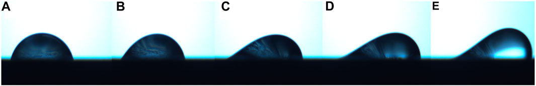
FIGURE 8. Image strip for the water drop on top surface of a rusted metal plate which is experiencing the increasing lateral (centrifugal) force from left to right.

Below are the experiment and calculation results for Interfacial Modulus (G_S) of carbon steel plates, whose bottom layer has been exposed to acid corrosion for different durations.

Following the cleaning procedure, the samples were placed in the CAB chamber and measured for their interfacial modulus. For the table above, we choose the Gs value that corresponds to the first time the receding edge of the drop moved 0.2 mm from the position it is initially rested on. This is marked by the dashed lines in Figure 9, with panels with panels: a) Not treated with acid, b) Treated with 1M HCl for 46 h, c) Treated with 1M HCl for 69 h.

FIGURE 9

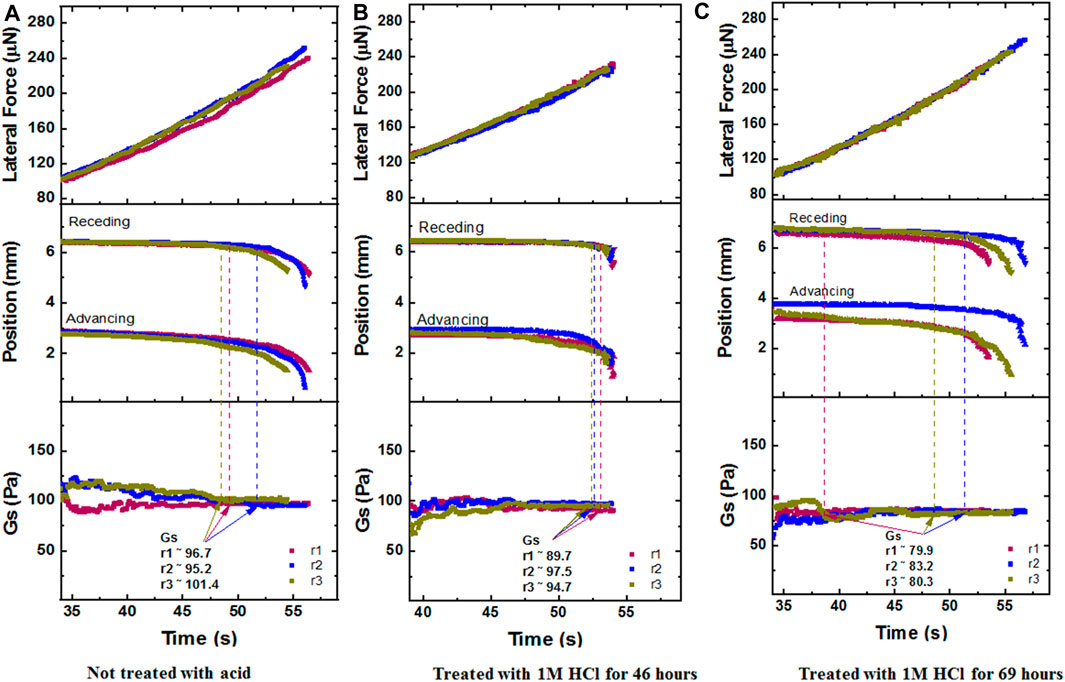
FIGURE 9. CAB Experimental runs Lateral Force, Position, Gs values that correspond to a 5 µL DI water drop sliding on the fresh metal strip (Paintable Galvannealed Low-Carbon Steel Sheet of thickness 0.035 inch), at 0g, with panels: (A) Not treated with acid, (B) Treated with 1M HCl for 46 h, (C) Treated with 1M HCl for 69 h. Here, r1, r2, r3 mean Run 1, Run 2, Run 3.

Following the cleaning procedure, the samples were placed in the CAB chamber and measured for their interfacial modulus. For the table above (Table 1), we choose the Gs value that corresponds to the first time the receding edge of the drop moved 0.2 mm from the position it is initially rested on. This is marked by the dashed lines in Figure 10, with panels a, b, c.

TABLE 1

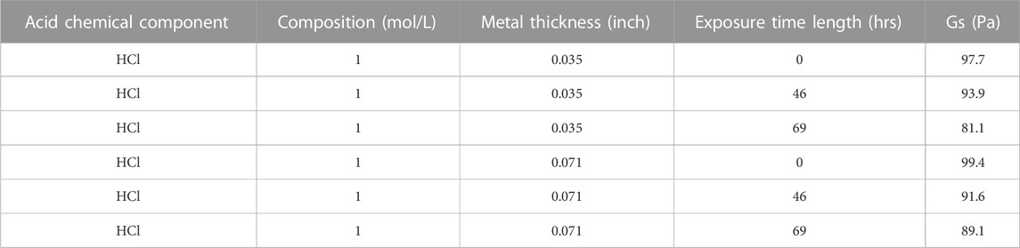
TABLE 1. Summary table of dependent variable of average Interfacial Modulus (Gs) values with respective to independent variables of Substrate Material Type, Sheet Strip Thickness of Galvanized Carbon Steel, Acidic Chemical Material, Acid Composition, Exposure Time for the metal strips at 0 g whose opposite side was treated.

FIGURE 10

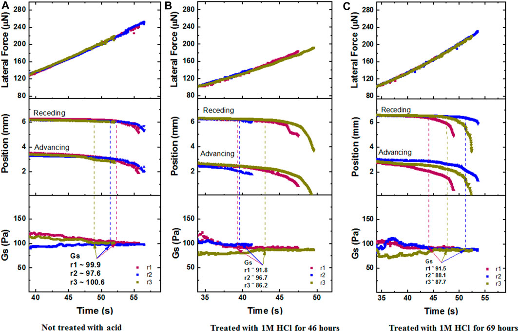
FIGURE 10. CAB Experimental runs Lateral Force, Position, Gs values that correspond to a 5 µL DI water drop sliding on the fresh metal strip (Paintable Galvannealed Low-Carbon Steel Sheet of thickness 0.071 inch), at 0g, with panels: (A) Not treated with acid, (B) Treated with 1M HCl for 46 h, (C) Treated with 1M HCl for 69 h. Here, r1, r2, r3 mean Run 1, Run 2, Run 3.

The results of the experiments have been given in Table 1. The response surface of average Interfacial Modulus (Gs) values with respective to Sheet Strip Thickness of Galvanized Carbon Steel, Exposure Time has been plotted in Figure 11.

FIGURE 11

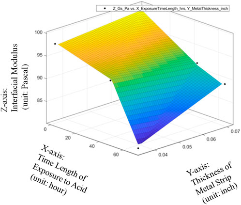
FIGURE 11. Response surface of average Interfacial Modulus (Gs) values with respective to Sheet Strip Thickness of Galvanized Carbon Steel and Exposure Time.

On one hand, it can be seen from Figure 11 that the impact of the metal strip thickness (inch) on the Interfacial Modulus (Gs) is very little if the sheet strip of galvanized carbon steel has not been exposed to the acidic solution. With the increase of galvanized carbon steel’s exposure time in the acidic solution environment, the effect of the Sheet Strip Thickness of Galvanized Carbon Steel on the average Interfacial Modulus (Gs) values will be gradually enhanced. When the exposure time has been larger than 35 h, the Interfacial Modulus (Gs) values will be largely reduced with the decrease of the Sheet Strip Thickness of Galvanized Carbon Steel. Therefore, the whole SURF figure is piecewise with multiple subspaces which can be described with a specific linear function for each subspace.

On the other hand, it can be seen from Figure 11 that the Interfacial Modulus (Gs) will always decrease with longer period of the metal strip of galvanized carbon steel exposed to the acidic solution. Moreover, the gradient or reduction rate of the Interfacial Modulus (Gs) with respective to the exposure time is very small if the Sheet Strip Thickness of Galvanized Carbon Steel is very large while the gradient or reduction rate of the Interfacial Modulus (Gs) with respective to the exposure time is very large if the Sheet Strip Thickness of Galvanized Carbon Steel is very small. Therefore, the pipeline with lower pipeline thickness will have larger change in the Interfacial Modulus (Gs) with respective to the exposure time in the acidic environment and the pipeline with larger pipeline thickness will have smaller change in the Interfacial Modulus (Gs) with respective to the exposure time in the acidic environment.

The above observations can be further from the contour plot of Figure 12.

FIGURE 12

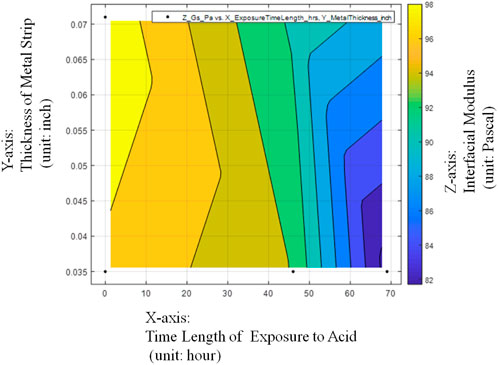
FIGURE 12. Contour plot of average Interfacial Modulus (Gs) values with respective to Sheet Strip Thickness of Galvanized Carbon Steel and Exposure Time.

If the linear function of average Interfacial Modulus (Gs) with multiple independent variables (Sheet Strip Thickness of Galvanized Carbon Steel, MT with the unit of inch and Exposure Time with the unit of time, ET) is to be expected, the quantitative expression should be given as below:

$G_s=95.6-0.1851\times ET+68.52\times MT(5)$

The metrics of data fitting are SSE: 39.86, R-square: 0.8173, Adjusted R-square: 0.6955, RMSE: 3.645. It can be seen from Figure 13 that the performance of data fitting is not good enough with the R-square value of only 0.8173 since the standards for a good R-Squared reading would be generally be seen as showing a high level of correlation if R-squared value is 0.9 or above.

FIGURE 13

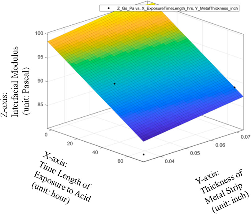
FIGURE 13. Linear data fitting of average Interfacial Modulus (Gs) with respective to Sheet Strip Thickness of Galvanized Carbon Steel and Exposure Time, with metrics of data fitting.

If the cross-product embedded quadratic function of average Interfacial Modulus (Gs) with multiple independent variables (Sheet Strip Thickness of Galvanized Carbon Steel, MT with the unit of inch and Exposure Time, ET with the unit of time to be hour) is to be expected, the quantitative expression should be given as below:

$G_s=98.63-0.08533\times ET-1.587\times MT-0.002993\times {ET}^2+1.829\times ET\times MT(6)$

The metrics of data fitting are SSE: 21.61, R-square: 0.9009, Adjusted R-square: 0.5046, RMSE: 4.649. It can be seen from Figure 13 that the performance of data fitting is better than the linear data fitting since the R-square value of 0.9009 can satisfy the general standards for a good R-Squared reading with a high level of correlation to be 0.9 or above.

Linear model Poly11:

$G_s=P_{00}+P_{10}\times ET+P_{01}\times MT(7)$

Coefficients (with 95% confidence bounds):$P_{00}$ = 95.6 (79.57, 111.6)$P_{10}$ = −0.1851 (−0.3502, −0.02001)$P_{01}$ = 68.52 (−194.6, 331.6)

Goodness of fit:SSE: 39.86R-square: 0.8173Adjusted R-square: 0.6955RMSE: 3.645

Linear model Poly21:

$G_s=P_{00}+P_{10}\times ET+P_{01}\times MT+P_{20}\times {ET}^2+P_{11}\times ET\times MT(8)$

Coefficients (with 95% confidence bounds):$P_{00}$ = 98.63 (−27.02, 224.3)$P_{10}$ = −0.08533 (−4.245, 4.074)$P_{01}$ = −1.587 (−2238, 2235)$P_{20}$ = −0.002993 (−0.05223, 0.04625)$P_{11}$ = 1.829 (−44.88, 48.53)

Goodness of fit:SSE: 21.61R-square: 0.9009Adjusted R-square: 0.5046RMSE: 4.649

General model:

$G_s=P_{00}+P_{20}\times {ET}^2+P_{02}\times {MT}^2(9)$

Coefficients (with 95% confidence bounds):$P_{00}$ = 96.59 (87.8, 105.4)$P_{20}$ = −0.002828 (−0.004829, −0.0008264)$P_{02}$ = 646.4 (−1397, 2689)

Goodness of fit:SSE: 27.01R-square: 0.8762Adjusted R-square: 0.7937RMSE: 3

General model:

$G_s=P_{00}+P_{20}\times {ET}^2+P_{02}\times {MT}^2+P_{10}\times ET(10)$

Coefficients (with 95% confidence bounds):$P_{00}$ = 96.52 (81.13, 111.9)$P_{20}$ = −0.002993 (−0.01616, 0.01018)$P_{02}$ = 646.4 (−2734, 4027)$P_{10}$ = 0.01159 (−0.8825, 0.9057)

Goodness of fit:SSE: 26.96R-square: 0.8764Adjusted R-square: 0.691RMSE: 3.672

Therefore, it can be seen from Figures 14–16 that only the quadratic function with cross product term will give the performance to satisfy the general standards for a good R-Squared reading with a high level of correlation to be 0.9 or above even though it will add the difficulty to the global optimization in the future. Thanks to the cross-product term, the quadratic function of Gs = 98.63–0.08533*ET-1.587*MT-0.002993*ET^2 + 1.829*ET*MT can provide the good data fitting for the preliminary quantitative relationship among average Interfacial Modulus (Gs), Sheet Strip Thickness of Galvanized Carbon Steel (MT) and Exposure Time (ET). Based on this, it can be verified that with different durations of acid corrosion that the bottom layer of the carbon steel plate is subject to, there is change in the value of Interfacial Modulus (G_S). With increasing duration of acid corrosion, the top layer’s interaction with the liquid drop sliding across the surface changes in such a manner, that the G_S value decreases exponentially with linear increase in time duration that the bottom layer of plate is place in the acid. This proves the basic hypothesis, that rust corrosion inside the pipeline can be considered a voltaic phenomenon such that bottom layer’s corrosion will affect the top layer of metal plate. Despite the non-existent observational change in rust detection at the top layer, the change in rust formation of bottom layer will change the topographical nature of top layer of the metal, which would cause a value change in G_S.

FIGURE 14

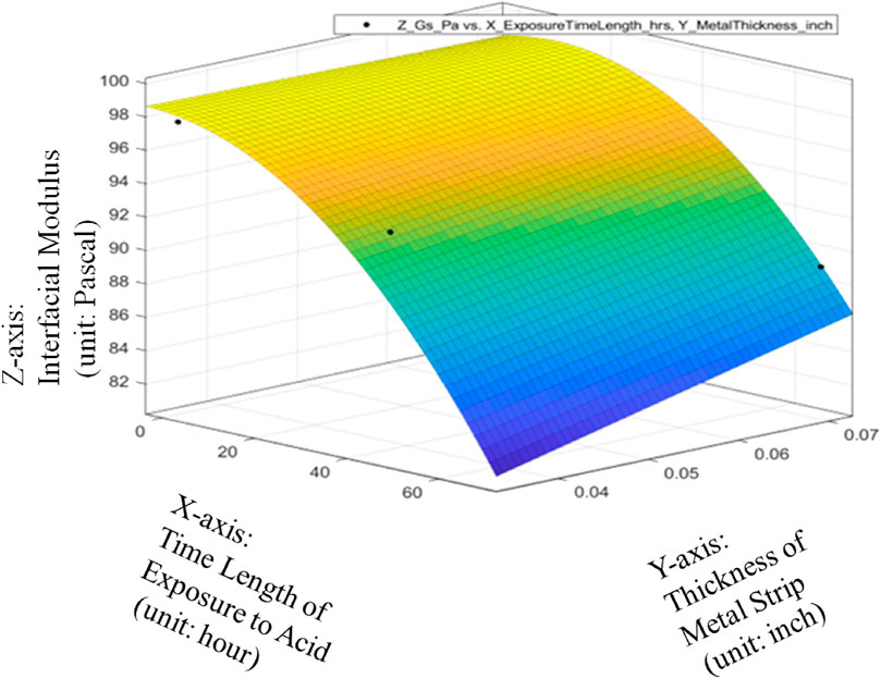
FIGURE 14. Quadratic data fitting of average Interfacial Modulus (Gs) with respective to Sheet Strip Thickness of Galvanized Carbon Steel and Exposure Time, with metrics of data fitting.

FIGURE 15

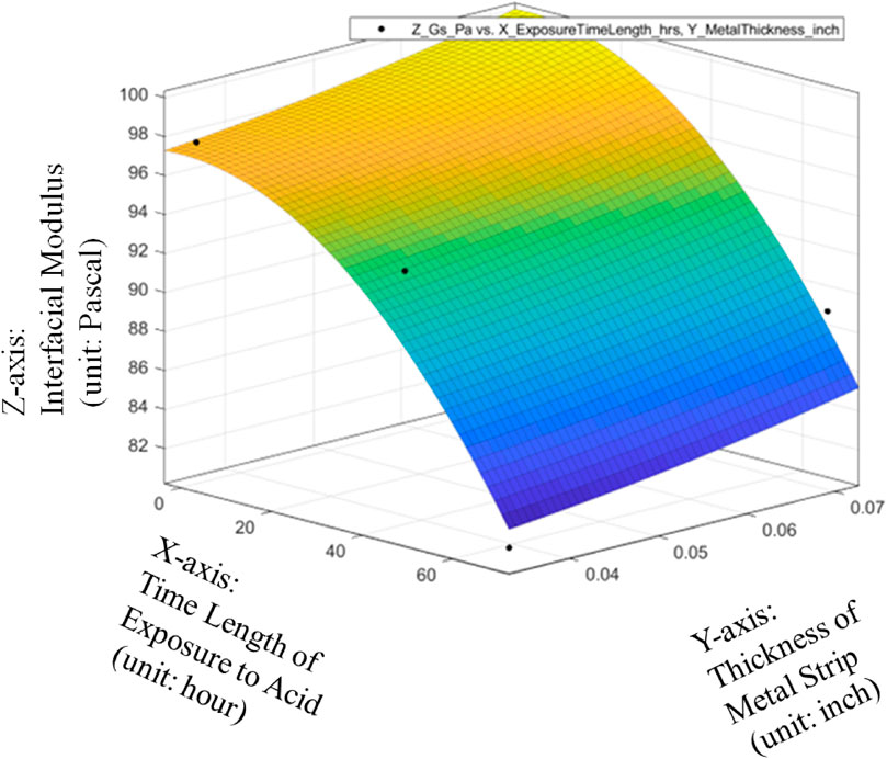
FIGURE 15. Quadratic data fitting of average Interfacial Modulus (Gs) with respective to Sheet Strip Thickness of Galvanized Carbon Steel and Exposure Time, with metrics of data fitting.

FIGURE 16

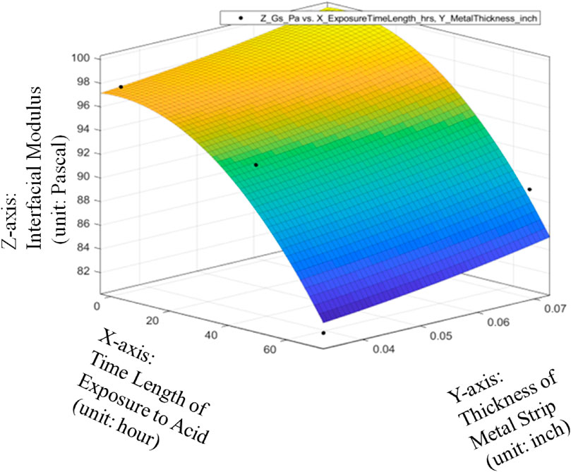
FIGURE 16. Quadratic data fitting of average Interfacial Modulus (Gs) with respective to Sheet Strip Thickness of Galvanized Carbon Steel and Exposure Time, with metrics of data fitting.

As Interfacial modulus can be summarized in terms of solid layer’s resilience to interact with the liquid, which is based on interfacial molecules within solid’s first monolayer, the value change for these experiments means that solid top layer is affected by rust at the bottom layer of the metal. The Gs value is characteristically dependent on many factors such as lateral force and drop’s contour, which is best summarized in the contact angles at the drop’s edge throughout each run. The contact angle plots for each scenario for the carbon steel used, are presented in the appendix section. Thereby as observed in our experiments, the decrease in the Gs value means greater interaction, thereby greater adhesion of the liquid across the top layer, which means increase in corrosion duration stipulates the drop is being retained longer when sliding across the surface.

With different durations of acid corrosion that the bottom layer of the carbon steel plate is subject to, there is change in the value of Interfacial Modulus (G_S). With increasing duration of acid corrosion, the top layer’s interaction with the liquid drop sliding across the surface changes in such a manner, that the G_S value decreases exponentially with linear increase in time duration that the bottom layer of plate is place in the acid. This proves the basic hypothesis, that rust corrosion inside the pipeline can be considered a voltaic phenomenon such that bottom layer’s corrosion will affect the top layer of metal plate. Despite the non-existent observational change in rust detection at the top layer, the change in rust formation of bottom layer will change the nature of top layer of the metal, which would cause a value change in G_S. As Interfacial modulus can be summarized in terms of solid layer’s resilience to interact with the liquid, which is based on interfacial molecules within solid’s first monolayer, the value change for these experiments means that solid top layer is affected by rust at the bottom layer of the metal. In our experiments, the decrease in value means greater interaction, thereby greater adhesion of the liquid across the top layer, which means increase in corrosion duration stipulates the drop is being retained longer when sliding across the surface.

6 Conclusion

The results from the experiment prove one pertinent issue to the oil and gas industry has been answered, can rust be detected through a non-invasive method? From our results, it seems so to be the case. We theorized that rust formation is a voltaic phenomenon, where the electronegativity of the metal when exposed to acid corrosion would change the interfacial properties of both layers of metal, with only one layer being exposed to acid corrosion. In our results, Gs is decreasing with respect to the duration that the bottom layer is exposed to the acid, meaning the interfacial interaction is affected in such a manner, that the molecular attraction between the top solid layer and liquid increases. This would cause greater adhesion and greater retention force which is verily summarized in the Interfacial Modulus property. The reasons for this, again, can denoted to the intermolecular attraction being affected by the electronegativity caused in the bottom layer that is exposed to rust. The next issue would lie on how to create an industrial application of this equipment and research. One possible solution is to set stations across different points at the facility where corrosion is best detected or use places where corrosion is already being detected. Another field inspection by any personnel at site to detect rust by observing motion of various micro-droplets across the surface of pipeline. Various ideas can be formulated to bring the scientific research into industrial reality, but it is certain that this research has allowed us to further explore towards the right path in the field of rust corrosion and detection.

Data availability statement

The original contributions presented in the study are included in the article/Supplementary Material, further inquiries can be directed to the corresponding author.

Author contributions

All authors listed have made a substantial, direct, and intellectual contribution to the work and approved it for publication.

Funding

The research was supported by the Center for Midstream Management and Science at Lamar University.

Conflict of interest

The authors declare that the research was conducted in the absence of any commercial or financial relationships that could be construed as a potential conflict of interest.

Publisher’s note

All claims expressed in this article are solely those of the authors and do not necessarily represent those of their affiliated organizations, or those of the publisher, the editors and the reviewers. Any product that may be evaluated in this article, or claim that may be made by its manufacturer, is not guaranteed or endorsed by the publisher.

Supplementary material

The Supplementary Material for this article can be found online at: https://www.frontiersin.org/articles/10.3389/fceng.2023.1150776/full#supplementary-material

References

Butt, H. J., Berger, R., Steffen, W., Vollmer, D., and Weber, S. A. (2018). Adaptive wetting—Adaptation in wetting. Langmuir 34 (38), 11292–11304. doi:10.1021/acs.langmuir.8b01783

PubMed Abstract | CrossRef Full Text | Google Scholar

Carré, A., Gastel, J. C., and Shanahan, M. E. (1996). Viscoelastic effects in the spreading of liquids. Nature 379 (6564), 432–434. doi:10.1038/379432a0

CrossRef Full Text | Google Scholar

Dupré, A., and Dupré, P. (1869). Théorie mécanique de la chaleur. Gauthier-Villars.

Google Scholar

Koch, G. H., Brongers, M. P., Thompson, N. G., Virmani, Y. P., and Payer, J. H. (2002). Corrosion cost and preventive strategies in the United States (No. FHWA-RD-01-156, R315-01). United States: Federal Highway Administration.

Google Scholar

Lester, G. R. (1961). Contact angles of liquids at deformable solid surfaces. J. Colloid Sci. 16 (4), 315–326. doi:10.1016/0095-8522(61)90032-0

CrossRef Full Text | Google Scholar

Meiron, T. S., Marmur, A., and Saguy, I. S. (2004). Contact angle measurement on rough surfaces. J. colloid interface Sci. 274 (2), 637–644. doi:10.1016/j.jcis.2004.02.036

PubMed Abstract | CrossRef Full Text | Google Scholar

N’guessan, H. E., Leh, A., Cox, P., Bahadur, P., Tadmor, R., Patra, P., et al. (2012). Water tribology on graphene. Nat. Commun. 3 (1), 1242. doi:10.1038/ncomms2247

PubMed Abstract | CrossRef Full Text | Google Scholar

Pethica, B. A. (1977). The contact angle equilibrium. J. Colloid Interface Sci. 62 (3), 567–569. doi:10.1016/0021-9797(77)90110-2

CrossRef Full Text | Google Scholar

Rusanov, A. I. (1975). Theory of wetting of elastically deformed bodies. 1. Deformation with a finite contact-angle. Colloid J. USSR 37 (4), 614–622.

Google Scholar

Shanahan, M. E. R., and Degennes, P. G. (1986). The ridge produced by a liquid near the triple line solid liquid fluid. Comptes Rendus De. L Acad. Des. Sci. Ser. Ii 302 (8), 517–521.

Google Scholar

Shanahan, M. E. R., and de Gennes, P. G. (1987). “Equilibrium of the triple line solid/liquid/fluid of a sessile drop,” in Adhesion 11. Editor K. W. Allen (Dordrecht: Springer). doi:10.1007/978-94-009-3433-7_5

CrossRef Full Text | Google Scholar

Tadmor, R., Chaurasia, K., Yadav, P. S., Leh, A., Bahadur, P., Dang, L., et al. (2008). Drop retention force as a function of resting time. Langmuir 24 (17), 9370–9374. doi:10.1021/la7040696

PubMed Abstract | CrossRef Full Text | Google Scholar

Tadmor, R., Bahadur, P., Leh, A., N’guessan, H. E., Jaini, R., and Dang, L. (2009). Measurement of lateral adhesion forces at the interface between a liquid drop and a substrate. Phys. Rev. Lett. 103 (26), 266101. doi:10.1103/physrevlett.103.266101

PubMed Abstract | CrossRef Full Text | Google Scholar

Tadmor, R. (2004). Line energy and the relation between advancing, receding, and young contact angles. Langmuir 20 (18), 7659–7664. doi:10.1021/la049410h

PubMed Abstract | CrossRef Full Text | Google Scholar

Tadmor, R. (2011). Approaches in wetting phenomena. Soft Matter 7 (5), 1577–1580. doi:10.1039/c0sm00775g

CrossRef Full Text | Google Scholar

Tadmor, R. (2013). Misconceptions in wetting phenomena. Langmuir 29 (49), 15474–15475. doi:10.1021/la403578q

PubMed Abstract | CrossRef Full Text | Google Scholar

Tadmor, R. (2021). Open problems in wetting phenomena: Pinning retention forces. Langmuir 37 (21), 6357–6372. doi:10.1021/acs.langmuir.0c02768

PubMed Abstract | CrossRef Full Text | Google Scholar

Wasnik, P. S., N’guessan, H. E., and Tadmor, R. (2015). Controlling arbitrary humidity without convection. J. colloid interface Sci. 455, 212–219. doi:10.1016/j.jcis.2015.04.072

PubMed Abstract | CrossRef Full Text | Google Scholar

Yadav, P. S., Bahadur, P., Tadmor, R., Chaurasia, K., and Leh, A. (2008). Drop retention force as a function of drop size. Langmuir 24 (7), 3181–3184. doi:10.1021/la702473y

PubMed Abstract | CrossRef Full Text | Google Scholar

Yadav, P. S., Gulec, S., Jena, A., Tang, S., Yadav, S., Katoshevski, D., et al. (2018). Interfacial modulus and surfactant coated surfaces. Surf. Topogr. Metrology Prop. 6 (4), 045007. doi:10.1088/2051-672x/aae808

CrossRef Full Text | Google Scholar

Young, T. (1805). III. An essay on the cohesion of fluids. Philosophical Trans. R. Soc. Lond. 95, 65–87.

Google Scholar