Numerical Analysis of Flow Characteristics of Upper Swirling Liquid Film Based on the Eulerian Wall Film Model

The Upper Swirling Liquid Film (USLF) phenomenon that occurs in the upper cylinder of the Gas–Liquid Cylindrical Cyclone (GLCC) separator is the direct cause of the low separation efficiency of the liquid phase. In this study, first, the USLF formation and development were simulated by an improved Eulerian-EWF coupled simulated method. By introducing a profile-defined inlet boundary and considering entrainment droplet size distributions, the Eulerian-EWF method got reasonable results which agreed well with the experimental. Then, the flow characteristics and changing laws of the USLF including film thickness, film axial velocity, and film tangential velocity were analyzed by this method under different gas–liquid flow rates. It suggested that the liquid film thickness often reaches a maximum at the aspect ratio (z-z₀)/D=(1.2–3.9) above the tangential inlet, and the film thickness appears to be more sensitive to the gas flow than to the liquid flow. For the film axial velocity, the direction of film velocity on the front and back sides seems to be generally opposite. Finally, typical distributions of the aforementioned USLF variables were presented and corresponded accordingly, and two obvious rules were found. One is that the position where the thickest liquid film is located always corresponds to the position where the axial film velocity turns from positive to negative for the first time. The other is that the tangential film velocity has a strong synchronous relationship with the film thickness. This research might provide somewhat valid information for the future LCO-prevented measurement in GLCC separators.

Introduction

As a new type of gas–liquid separator, Gas–Liquid Cylinder Cyclone (GLCC), has recently drawn a lot of attention in offshore petroleum engineering for its advantages of compact structure, low cost, and high efficiency. A GLCC mainly consists of a vertical pipe containing a downward-inclined tangential inlet and two outlets that are located at the top and bottom to transport the gas and liquid phase respectively, as shown in Figure 1. The tangential feed inlet forces a swirling motion in the multiphase flow and produces a centrifugal force. Meanwhile, gravity causes the liquid to accumulate in the lower part, while the gas gathers in the upper part. Finally, the gas and liquid phase can be separated efficiently.

FIGURE 1

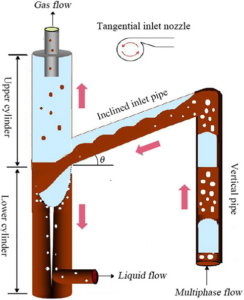
FIGURE 1. Structure and operating principle of a GLCC.

However, the application of GLCC is seriously restricted by common occurrences of the efficiency-harmed Liquid Carry-Over (LCO) phenomenon, which calls for a thorough solution. One of its direct causes is the overflow of Upper Swirling Liquid Film (USLF) in the upper cylinder, which has been proposed by Chirinos (Chirinos et al., 2000) and Hreiz (Hreiz et al., 2014). The USLF is a kind of liquid film that exists in the upper space and swirls continuously around the cylinder wall. It was suggested that the liquid phase separation efficiency of GLCC is very closely related to the USLF flow regimes (Hreiz et al., 2014); (Ti et al., 2019). Their relationship is so tight that how the swirling liquid film behaves and affects the separation efficiency deserves us to pay more attention to in later research.

In fact, the study of USLF is by no means limited to the GLCC separator. This kind of swirling liquid film is universal in any gas–liquid separators or pipes with tangential inlets (Ahmed et al., 2011); (Yang et al., 2015) or helical vanes (Kataoka et al., 2009); (Xiong et al., 2014); (Funahashi et al., 2018). Compared with the ordinary annular flow in a gas–liquid two-phase pipe, the swirling liquid film has two distinct characteristics: 1) The movement of the liquid film includes not only an axial component but also a tangential component; 2) The axial direction of liquid film movement is usually unstable. At present, there have been many studies on the ordinary annular flow. But the reports on the swirling liquid film have not appeared until recent years (Kataoka et al., 2009); (Funahashi et al., 2018); (Liu and Bai, 2015); (Ding et al., 2022). Kataoka (Kataoka et al., 2009) studied the differences between the axial pressure drop and the flow regimes transformation line between a swirling liquid film and an ordinary annular film. Liu (Liu and Bai, 2015) first described the decay of swirling intensity for gas–liquid two-phase flow. Funahashi (Funahashi et al., 2018) calculated the interface friction coefficient for the swirling liquid film by experiments and found that the interface friction coefficient of swirling liquid film is larger than that of the ordinary annular liquid film. It can be seen that these reports generally focused on the flow regimes judgment (Kataoka et al., 2009) or the interfacial friction coefficient (Funahashi et al., 2018), or the axial pressure drop (Kataoka et al., 2009). Relevant literature about the flow characterization of swirling liquid film is still absent, such as the description of film tangential velocity and axial velocity. In addition, the research on swirling liquid film in recent years was mostly carried out in pipes with helical vanes. While the swirling liquid film in pipes with tangential inlets has its particularities due to its asymmetry. In practical engineering, tangential inlets are very common, and the swirling liquid film will easily occur at this moment. Therefore, detailed studies about the swirling liquid film will assist in the mechanism understanding of gas–liquid two-phase flow.

For a three-dimensional swirling liquid film, the experimental method seems low and cost-efficient. But the CFD numerical simulation method provides a good opportunity because it offers ways to achieve the flow parameters of the liquid film. Nevertheless, there are difficulties in the numerical simulation of the liquid film. Generally, the simulation of the liquid film can be divided into the microscopic scale, the macroscopic scale, and the mesoscale. For the microscopic problem (which is closely related to the migration of the gas–liquid interface), scholars often use the Lattice-Boltzmann method (Li et al., 2021) or the Molecular Dynamics method. This kind of method can be merely applied in micro spaces. If it was used for the gas–liquid interface problem of industrial size equipment, extremely high computational memory will be required. For the mesoscale problem (which mainly refers to the liquid film in a local-limited 2D or 3D flow field), the commonly used methods are Level Set + VOF method, the Front Tracking Method (FTM) et al. But this kind of a calculation model still needs large amounts of grids, and it faces difficulties when used in a complex 3D-turbulent flow field. For the macroscopic problem (which mainly includes the liquid film flow pattern, mass, or heat transfer processes in engineering equipment), the aforementioned simulation methods cannot meet its requirements obviously. In 2014, a new-developed method—the Eulerian Wall Film (EWF) model—was specially introduced by ANSYS company to calculate the thin liquid film in 3D spaces (Punekar et al., 2014). Compared with those traditional numerical methods, the EWF model can obtain detailed film flow parameters and calculate more complex flow fields with extremely less grid scale. Scholars have made plenty of attempts to utilize the EWF model and have obtained meaningful liquid film results in many applications (Punekar et al., 2014); (Ying et al., 2016); (Yajun et al., 2019); (Min et al., 2015); (Paz et al., 2017), such as the spray process in an Airblast atomizer (Punekar et al., 2014), film formation in a Venturi flow sensor (Ying et al., 2016) or an axial flow cyclone (Yajun et al., 2019), condensate collection in a stack of power plant (Min et al., 2015) and even human cough process (Paz et al., 2017). They have proved the practicability of the EWF model through its application still calls for wide validation.

Considering the foregoing reasons, a feasible simulated method for the USLF film in GLCC is urgently desired with the assistance of the EWF model. In this article, a film simulation method was successfully developed after comparing two coupling ways between the wall film and the main flow field. As a supplementary, an improved inlet boundary and the Population Balanced Model (PBM) were also introduced. The result of this simulation agrees well with the experiments. Then, the liquid film thickness, film axial velocity, and film tangential velocity of the USLF were analyzed detailed and quantitatively. Based on these results, the changing laws of USLF with the gas and liquid flow rates were studied. Subsequently, the flow characteristics of the liquid film under different USLF flow regimes were discussed respectively. Finally, typical distributions of flow parameters of USLF have summarized accordingly.

Swirling Film in GLCC

The USLF in a GLCC is distinct from other ordinary swirling films. Before the formation of USLF in the GLCC`s main cylinder, the gas–liquid two-phase flow has been pre-separated in the inclined inlet pipe. Thus, the liquid holdup distribution of the feeding flow that is used to form a USLF is not uniform. This makes a huge influence on the USLF development. From previous studies, a stratified flow in the inclined pipe would induce a USLF with a less liquid flow rate, and an annular flow would bring a USLF with a larger liquid flowrate. This process is closely related to the mechanism of the USLF formation.

From our observation, the source of a USLF can be divided into two parts: one is the discrete phase (droplets), and the other is the continuous phase (liquid stream), which has been labeled as ‘①’ and ‘②’ respectively in Figure 2. The former means that there is a short-circuit flow directly streaming into the upper cylinder space from the top wall of the inclined inlet pipe, and the latter source means that those entrained droplets in the gas flow will be collected by the cylinder wall under centrifugal and inertial forces. Therefore, different from other ordinary swirling films, the formation process of USLF cannot be merely equaled to the impacting process of mist flow. For the USLF, an extra streaming process of the short-circuit flow should be investigated as well due to the pre-separation of the inclined inlet pipe.

FIGURE 2

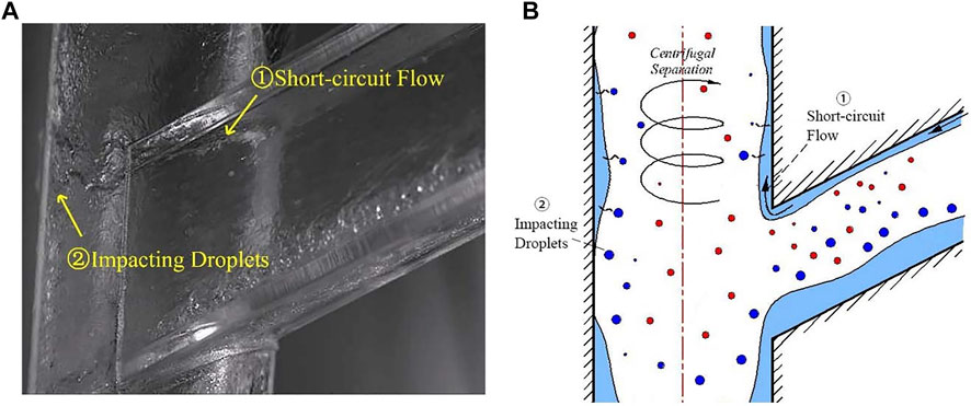
FIGURE 2. Illustration (A) and the schematic diagram (B) of USLF Formation in GLCC: (1) Direct short-circuit flow from the inlet; (2) Droplets impacting due to centrifugal separation.

Methods

In this article, both simulated and experimental methods were adopted to study the USLF phenomenon and provide reliable results.

Simulated Object

The dimensions of simulated GLCC are shown in Figure 3. Its cylinder I.D. was 74 mm (D = 74 mm), and the inclined inlet I.D. was 54 mm, with an inclined angle of −27° and a circle-to-rectangle transition section. The upper cylinder space was defined as the region beginning from the entrance junction located at z₀ = 1310 mm to the gas outlet that is located at z = 2400 mm. Moreover, a liquid stable level should be set among the lower cylinder to avoid excessive gas escaping from the bottom outlet. In the simulation, this level was set as 900 mm, which was similar to our experiments.

FIGURE 3

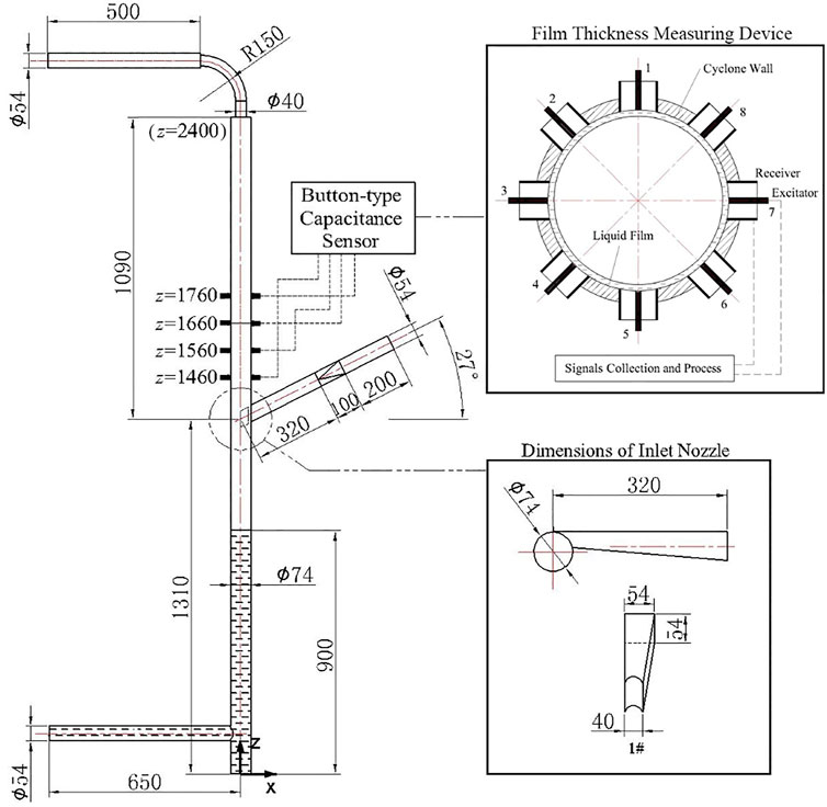
FIGURE 3. Dimensions of the simulated GLCC (the liquid level = 900 mm) and Schematic diagram of button-type capacitance film thickness measuring device.

To verify the simulation method of liquid film, a Button-type Capacitance Sensor was designed to measure the thickness of the liquid film. Four axial positions were measured in the upper cylinder of the tested GLCC, each of which contained eight electrodes that were uniformly distributed along the circumference. Their locations are depicted as Figure 3. This button-type electrode consisted of an exciting electrode (the exciter) and a receiving electrode (the receiver). The voltage difference between the exciter and the receiver reflects the thickness of the liquid film is measured. Remarkably, the prominent advantage of this equipment was its extremely low interference on the measured gas–liquid flow. Because these button-type electrodes were all embodied in the cylinder wall and their inner surface had exactly the same radian as the cylinder pipe wall, which could be seen in Figure 3. This design ensured that the flow of liquid film would not be affected by the sensor. The measurement ability ranged from 0.2 to 5.0 mm, and its accuracy was 0.01 mm.

The fluid properties used in this article were air (the density was 1.225 kg/m³ and the viscosity was 0.000018 Pas) and water (the density was 998.6 kg/m³, the viscosity was 0.001 Pas, and the surface tension was 0.07182N/m). The gas–liquid flowrates simulated in this article included two no-LCO conditions (130m³/h-1.8 m³/h, 160m³/h-0.9 m³/h) and three LCO conditions (160m³/h-1.8 m³/h, 190m³/h-1.8 m³/h, 160m³/h-2.7 m³/h).

EWF Coupling Method

Principle of the EWF Method

In the Eulerian Wall Film (EWF) model, the coupling program of a liquid film with the gas–liquid two-phase flow field is realized by the transition of sources in the mass equation (Eq. 1) and momentum equation (Eq. 2).

$\frac{\partial h}{\partial t}+{\nabla }_s\cdot \left[h{\overrightarrow{V}}_f\right]=\frac{{\dot{m}}_s}{{\rho }_l},(1)$

$\frac{\partial h{\overrightarrow{V}}_f}{\partial t}+{\nabla }_s\cdot \left(h{\overrightarrow{V}}_f{\overrightarrow{V}}_f\right)=-\frac{h{\nabla }_s{P}_L}{{\rho }_l}+\left({\overrightarrow{g}}_{\tau }\right)h+\frac{3}{2{\rho }_l}{\overrightarrow{\tau }}_{fs}-\frac{3v_l}{h}{\overrightarrow{V}}_f+\frac{{\dot{q}}_s}{{\rho }_l},(2)$

where the ρ_l is the secondary phase density, the h is the film thickness, ∇_S is the surface gradient operator, ${\overrightarrow{V}}_f$ is the mean film velocity and the ${\dot{m}}_s$ is the mass source per unit wall area. The P_L includes the effects of gas flow pressure, the gravity component normal to the wall surface, the ${\overrightarrow{\tau }}_{fs}$ is the viscous shear force at the gas-film interface.

When the EWF model is interact with the Eulerian Multiphase model, the film is calculated from the liquid phase volume fraction and the flow conditions. If the liquid phase is captured to form the liquid film, the liquid phase will be removed from the equations of the multiphase flow model. If the film splashes or peels away under a sudden change of wall, the liquid film will return to the liquid phase of the multiphase flow field from the EWF equations. The calculations of the mass source term ${\dot{m}}_s$ and the momentum source term ${\dot{\overrightarrow{q}}}_s$ are listed as follows:

${\dot{m}}_s={\alpha }_l{\rho }_l{V}_{\text{ln}}A,(3)$

${\dot{\overrightarrow{q}}}_s={\dot{m}}_s{\overrightarrow{V}}_l,(4)$

where the α_l is the secondary phase volume fraction, the V_ln is the phase velocity normal to the wall surface, the A is the wall surface area, and the ${\overrightarrow{V}}_l$ is the secondary phase velocity vector.

In this article, the interactions of gravity, wall shear force, pressure gradient force, surface tension, and the diffusive term were all considered. The development of liquid film thickness within 2.5 s were shown in Figure 4. It can be clearly seen that the Eulerian-EWF coupling way can simulate the stable and practical liquid film. The detailed settings of this method will be given in Section 2.2.4.

FIGURE 4

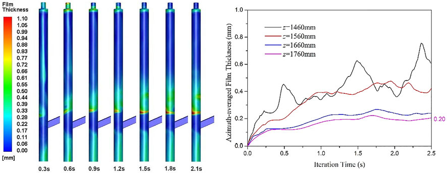
FIGURE 4. Thickness of the developing film by Eulerian-EWF coupling way.

Supplement for the EWF Model——the Continuous Liquid Phase

The pre-separation effect of the inclined inlet directly influences the gas–liquid separation in the main cylinder. A stratified flow can easily appear in the inlet, resulting in an uneven gas–liquid feeding before the cylinder separation. Therefore, in this article, the inlet boundary was improved using a profile-defined method.

First, the gas–liquid flow patterns in the inclined inlet were judged for different operating conditions by the classical flow pattern model. For our experiments, the stratified flow, annular flow, and intermittent flow were observed in the inclined inlet. The Taitel criterion model (Eq. 5) (Taitel and Dukler, 1976) was adopted to judge between the stratified flow and non-stratified flow (including the annular flow and the intermittent flow), and the Barnea criterion model (Eq. 6) (Barnea, 1987) was adopted to judge between the annular flow and the intermittent flow.

$\sqrt{\frac{{\rho }_g}{{\rho }_l-{\rho }_g}}\frac{v_{sg}}{\sqrt{g{D}_{in}\cos \theta }}\left[\frac{1}{{\left(1-{\tilde{h}}_l\right)}^2}\frac{{\tilde{v}}_g^2\sqrt{1-{\left(2{\tilde{h}}_l-1\right)}^2}}{{\tilde{A}}_g}\right]\ge 1,(5)$

$\widetilde{h_l}<0.35,(6)$

where the dimensionless parameter ${\tilde{h}}_l$ means $h_l/D_{in}$, and the ${\tilde{v}}_g$ means $v_g/v_{sg}$. The h_l is the height of the liquid layer in the stratified flow, the D_in is the diameter of the inlet pipe (D_in = 54 mm), and the θ is the inclined angle of the inlet pipe (θ = -27°), and the v_sg is the superficial gas velocity in the inlet pipe.

Then, the flow parameters were calculated for each pattern by the separated fluid method. The gas–liquid profile at the inlet boundary sections can be described and calculated from the momentum equations of the gas and liquid phase, which are too commonly used to be repeated here. Finally, these parameters were programmed to define the gas–liquid profile and docked with the inlet boundary setting by the User Defined Function (UDF) in simulation.

Supplement for the EWF Model——the Droplet Phase

Except for the inlet continuous phase, the influence of droplet size distribution was also important to predict the film formation. In this study, the effects of droplet size distribution were considered by the Population Balanced Model (PBM). This model allows self-defining of the entrainment droplets' size distribution under the Eulerian-Eulerian approach. According to a large number of previous measurement data by aerosol particle size spectrometer, the following formula was recommended here to describe the particle distribution of droplets (Ti, 2019):

$f\left(d\right)=-\frac{2.09}{d}Y\left(d\right)\cdot \ln \left[Y\left(d\right)\right],(7)$

where the d is the diameter size of a certain droplet, and the cumulative oversize distribution of droplet size, Y(d), could be written as the Eq. 8.

$Y\left(d\right)=e^{-{\left(\frac{d}{16.21-0.42v_{sg}}\right)}^{2.09}}.(8)$

Simulated Strategy and Program

The EWF model calls for high stability and accuracy when iterating. Thus, before the EWF calculation, it needs to prepare a high-quality unsteady gas–liquid two-phase flow field. We recommended an iteration time length of (3–6)s for the EWF calculation to get a fully-development film. Other detailed settings during the calculation can be seen totally in Table 1.

TABLE 1

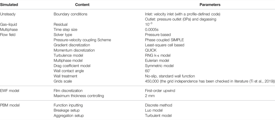
TABLE 1. Settings of the whole simulated program.

Validation of Simulation

Taking the condition of 160 m³/h (gas flowrate) and 1.8 m³/h (liquid flowrate) as examples, the measured and simulated film thickness are shown in Figure 5. It can be seen that the simulated liquid film thickness is very close to the experimental measurement value, and its maximum error is only 13.94%. In addition, the numerical results can also fit the actual flow conditions of each position of the USLF. Through this simulation method, the real distribution of the short-circuit flow in the inlet area, the attenuation of the liquid film thickness in the upper cylindrical space, and the liquid film accumulation at the sudden shrinkage of the outlet pipe can be obtained visually. Detailed verification results for film thicknesses under other conditions are given in EWF Coupling Method Section.

FIGURE 5

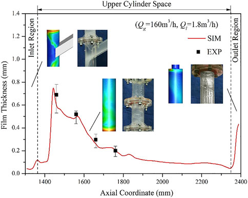
FIGURE 5. Verification of film thickness along the axial direction of GLCC cylinder.

Results and Discussion

In order to facilitate the analysis, this article defines four mathematical description methods for the thickness of the liquid film, the axial velocity of the liquid film, and the tangential velocity of the liquid film. They are the instantaneous value, the azimuth average value, the time average value, and the azimuth-time average value. Their definitions in the cylindrical coordinate system are expressed as

${\varphi }_{inst}=\varphi \left(R,\phi ,z,t\right),(9)$

${\varphi }_{azim}=\varphi \left(R,\overline{\phi },z,t\right),(10)$

${\varphi }_{time}=\varphi \left(R,\phi ,z,\overline{t}\right),(11)$

${\varphi }_{azim-time}=\varphi \left(R,\overline{\phi },z,\overline{t}\right).(12)$

The instantaneous value, ${\varphi }_{inst}$, can reflect the fluctuation and instability of the liquid film. The azimuthal mean, ${\varphi }_{azim}$, refers to the spatially averaged film properties along the circumference of the cylinder wall. The time-averaged value, ${\varphi }_{time}$, reflects the time-averaged characteristics of the liquid film over a period of time. The azimuth-time-averaged value, ${\varphi }_{azim-time}$, means that temporal fluctuations and circumferential spatial information are ignored, so it can reflect the overall distribution of the liquid film along the cylindrical wall.

Thickness of USLF Film

The azimuth-time average was used to describe the macroscopic distribution of USLF film thickness. Figure 6 shows the azimuth-time average film thickness at different axial heights under different gas–liquid flow rates. It can be seen that the simulation results agree well with the experimental results, especially when the gas flow rate is low or the liquid flow rate is low. Generally, the liquid film thickness value first increases rapidly and then decreases slowly along the axial direction. The liquid film at the inlet (indicated by the dotted line in the figure) is thin and has not yet formed. At 100mm–200 mm above the entrance (z=(1400–1600) mm, and the aspect ratio (z-z₀)/D=(1.2–3.9)), the thickness of the liquid film reaches the maximum, and its value can reach more than 1 mm. At the gas outlet (z = 2400 mm), the thickness of the liquid film increases sharply again due to the sudden contraction of the cylinder.

FIGURE 6

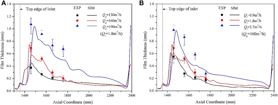
FIGURE 6. Axial distribution of USLF azimuth-time-averaged film thickness with (A) gas flow rates and (B) liquid flowrates.

In order to more intuitively understand the distribution law of the liquid film, the thickness of the liquid film under different gas–liquid flow rates is shown in Figure 7. In order to make the distribution more obvious, when the thickness of the liquid film is less than 0.2mm, it is a blank area. Considering the spatial properties of the swirl film, the back images (−90°–90°) and front images (90°–270°) of the cylinder are given, respectively.

FIGURE 7

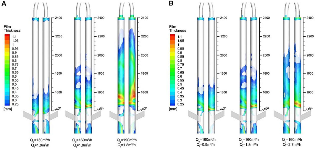
FIGURE 7. Contours of USLF film thickness distribution under different (A) gas flowrates and (B) liquid flowrates.

As shown in Figure 7, both the liquid film extension height and film thickness increase with the increase of gas flow rate or liquid flow rate. But they grow at slightly different rates. Liquid film thickness appears to be more sensitive to gas flow than to liquid flow. The reason can be explained from two aspects. On the one hand, the increase of gas flow velocity leads to the formation of annular flow in the inclined inlet pipe, which intensifies the occurrence of short-circuit membrane flow (① in Figure 2). On the other hand, the greater the gas flow rate, the stronger the ability of the gas flow to carry droplets, increasing the number of droplets directly brought into the upper space. In a word, the increase in the gas flow rate directly leads to the increase in the total amount of liquid brought into the upper cylinder, which is bound to have a greater impact on the flow pattern of the USLF.

Axial Velocity of USLF Film

Figure 8 shows the axial velocity distribution of the film under different gas–liquid flow rates. The cloud map only shows the area where the circumferential velocity of the liquid film is upward, and the area where the liquid film flows downward is blank. It can be seen that the greater the gas velocity, the greater the axial velocity of the liquid film at the inlet, and the direction of the liquid film velocity on the front and back sides seems to be generally opposite.

FIGURE 8

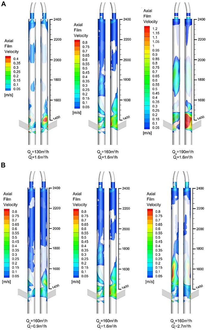
FIGURE 8. Contours of USLF axial film velocity under different (A) gas flowrates and (B) liquid flowrates.

Taking the working conditions of 160 m³/h-1.8 m³/h as an example, as shown in Figure 9, with the increase in height, the axial velocity rapidly drops to zero and fluctuates between positive and negative values. When the axial height exceeds 1400 mm, the axial velocity directions of the front and back sides of the USLF liquid film tend to be opposite. The reason is mainly related to the gas-phase flow field, that is, the vortex core of the swirl flow field is constantly shifting and swaying, which leads to a difference in the airflow shear force on the two side walls. The sheer force of the airflow on the wall near the vortex core is strong, causing the liquid film to rise. While the sheer force of the airflow near the wall on the far side of the vortex core is insufficient, so the liquid film falls downward.

FIGURE 9

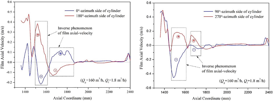
FIGURE 9. Film Axial Velocity at four azimuth of the cylinder for the gas–liquid flowrates of 160–1.8 m³/h.

The effect of gas flow rate or liquid flow rate on the axial velocity of the liquid film is shown in Figure 10. The azimuth-time average value is used for the axial velocity of the liquid film here. The axial velocity generally shows a trend of first positive and then negative. The axial flow direction of the film is initially positive (1360 mm < z < 1460 mm), and then the axial velocity decreases to a negative value (1460 mm < z < 1660 mm). The axial velocity becomes positive again later at high gas velocity (see the blue curve, Q_g = 190 m³/h, in the enlarged view in Figure 10A).

FIGURE 10

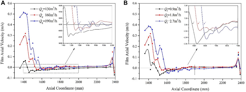
FIGURE 10. Axial distribution of USLF azimuth-time-averaged axial film velocity under different (A) gas flowrates and (B) liquid flowrates.

Figure 10B depicts the effect of different fluid volumes on the axial film velocity. Unlike the gas flow rate, the liquid film axial velocity becomes positive again at very low liquid flow rates (for example, Q_l = 0.9 m³/h) because the liquid film is lighter and easier to carry. However, when the liquid flow rate is large (for example, Q_l = 2.7 m³/h), due to the large gravity of the liquid film, it is difficult to pull the entire liquid film upward, so the axial velocity cannot be turned positive again.

Tangential Velocity of USLF Film

The film tangential velocity distributions under different gas–liquid conditions are shown in Figure 11 and Figure 12. It can be seen from Figure 11 that the tangential velocity increases first and then decreases with the height. The film tangential velocity is lower below z = 1400 mm. It increases sharply at z = 1400–1450 mm. Above z = 1450 mm, the film tangential velocity begins to decrease. After z = 1800 mm, the film tangential velocity decays to about 1/10 of the maximum tangential velocity. Figure 11 shows that the maximum tangential velocity mainly occurs at the axial position above the inlet at (z-z₀)/D = (0–3).

FIGURE 11

FIGURE 11. Contours of USLF axial film velocity under different (A) gas flow rates and (B) liquid flowrates.

FIGURE 12

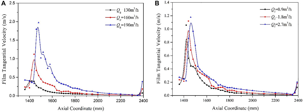
FIGURE 12. Axial distribution of USLF azimuth-time-averaged tangential film velocity under different (A) gas flow rates and (B) liquid flowrates.

Accordingly, the cylindrical space could be divided into two sections: 1) Liquid film swirling zone: When the aspect ratio (z-z₀)/D < 3, the liquid film mainly performs a swirling motion under the effects of the swirling gas flow field. 2) Liquid film churning zone: When the (z-z₀)/D > 3, the film moves almost axially and keeps churning upward and downward.

The effect of gas flowrates and liquid flowrates can be seen in Figure 12. The maximum value of tangential velocity increased with the growth of gas flowrates within this range of the gas flowrates. While as the liquid flow rate increases, it increases much less. This suggests that, in the range of gas–liquid flowrates involved in this article, the tangential velocity of the liquid film may be more sensitive to changes in the gas flowrates than the liquid flowrates. For higher gas flow rates, the attenuation of the film tangential velocity may be slowed down. This is because the liquid film almost forms a vertical annular flow and the swirl characteristics are weak, so the tangential velocity of the liquid film becomes not obvious. Therefore, the aforementioned rules might only apply when the USLF is still in the state of churn flow. When the USLF becomes a completely vertical annular flow, the tangential film velocity value is likely to be maintained or decreased.

Typical Distribution of USLF Film

The aforementioned analyses proved that there were differences and similarities in the flow characteristics of the USLF under different gas–liquid flow rates.

The distinction for the aforementioned five gas–liquid flowrates is reflected in the axial film velocity. For relatively low liquid flow rates, the axial film velocity was usually negative. For moderate gas–liquid flow rates, the axial film velocity changed its direction continuously. And for high gas flow rates, the axial film velocity was generally positive.

But whatever the flow regime it is, they have two obvious flow characteristics. First, without exception, the position (z_rev1) where the axial film velocity first intersected with the zero-line corresponded to the position (z_max) where the thickest liquid film was located. Second, the tangential film velocity had a strong synchronous relationship with the film thickness. Almost certainly, the thickest film would appear simultaneously with the maximum tangential film velocity. Both of these similarities and distinctions can be observed in Figures 6, 9, 12.

According to these key features, the typical shape and corresponding laws of the film thickness, the axial film velocity, and the tangential film velocity can be summarized in Figure 13.

FIGURE 13

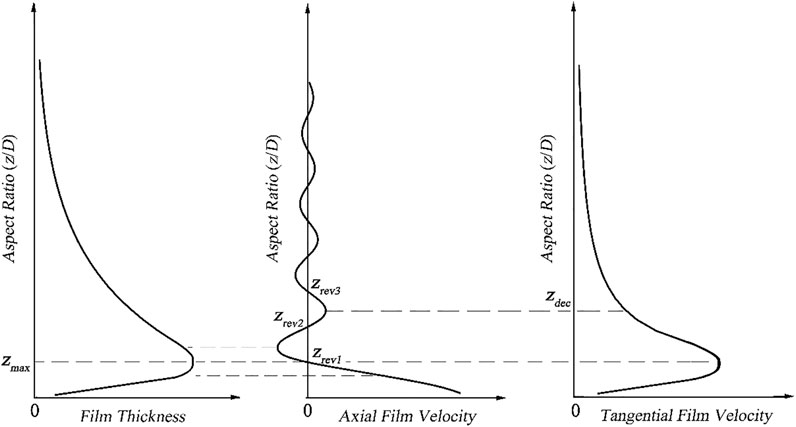
FIGURE 13. Typical distribution of USLF thickness, axial film velocity, and tangential film velocity.

Conclusion

The flow characteristics of Upper Swirling Liquid Film (USLF) were investigated via numerical simulation based on an improved Eulerian-EWF coupled method. Several conclusions are drawn as follows:

1) With an improved inlet boundary by profile-defined programming and the introduction of droplet size distribution by using the PBM model, the simulated flow characteristics of USLF agreed well with our measured results.

2) The distribution of film thickness, axial film velocity, and tangential film velocity of the USLF were obtained. Both the film thickness and the tangential film velocity had trends of increasing sharply at first and decreasing slowly at second, while the film axial velocity increased sharply and then dropped to zero followed by fluctuations. These flow parameters of USLF seem to be more sensitive to the gas flow rates than to the liquid flow rates.

3) The corresponding relationships of film thickness, axial velocity, and tangential velocity were analyzed for different gas–liquid flow rates. Two similarities between them were found: 1) the position of zero intersection of axial film velocity always corresponded to the position of the thickest liquid film, and 2) the attenuation process of tangential film velocity had a strong synchronous relationship with the film thickness. The typical shape and distribution of USLF parameters were summarized accordingly.

Data Availability Statement

The raw data supporting the conclusion of this article will be made available by the authors, without undue reservation.

Author Contributions

TY performed the data analysis and wrote the manuscript; JC contributed significantly to the conception and manuscript preparation; YW performed the experiment; FZ and XL helped perform the analysis with constructive discussions; LZ and SH contributed to the analysis of the study; and QS and SD edited the manuscript. All authors read and approved the final manuscript.

Conflict of Interest

The authors declare that the research was conducted in the absence of any commercial or financial relationships that could be construed as a potential conflict of interest.

Publisher’s Note

All claims expressed in this article are solely those of the authors and do not necessarily represent those of their affiliated organizations, or those of the publisher, the editors, and the reviewers. Any product that may be evaluated in this article, or claim that may be made by its manufacturer, is not guaranteed or endorsed by the publisher.

Acknowledgments

The authors acknowledge the financial support of the National Natural Science Foundation of China (No. 22078357), National Key Research and Development Plan (Grant Nos. 2018YFE0116100, 2018YFC0310504, and 2016YFC0303708) and Sichuan Science and Technology Program (Grant No. 2019ZDZX0001).

References

Ahmed, S., Soto, G. S., Naser, J., and Nakagawa, E. (2011). A Modified Eulerian-Lagrangian Approach Applied to a Compact Down-Hole Sub-sea Gas-Liquid Separator. Sep. Sci. Technol. 46 (4), 531–540. doi:10.1080/01496395.2010.531491

CrossRef Full Text | Google Scholar

Barnea, D. (1987). A Unified Model for Predicting Flow-Pattern Transitions for the Whole Range of Pipe Inclinations[J]. Int. J. Multiph. Flow, 1

CrossRef Full Text | Google Scholar

Chirinos, W. A., Gomez, L. E., and Wang, S. (2000). Liquid Carry-Over in Gas-liquid Cylindrical Cyclone Compact Separators[J]. SPE J. 5 (3), 259–267. doi:10.2118/65094-pa

CrossRef Full Text | Google Scholar

Ding, H., Sun, C., Wen, C., and Liang, Z. (2022). The Droplets and Film Behaviors in Supersonic Separator by Using Three-Field Two-Fluid Model with Heterogenous Condensation. Int. J. Heat Mass Transf. 184, 122315. doi:10.1016/j.ijheatmasstransfer.2021.122315

CrossRef Full Text | Google Scholar

Funahashi, H., Vierow Kirkland, K., Hayashi, K., Hosokawa, S., and Tomiyama, A. (2018). Interfacial and Wall Friction Factors of Swirling Annular Flow in a Vertical Pipe. Nucl. Eng. Des. 330, 97–105. doi:10.1016/j.nucengdes.2018.01.043

CrossRef Full Text | Google Scholar

Hreiz, R., Lainé, R., Wu, J., Lemaitre, C., Gentric, C., and Fünfschilling, D. (2014). On the Effect of the Nozzle Design on the Performances of Gas-Liquid Cylindrical Cyclone Separators. Int. J. Multiph. Flow 58, 15–26. doi:10.1016/j.ijmultiphaseflow.2013.08.006

CrossRef Full Text | Google Scholar

Kataoka, H., Shinkai, Y., and Tomiyama, A. (2009). Pressure Drop in Two-phase Swirling Flow in a Steam Separator. Jpes 3 (2), 382–392. doi:10.1299/jpes.3.382

CrossRef Full Text | Google Scholar

Li, J., Zheng, W., and Hong, F. (2021). Three-Dimensional Lattice Boltzmann Investigation on Pore Scale Liquid‐Vapor Distribution Patterns and Heat Transfer Performance of a Loop Heat Pipe Heterogeneous Porous Wick Evaporator[J]. Int. Commun. Heat Mass Transf. 128, 105639. doi:10.1016/j.icheatmasstransfer.2021.105639

CrossRef Full Text | Google Scholar

Liu, W., and Bai, B. (2015). A Numerical Study on Helical Vortices Induced by a Short Twisted Tape in a Circular Pipe. Case Stud. Therm. Eng. 5, 134–142. doi:10.1016/j.csite.2015.03.003

CrossRef Full Text | Google Scholar

Min, L. I., Hongguang, Z., and Qinghua, G. U. (2015). “Numerical Simulation on Water Film Condensed on Stack Inner Wall of "near Zero" Emissions Power Plants[J],” in Thermal Power Generation.

Google Scholar

Paz, C., Suárez, E., Parga, O., and Vence, J. (2017). Glottis Effects on the Cough Clearance Process Simulated with a CFD Dynamic Mesh and Eulerian Wall Film Model. Comput. Methods Biomechanics Biomed. Eng. 20 (12), 1326–1338. doi:10.1080/10255842.2017.1360872

PubMed Abstract | CrossRef Full Text | Google Scholar

Punekar, H., Ingle, R., and Cao, J. (2014). “Modeling of Particle Wall Interaction and Film Transport Using Eulerian Wall Film Model,” in ASME 2014 Gas Turbine India Conference, V001T03A006.

CrossRef Full Text | Google Scholar

Taitel, Y., and Dukler, A. E. (1976). A Model for Predicting Flow Regime Transitions in Horizontal and Near Horizontal Gas-Liquid Flow[J]. AIChE J. 47.

Google Scholar

Ti, Y. (2019). Gas-liquid Flow Behavior and Separation Mechanism for the Upper Cylinder in Gas-liquid Cylindrical Cyclone[D]. Beijing: China University of Petroleum, 53.

Google Scholar

Ti, Y., Jianyi, C., and Jianfei, S. (2019). Experimental and Numerical Study of Upper Swirling Liquid Film (USLF) Among Gas-Liquid Cylindrical Cyclones (GLCC)[J]. Chem. Eng. J. 358, 806.

Google Scholar

Xiong, Z., Lu, M., Wang, M., Gu, H., and Cheng, X. (2014). Study on Flow Pattern and Separation Performance of Air-Water Swirl-Vane Separator. Ann. Nucl. Energy 63, 138–145. doi:10.1016/j.anucene.2013.07.026

CrossRef Full Text | Google Scholar

Yajun, D., Lin, Z., and Hao, H. (2019). Modeling and Simulation of the Gas-Liquid Separation Process in an Axial Flow Cyclone Based on the Eulerian-Lagrangian Approach and Surface Film Model[J]. Power Technol. 353, 473. doi:10.1016/j.powtec.2019.05.039

CrossRef Full Text | Google Scholar

Yang, J., Zhang, X., Shen, G., Xiao, J., and Jin, Y. (2015). Modeling the Mean Residence Time of Liquid Phase in the Gas-Liquid Cyclone. Ind. Eng. Chem. Res. 54 (43), 10885–10892. doi:10.1021/acs.iecr.5b02617

CrossRef Full Text | Google Scholar

Ying, X. U., Rong, J., and Tao, Z. (2016). Research on Two-phase Flow Model for Wet Gas Based on Venturi Flow sensor[J]. Tianjin: Transducer and Microsystem Technologies.

Google Scholar