Prediction of wax deposit thickness in waxy crude oil pipelines using improved GM(1,1) model

In this paper, the GM(1,1) model with function $\arccos \left(x\right)$ transformation and GM(1,1) model with function transformation are established by using arccosine function transformation method and $a^{\arccos \left(x\right)}$ function transformation method, and the GM(1,1) model with function $\cos \left(x^2\right)$ transformation is established by using function transformation theory, and GM(1,1) model with function $\cos \left(x^2+c\right)$ transformation is established by using translational transformation theory on the basis of this model. The prediction accuracy of GM(1,1) model, GM(1,1) model with function $\arccos \left(x\right)$ transformation, GM(1,1) model with function $a^{\arccos \left(x\right)}$ transformation, GM(1,1) model with function $\cos \left(x^2\right)$ transformation, and GM(1,1) model with function $\cos \left(x^2+c\right)$ transformation are compared by modeling with the field pipeline data and the indoor loop data. The influence of $a$ value in GM(1,1) model with function $a^{\arccos \left(x\right)}$ transformation on prediction accuracy is discussed, and the influence of $c$ value in GM(1,1) model with function $\cos \left(x^2+c\right)$ transformation on prediction accuracy is discussed. With the increase of $a$ and $c$ values, the average relative error show a trend of decreasing and then increasing, by comparing the average relative errors under different $a$ and $c$ values, the optimal a value and c value and the optimal prediction accuracy are obtained. The results show that the GM(1,1) model with function $\cos \left(x^2+c\right)$ transformation in the indoor loop has an average relative error of 0.6490% when $c=0.114$, which is the minimum average relative error compared to other models and achieves the highest prediction accuracy. The GM(1,1) model with function $\cos \left(x^2+c\right)$ transformation in the field pipeline has an average relative error of 1.94156% when $c=-0.555$, which is the minimum average relative error compared to other models and achieves the highest prediction accuracy. Among the five models, only the GM(1,1) model with function $\cos \left(x^2+c\right)$ transformation has fitted and predicted values that are closer to the actual thickness values in the indoor loop experimental data and the field pipeline data, and the predicted values are more consistent with the actual conditions in the field pipeline. This paper verifies the feasibility of using the GM(1,1) model with function $\cos \left(x^2+c\right)$ transformation to predict the wax deposition thickness of the pipe wall, and provides a reference for subsequent research on accurate prediction of wax deposition thickness.

1 Introduction

When the temperature of crude oil containing wax is lower than the waxing point, the dissolved wax crystals will be deposited on the inner wall of the pipe; as the thickness of wax deposition increases, the pipe diameter decreases, the transmission capacity decreases, and the energy consumption increases (Alnaimat et al., 2020; Ridzuan et al., 2020; Zhou et al., 2016). In order to ensure the efficient and safe operation of the pipeline, regular pipe cleaning is adopted to reduce the wax deposition thickness. In the process of developing the pipe cleaning cycle, mastering the wax deposition law and accurately predicting the thickness of wax deposition are the prerequisites for developing the pipe cleaning cycle (Li et al., 2020; Duan et al., 2016). Over time, the wax deposit thickness will tend to grow, and shear stripping will occur after the wax deposit grows to a certain thickness. Lu et al. (Lu et al., 2012) proposed that there are three effects that affect the increase or decrease of wax deposition, and the wax deposition decreases with the increase of flow rate by flow loop device experiments. Jin et al. (Jin et al., 2018) analyzed the trend of wax deposition thickness under different time periods, divided the wax deposition process into three stages: rapid deposition, faster deposition, and slow deposition, and verified the feasibility of the model; the model is highly accurate and has good application value. Wang et al. (Wang et al., 2016) developed a wax deposition thickness prediction and economic pipe cleaning cycle prediction program for the Tieling-Xinmin section of the pipeline as an example, and the prediction effect of this program is more consistent with the actual thickness value of the pipeline in the field, and the program can only predict one-quarter at present. Leporini et al. (Leporini et al., 2019) fitted the laboratory wax deposition data with a mathematical model, and to verify the error of the predicted values of the mathematical model, the data were scaled up and compared with the field data in the oil field. It is finally concluded that the shear stripping mechanism must be initiated in the multiphase flow simulation. Jalalnezhad et al. (Jalalnezhad et al., 2016) developed the ANFIS model from experimental data, and the predictions of this model were closer to the experimental data. The ANFIS model was more accurate than the Halstensen model in predicting wax deposition thickness at single-phase turbulent flow rates. Saeedi Dehaghani et al. (Saeedi et al., 2017) developed an artificial neural network model (ANN) to predict the wax deposition thickness in single-phase turbulent flow and the ANN model was compared with the ANFIS model and the predicted values of the ANN model were closer to the experimental data. Alnaimat et al. (Alnaimat et al., 2020) comprehensively evaluated different techniques for wax deposition thickness prediction and compared with other models, the Matzain model gave better results for wax deposition thickness prediction, therefore, the optimized Matzain model can be studied in more depth. Gray system theory is the study of the exploitation of a small sample of partially known information to achieve the correct description and effective monitoring of evolutionary laws in the presence of a large lack or disorder of information (Julong., 1989). Scholars often refer to the GM(1,1) model in the gray model to predict the wax deposition thickness. While the traditional GM(1,1) model has some limitations, if the smoothness of the original series is low or there are extreme values, it will have a serious impact on the prediction accuracy.

In order to improve the prediction accuracy of the GM(1,1) model, researchers have improved the traditional GM(1,1) model. Wang et al. (Wang et al., 2014) established a new model by optimizing the background values in the gray model, and compared with the traditional GM(1,1) model, the new model has higher prediction accuracy. Xu et al. (Xu et al., 2021) used the function $\cot \left(x^2+c\right)$ transformation to build a new GM(1,1) model, and verified that the model has higher prediction accuracy than the function $\cot \left(x^2\right)$ transformation model. Jin et al. (Jin et al., 2022) introduced logarithmic function transformation and translation transformation in the modeling steps of traditional GM(1,1) model to establish a new model. The accuracy of the improved model is higher than that of the traditional GM(1,1) model, and the reasonable translation variables make the improved GM(1,1) model have higher prediction accuracy. Literatures (Xu et al., 2021; Jin et al., 2022; Zhang et al., 2016; Huanyong et al., 2007; Liu et al., 2013; Shao et al., 2010; Yao-guo et al., 2009) proposed the cotangent function transformation, logarithmic function transformation, inverse cotangent function transformation, exponential logarithmic function transformation, cosine function transformation, sine function transformation, and linear transformation to improve the smoothness of the original sequence and thus improve the model prediction accuracy, respectively.

In order to make the prediction of wax deposition thickness more accurate, new function transformations are proposed in this paper. The GM(1,1) model with function $\arccos \left(x\right)$ transformation and the GM(1,1) model with function $a^{\arccos \left(x\right)}$ transformation are established by using the arccosine function transformation method and the $a^{\arccos \left(x\right)}$ function transformation method, and the GM(1,1) model with function $\cos \left(x^2\right)$ transformation is established by using the function transformation theory, and the GM(1,1) model with function $\cos \left(x^2+c\right)$ transformation is established by using the translational transformation theory on the basis of this model.

2 Establish the model

The prediction principle of GM(1,1) model is to generate a new set of data series with obvious trend for a certain data series by accumulation, build a model for prediction according to the growth trend of the new data series, and then reverse the calculation by accumulation and subtraction to recover the original data series, and then get the prediction result.

2.1 Establish GM(1,1) model

1) Original data sequence:

$X^{\left(0\right)}=\left\{x^{\left(0\right)}\left(1\right),x^{\left(0\right)}\left(2\right),\cdots ,x^{\left(0\right)}\left(n\right)\right\}(1)$

Where: $x^{\left(0\right)}\left(k\right)>0$, $k=\mathrm{1,2},\cdots n.$

2) Accumulate the data sequence $X^{\left(0\right)}$ to generate sequence $X^{\left(1\right)}$:

$X^{\left(1\right)}=\left\{x^{\left(1\right)}\left(1\right),x^{\left(1\right)}\left(2\right),\cdots ,x^{\left(1\right)}\left(n\right)\right\}(2)$

Where: $x^{\left(1\right)}\left(k\right)={\displaystyle \sum }_{k=1}^n{x}^{\left(0\right)}\left(k\right)$, $k=\mathrm{1,2},\cdots ,n.$

3) Generate mean sequence:

$Z^{\left(1\right)}\left(k\right)=a{x}^{\left(1\right)}\left(k\right)+\left(1-a\right)x^{\left(1\right)}\left(k-1\right)(3)$

Where: $0\le a\le 1$, $a$ is generally taken as 0.5, $k=\mathrm{2,3},\cdots ,n.$

4) Establish the GM(1,1) model whitening differential equation:

$\frac{d{x}^{\left(1\right)}}{dt}+a{x}^{\left(1\right)}=b(4)$

5) Establish the GM(1,1) model gray differential equation:

$x^{\left(0\right)}\left(k\right)+a{Z}^{\left(1\right)}\left(k\right)=b(5)$

Where: $k=\mathrm{2,3},\cdots ,n.a$ is the system development coefficient, $b$ is gray action quantity.

$a,b$ is obtained by the following least squares method:

$\phi =\left[\begin{array}{c}a\\ b\end{array}\right]={\left[\begin{array}{cc}{B}^T& B\end{array}\right]}^{-1}{B}^{T}Y(6)$

Where: $B=\left[\begin{array}{cc}\begin{array}{c}-Z^{\left(1\right)}\left(2\right)\\ \begin{array}{c}\begin{array}{c}-Z^{\left(1\right)}\left(3\right)\\ ⋮\end{array}\\ -Z^{\left(1\right)}\left(n\right)\end{array}\end{array}& \begin{array}{c}\begin{array}{c}\begin{array}{c}1\\ 1\end{array}\\ ⋮\end{array}\\ 1\end{array}\end{array}\right]$, $Y=\left[\begin{array}{c}{x}^{\left(0\right)}\left(2\right)\\ x^{\left(0\right)}\left(3\right)\\ ⋮\\ x^{\left(0\right)}\left(n\right)\end{array}\right]$.

6) The time response sequence equation is obtained by solving:

${\stackrel{⌢}{x}}^{\left(1\right)}\left(k\right)=\left[x^{\left(0\right)}\left(1\right)-\frac{b}{a}\right]e^{-a\left(k-1\right)}+\frac{b}{a}(7)$

Where: $k=\mathrm{2,3},\cdots ,n.$

7) Reduction yields the model prediction sequence equation:

${\stackrel{⌢}{x}}^{\left(0\right)}\left(k\right)={\stackrel{⌢}{x}}^{\left(1\right)}\left(k\right)-{\stackrel{⌢}{x}}^{\left(1\right)}\left(k-1\right)=\left(1-e^a\right)\left[x^{\left(0\right)}\left(1\right)-\frac{b}{a}\right]e^{-a\left(k-1\right)}(8)$

Where: $k=\mathrm{2,3},\cdots ,n$. When $k=1$ the GM(1,1) model predicted values are consistent with the original data.

2.2 Establish the GM(1,1) model for the transformation of function $\arccos \left(x\right)$ and function $a^{\arccos \left(x\right)}$

The function $\arccos \left(x\right)$ transformation method can improve the sequence smoothness and make the prediction accuracy of this model more accurate. The specific modeling process is as follows:

1) Set the original sequence $A^{\left(0\right)}=\left\{a^{\left(0\right)}\left(1\right),a^{\left(0\right)}\left(2\right),\cdots ,a^{\left(0\right)}\left(n\right)\right\}$, $a^{\left(0\right)}\left(k\right)>0$, $k=\mathrm{1,2},\cdots ,n.$ Standardize the original data sequence, the new sequence is shown in Eq. 9:

$X^{\left(0\right)}=\left\{x^{\left(0\right)}\left(1\right),x^{\left(0\right)}\left(2\right),\cdots ,x^{\left(0\right)}\left(n\right)\right\}(9)$

Where: $x^{\left(0\right)}\left(k\right)=a^{\left(0\right)}\left(k\right)/c$, $c$ is a constant number, $0<x^{\left(0\right)}k<1$, $k=\mathrm{1,2},\cdots ,n.$

2) The sequence $X^{\left(0\right)}$ is transformed by the function $\arccos \left(x\right)$ to obtain the sequence $Y^{\left(0\right)}$ as shown in Eq. 10:

$Y^{\left(0\right)}=\left\{y^{\left(0\right)}\left(1\right),y^{\left(0\right)}\left(2\right),\cdots ,y^{\left(0\right)}\left(n\right)\right\}(10)$

Where: $y^{\left(0\right)}\left(k\right)=\arccos x^{\left(0\right)}\left(k\right)$, $k=\mathrm{1,2},\cdots ,n.$

3) The sequence $y^{\left(0\right)}\left(k\right)$ is obtained and then modeled according to the GM(1,1) model to obtain the final predicted sequence ${\stackrel{⌢}{x}}^{\left(0\right)}\left(k\right)$, and the predicted sequence ${\stackrel{⌢}{x}}^{\left(0\right)}\left(k\right)$ is reduced:

${\stackrel{⌢}{x}}^{\left(0\right)}\left(k\right)=\cos {\stackrel{⌢}{y}}^{\left(0\right)}\left(k\right)(11)$

Where: $k=\mathrm{1,2},\cdots ,n.$

4) Then reduce ${\stackrel{⌢}{x}}^{\left(0\right)}\left(k\right)$ to $a^{\left(0\right)}\left(k\right)$ , and $a^{\left(0\right)}\left(k\right)$ is the final predicted value.

5) The modeling process for the GM(1,1) model with function $a^{\arccos \left(x\right)}$ transformation is the same as above, and the reduced formula of this model is shown in Eq. 12 and Eq. 13:

$y^{\left(0\right)}\left(k\right)=a^{\arccos x^{\left(0\right)}\left(k\right)}(12)$

${\stackrel{⌢}{x}}^{\left(0\right)}\left(k\right)=\cos \left({\log }_a^{\widehat{y}{\left(0\right)}_{\left(k\right)}}\right)(13)$

2.3 Establish the GM(1,1) model for the transformation of function $\cos \left(x^2\right)$ and function $\cos \left(x^2+c\right)$

In the literature (Liu et al., 2013), it was demonstrated theoretically that the smoothness of the original data series can be elevated when the function $\cos \left(x^2\right)$ is transformed in the $1<x<\sqrt{\pi /2}$ interval, which makes the prediction accuracy of this model more accurate. The specific modeling process is as follows:

1) Set the original sequence $A^{\left(0\right)}=\left\{a^{\left(0\right)}\left(1\right),a^{\left(0\right)}\left(2\right),\cdots ,a^{\left(0\right)}\left(n\right)\right\}$, $y^{\left(0\right)}\left(k\right)>0$, $k=\mathrm{1,2},\cdots ,n.$ The original data series is normalized to obtain the new series as shown in Eq. 14:

$X^{\left(0\right)}=\left\{x^{\left(0\right)}\left(1\right),x^{\left(0\right)}\left(2\right),\cdots ,x^{\left(0\right)}\left(n\right)\right\}(14)$

where $1<y^{\left(1\right)}\left(k\right)<\sqrt{\pi /2}$, $k=\mathrm{1,2},\cdots ,n.$

2) The sequence $Y^{\left(0\right)}$ obtained by performing function $\cos \left(x^2\right)$ transformation on the sequence $X^{\left(0\right)}$ is shown in Eq. 15:

$Y^{\left(0\right)}=\left\{y^{\left(0\right)}\left(1\right),y^{\left(0\right)}\left(2\right),\cdots ,y^{\left(0\right)}\left(n\right)\right\}(15)$

Where: $y^{\left(0\right)}\left(k\right)=\cos \left[\left(x^{\left(0\right)}\left(k\right){)}^2\right.\right]$.

3) The sequence $y^{\left(0\right)}\left(k\right)$ is obtained and then modeled according to the GM(1,1) model to obtain the final predicted sequence ${\stackrel{⌢}{x}}^{\left(0\right)}\left(k\right)$, and the predicted sequence ${\stackrel{⌢}{x}}^{\left(0\right)}\left(k\right)$ is reduced:

${\stackrel{⌢}{x}}^{\left(0\right)}\left(k\right)=\sqrt{\arccos {\stackrel{⌢}{y}}^{\left(0\right)}\left(k\right)}(16)$

4) Then reduce ${\stackrel{⌢}{x}}^{\left(0\right)}\left(k\right)$ to $a^{\left(0\right)}\left(k\right)$ , and $a^{\left(0\right)}\left(k\right)$ is the final predicted value.

5) The modeling process for the GM(1,1) model with function $\cos \left(x^2+c\right)$ transformation is the same as above, and the reduction formula of this model is shown in Eq. 17 and Eq. 18:

$y^{\left(0\right)}\left(k\right)=\cos \left[\left(x^{\left(0\right)}{\left(k\right))}^2+c\right.\right](17)$

${\stackrel{⌢}{x}}^{\left(0\right)}\left(k\right)=\sqrt{\arccos {\stackrel{⌢}{y}}^{\left(0\right)}\left(k\right)-c}(18)$

3 Calculation example

To verify the accuracy of the models, GM(1,1) model, GM(1,1) model with function $\arccos \left(x\right)$ transformation, GM(1,1) model with function $a^{\arccos \left(x\right)}$ transformation, GM(1,1) model with function $\cos \left(x^2\right)$ transformation, and GM(1,1) model with function $\cos \left(x^2+c\right)$ transformation were established with indoor loop waxing experiments and field pipeline data, and the average relative errors of the five models were analyzed.

3.1 Wax deposition thickness prediction model for indoor loop experiments

The indoor loop device can simulate the wax deposition phenomenon in the field pipeline more realistically. In the literature (Chen et al., 2015), an indoor loop experimental device was used to simulate the wax formation in the pipeline at different inlet fluid temperatures, and then the wax formation thickness of the pipe wall was calculated using the static differential pressure method. The wax deposition thickness data in the pipe at the inlet fluid temperature of 50°C in the literature (Chen et al., 2015) was taken as an example, and since the thickness was 0 for the first 4 h, the wax deposition thickness from 5 h to 10 h was used as the base data for modeling and prediction of the thickness within 11 h to 12 h. The standardized data for the GM(1,1) model with function $\arccos \left(x\right)$ transformation and the GM(1,1) model with function $a^{\arccos \left(x\right)}$ transformation are shown in Table 1:

TABLE 1

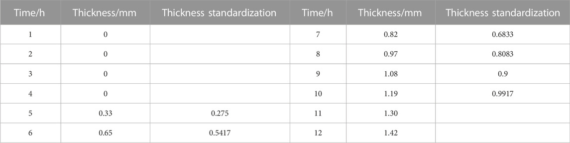
TABLE 1. Standardized data for the GM(1, 1) model with function $\arccos \left(x\right)$ and $a^{\arccos \left(x\right)}$ transformations in the indoor loop.

After obtaining the standardized data, GM(1,1) model, GM(1,1) model with function $\arccos \left(x\right)$ transformation, and GM(1,1) model with function $a^{\arccos \left(x\right)}$ transformation are established respectively, and the specific prediction sequence equations are shown in Table 2, and the predicted results of wax deposition thickness are shown in Table 3, and the comparison between the predicted and actual values is shown in Figure 1.

TABLE 2

TABLE 2. Prediction sequence formula for GM(1,1) model and GM(1,1) model with function $\arccos \left(x\right)$ and $a^{\arccos \left(x\right)}$ transformations in the indoor loop.

TABLE 3

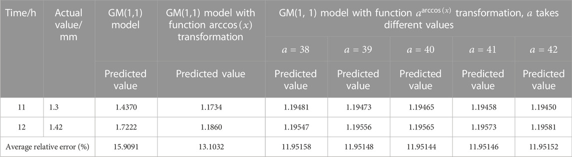
TABLE 3. Comparison of wax deposition thickness prediction results of GM(1,1) model and GM(1,1) model with function $\arccos \left(x\right)$ and $a^{\arccos \left(x\right)}$ transformations in the indoor loop.

FIGURE 1

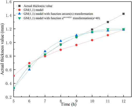
FIGURE 1. Comparison of predicted and actual values of wax deposition thickness for GM(1,1) model and GM(1,1) model with function $\arccos \left(x\right)$ and $a^{\arccos \left(x\right)}$ transformations in the indoor loop.

According to the results in Table 3, it can be found that the average relative errors of all three models are relatively large. In the GM(1,1) model with function $a^{\arccos \left(x\right)}$ transformation, although the average relative error is the smallest at $a=40$, different $a$ values have almost no effect on the average relative error. In Figure 1, 5–8 h are the fitted values and 11–12 h are the predicted values. From Figure 1, it can be found that the fitted values of the GM(1,1) model with function $\arccos \left(x\right)$ transformation and the GM(1,1) model with function $a^{\arccos \left(x\right)}$ transformation are closer to the actual thickness values, while the predicted values have a large deviation from the actual thickness values. The accuracy of wax deposition thickness prediction of these three models in the indoor loop experiments is poor, and the predicted values of wax deposition thickness deviate from the experimental data, so it is not recommended to use these three models for predicting wax deposition thickness in the indoor loop experiments.

The standardized data for the GM(1,1) model with function $\cos \left(x^2\right)$ transformation and the GM(1,1) model with function $\cos \left(x^2+c\right)$ transformation are shown in Table 4:

TABLE 4

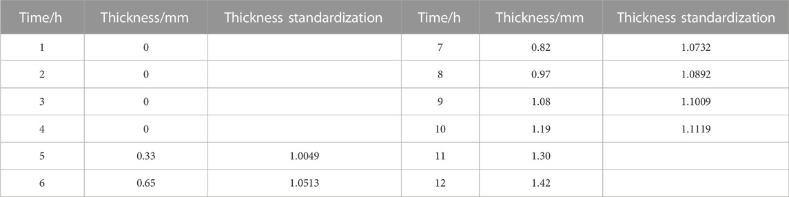
TABLE 4. Standardized data for GM(1,1) model with function $\cos \left(x^2\right)$ and $\cos \left(x^2+c\right)$ transformations in the indoor loop.

After obtaining the standardized data, GM(1,1) model, GM(1,1) model with function $\cos \left(x^2\right)$ transformation, and GM(1,1) model with function $\cos \left(x^2+c\right)$ transformation were established respectively, and the specific prediction sequence equations are shown in Table 5, and the predicted results of wax deposition thickness are shown in Table 6; the comparison between the predicted and actual values is shown in Figure 2.

TABLE 5

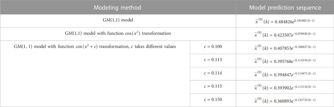
TABLE 5. Prediction sequence equation for GM(1,1) model and GM(1,1) model with function $\cos \left(x^2\right)$ and $\cos \left(x^2+c\right)$ transformations in the indoor loop.

TABLE 6

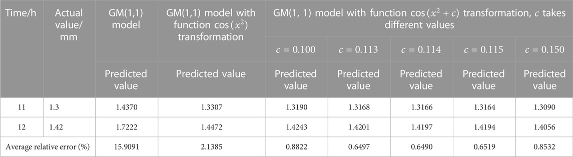
TABLE 6. Comparison of wax deposition thickness prediction results of GM(1,1) model and GM(1,1) model with function $\cos \left(x^2\right)$ and $\cos \left(x^2+c\right)$ transformations in the indoor loop.

FIGURE 2

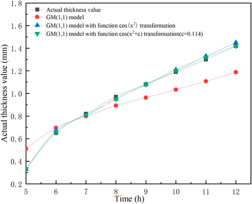
FIGURE 2. Comparison of predicted and actual values of wax deposition thickness for GM(1,1) model and GM(1,1) model with function $\cos \left(x^2\right)$ and $\cos \left(x^2+c\right)$ transformations in the indoor loop.

According to the results in Table 6, it can be found that the average relative error of wax deposition thickness shows a trend of decreasing and then increasing for different values of translation $c$ in the GM(1,1) model with function $\cos \left(x^2+c\right)$ transformation, indicating that the interval series is first standardized and then translation transformed, which finally improves the smoothness of the interval series. The average relative error of this model is 0.6490% when the translation $c=0.114$, which is the minimum average relative error value. The average relative error of the model suddenly becomes larger when the translation $c=0.2$, because $x^2+c>\pi /2$, which does not meet the specified interval $1<x^2+c<\pi /2$. The interval $1<x^2+c<\pi /2$ needs to be satisfied when the value of the translation $c$ is taken, and it is meaningless if the interval is exceeded. The average relative error of the GM(1,1) model with function $\cos \left(x^2\right)$ transformation is 2.1385%, while the average relative error of the GM(1,1) model is 15.9091%. Therefore, it is concluded that the GM(1,1) model with function $\cos \left(x^2+c\right)$ transformation has small average relative error and high prediction accuracy, the GM(1,1) model with function $\cos \left(x^2\right)$ transformation has the second highest prediction accuracy, while the GM(1,1) model has the lowest prediction accuracy. In Figure 2, 5 h∼8 h are the fitted values and 11 h∼12 h are the predicted values. The actual thickness values are closer to the fitted and predicted values of the GM(1,1) model with function $\cos \left(x^2+c\right)$ transformation, which indicates that the model is effective, has high prediction accuracy and is more in line with the actual situation. In contrast, the fitted and predicted values of the GM(1,1) model and the GM(1,1) model with function $\cos \left(x^2\right)$ transformation compared to the actual thickness values have large deviations, and the model effect is not satisfactory. The model based on the experimental data of the indoor loop can provide a reference for the theoretical study of predicting wax deposition thickness.

3.2 Wax deposit thickness prediction model for field pipelines

In order to make the predicted wax deposition thickness of the improved model more consistent with the actual situation in the field pipeline, the wax deposition thickness data of a field pipeline in the literature (Xu et al., 2021) is taken as an example in this paper, and the wax deposition thickness of 1 day∼15 days is used as the base data for modeling to predict the wax deposition thickness of 18 days∼21 days. The standardized data for the GM(1,1) model, the GM(1,1) model with function $\arccos \left(x\right)$ transformation, and the GM(1,1) model with function $a^{\arccos \left(x\right)}$ transformation are shown in Table 7.

TABLE 7

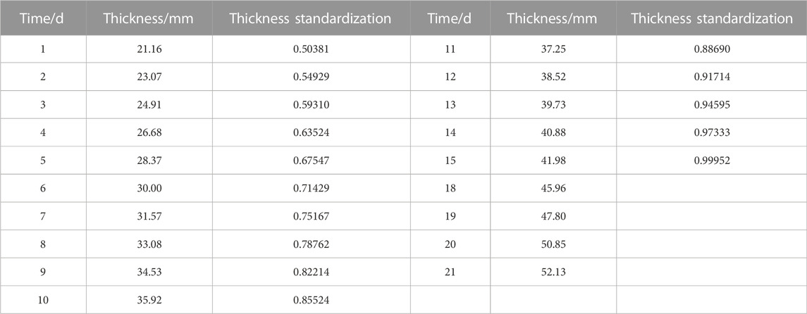
TABLE 7. Standardized data for the GM(1,1) model with functions $\arccos \left(x\right)$ and $a^{\arccos \left(x\right)}$ transformation in the field pipeline.

After obtaining the standardized data, the GM(1,1) model, GM(1,1) model with function $\arccos \left(x\right)$ transformation, and GM(1,1) model with function $a^{\arccos \left(x\right)}$ transformation were established respectively, and the specific prediction sequence equations are shown in Table 8, and the predicted results of wax deposition thickness are shown in Table 9, and the comparison between the predicted and actual values is shown in Figure 3.

TABLE 8

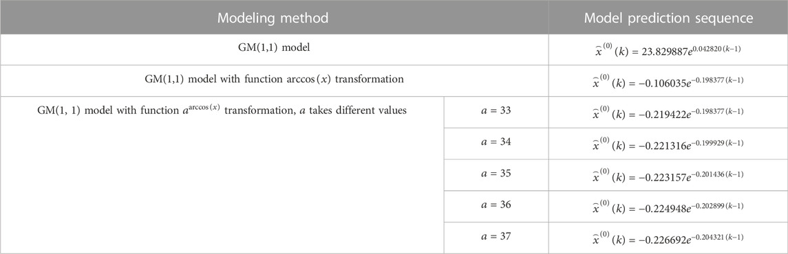
TABLE 8. Prediction sequence equation for GM(1,1) model and GM(1,1) model with function $\arccos \left(x\right)$ and $a^{\arccos \left(x\right)}$ transformations in the field pipeline.

TABLE 9

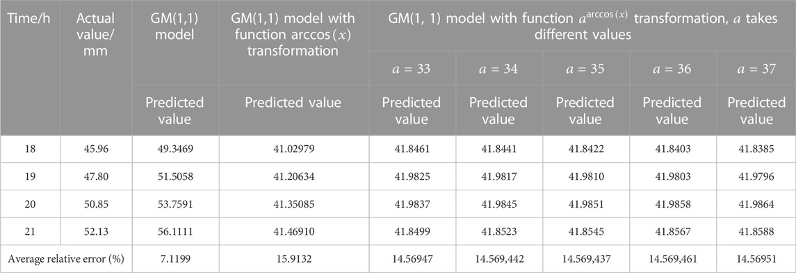
TABLE 9. Comparison of wax deposition thickness prediction results of GM(1,1) model and GM(1,1) model with function $\arccos \left(x\right)$ and $a^{\arccos \left(x\right)}$ transformations in field pipeline.

FIGURE 3

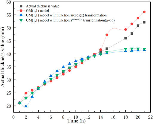
FIGURE 3. Comparison of predicted and actual values of wax deposition thickness for GM(1,1) model and GM(1,1) model transformed by functions $\arccos \left(x\right)$ and $a^{\arccos \left(x\right)}$ in the field pipeline.

According to the results in Table 9, the average relative error of the GM(1,1) model is 7.1199%, which is the minimum average relative error value. In the GM(1,1) model with the function $a^{\arccos \left(x\right)}$ transformation, the average relative error tends to decrease and then increase when different $a$ values are taken. When $a=35$, the average relative error is 14.569,437%, while the average relative error of the GM(1,1) model with function $\arccos \left(x\right)$ transformation is 15.9132%. Therefore, it is concluded that the GM(1,1) model has a small average relative error and high prediction accuracy, the GM(1,1) model with function $a^{\arccos \left(x\right)}$ transformation has the second highest prediction accuracy, and the GM(1,1) model with function $\arccos \left(x\right)$ transformation has the minimum prediction accuracy. In Figure 3, 1 day∼15 days are the fitted values and 18 days∼21 days are predicted values. The fitted and predicted values of the GM(1,1) model are closer to the actual thickness values, which indicates that the GM(1,1) model works well. The predicted values of the GM(1,1) model with function $\arccos \left(x\right)$ and $a^{\arccos \left(x\right)}$ transformations have large deviations from the actual thickness values, indicating that the prediction accuracy of the GM(1,1) model with function $\arccos \left(x\right)$ and $a^{\arccos \left(x\right)}$ transformations is poor; the model effect is not ideal and does not match the actual situation.

The standardized data for the GM(1,1) model with function $\cos \left(x^2\right)$ transformation and the GM(1,1) model with function $\cos \left(x^2+c\right)$ transformation are shown in Table 10:

TABLE 10

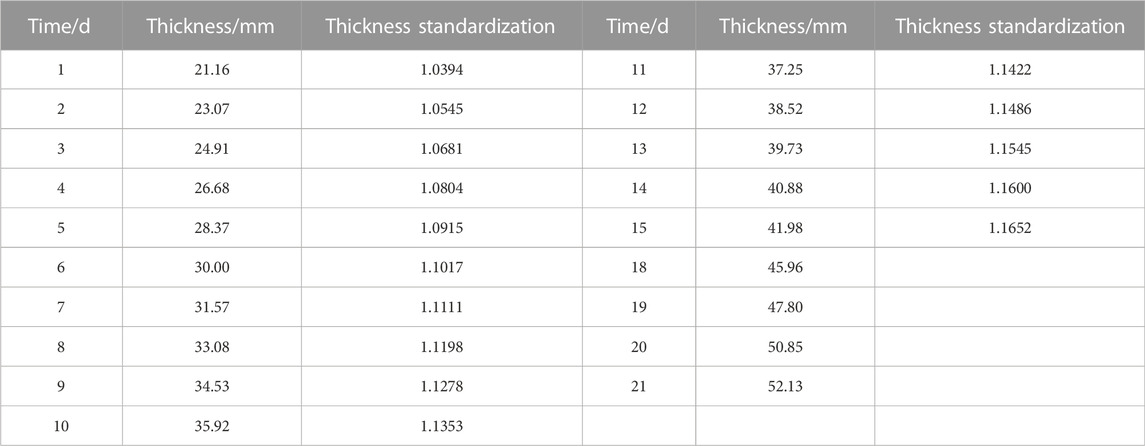
TABLE 10. Standardized data for the GM(1,1) model with function $\cos \left(x^2\right)$ and $\cos \left(x^2+c\right)$ transformations in the field pipeline.

After obtaining the standardized data, GM(1,1) model, GM(1,1) model with function $\cos \left(x^2\right)$ transformation, and GM(1,1) model with function $\cos \left(x^2+c\right)$ transformation were established respectively, and the specific prediction sequence equations are shown in Table 11, and the predicted results of wax deposition thickness are shown in Table 12, and the comparison between the predicted and actual values is shown in Figure 4.

TABLE 11

TABLE 11. Prediction sequence equation for GM(1,1) model and GM(1,1) model with function $\cos \left(x^2\right)$ and $\cos \left(x^2+c\right)$ transformations in the field pipeline.

TABLE 12

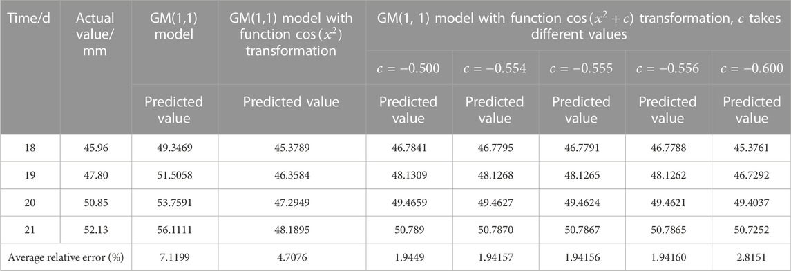
TABLE 12. Comparison of wax deposition thickness prediction results of GM(1,1) model and GM(1,1) model with function $\cos \left(x^2\right)$ and $\cos \left(x^2+c\right)$ transformations in the field pipeline.

FIGURE 4

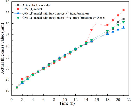
FIGURE 4. Comparison of predicted and actual values of wax deposition thickness for GM(1,1) model and GM(1,1) model with function $\cos \left(x^2\right)$ and $\cos \left(x^2+c\right)$ transformations in the field pipeline.

According to the results in Table 12, the average relative error in the GM(1,1) model with function $\cos \left(x^2+c\right)$ transformation is 1.94156% when the translation $c=-0.555$, which is the minimum average relative error value. The average relative error of the model suddenly becomes larger when the translation $c=-0.8$, because $x^2+c<1$, which does not meet the prescribed interval $1<x^2+c<\pi /2$; When the translation $c$ is taken, the interval $1<x^2+c<\pi /2$ needs to be satisfied, and it is meaningless if the interval is exceeded. The average relative error of the GM(1,1) model with function $\cos \left(x^2\right)$ transformation is 4.7076%, while the average relative error of the GM(1,1) model is 7.1199%. Therefore, it is concluded that the GM(1,1) model with function $\cos \left(x^2+c\right)$ transformation has the minimum average relative error and the highest prediction accuracy, the GM(1,1) model with function $\cos \left(x^2\right)$ transformation has the second prediction accuracy, and the GM(1,1) model has the minimum prediction accuracy. In Figure 4, 1 day∼15 days are the fitted values and 18 days∼21 days are the predicted values. The fitted and predicted values of the GM(1,1) model with function $\cos \left(x^2+c\right)$ transformation are closer to the actual thickness values, which indicates that the model has high prediction accuracy and matches the actual situation, while the predicted values of the GM(1,1) model and the GM(1,1) model with function $\cos \left(x^2\right)$ transformation deviate more from the actual thickness values, which indicates that the model has low prediction accuracy and does not match the actual situation.

4 Conclusion and outlook

In this paper, the GM(1,1) model, the GM(1,1) model with function $\arccos \left(x\right)$ transformation, the GM(1,1) model with function $a^{\arccos \left(x\right)}\left(a\ge e\right)$ transformation, the GM(1,1) model with function $\cos \left(x^2\right)$ transformation and the GM(1,1) model with function $\cos \left(x^2+c\right)$ transformation are established by using the indoor loop pipeline data and field pipeline data respectively.

1) The GM(1,1) model with function $\cos \left(x^2+c\right)$ transformation achieves the highest prediction accuracy compared with other models in the indoor loop. When the translation $c=0.114$, the average relative error is 0.6490%, which is the minimum average relative error compared to other models, and the predicted value is more consistent with the simulation of indoor loop experiments. The model based on the experimental data of the indoor loop can provide a reference for the theoretical study of predicting wax deposition thickness.

2) The GM(1,1) model with function $\cos \left(x^2+c\right)$ transformation achieves the highest prediction accuracy when compared with other models in the field pipeline. When the translation $c=-0.555$, the average relative error is 1.94156%, compared with other models for the minimum average relative error, and the predicted value is more in line with the actual situation in the field pipeline.

3) In the GM(1,1) model with the function $\cos \left(x^2+c\right)$ transformation, the value of the translation $c$ needs to satisfy the interval $1{<x}^2+c<\pi /2$. Because the average relative error shows a trend of decreasing and then increasing as the translation $\left|c\right|$ increases, it is not the case that the larger of the value $c$ is, it is meaningless beyond this interval.

4) The GM(1,1) model with function $\cos \left(x^2+c\right)$ transformation is simple and practical, and the prediction accuracy of this model is higher than that of other models in the paper, indicating that this model can be applied to the prediction of wax deposition thickness in the field pipelines. This paper verifies the feasibility of the GM(1,1) model with function $\cos \left(x^2+c\right)$ transformation to predict wax deposition thickness, which greatly improves the prediction accuracy of wax deposition thickness after translational transformation, and provides a reference for subsequent research on accurate prediction of wax deposition thickness.

5) As theoretical research continues, the results of different wax deposition thickness prediction models vary. At present, many experimental data are based on the indoor loop experimental simulation, and amplifying loop data to solve field pipeline problems has certain errors. Therefore, how to reasonably amplify the parameters and establish more accurate prediction models for application in actual pipelines is the direction of future research in this field.

Data availability statement

The original contributions presented in the study are included in the article/Supplementary Material, further inquiries can be directed to the corresponding author.

Author contributions

SX (corresponding author): contributed to the conception of the study, performed the data analyses and wrote the manuscript; CF: contributed significantly to analysis and manuscript preparation; PS: helped perform the analysis with constructive discussions. CL: added important references and checked and revised calculated data.

Conflict of interest

PS was employed by the company “Shaanxi Future Energy Chemical Co. Ltd.”. Author CL was employed by the company PetroChina.

The remaining authors declare that the research was conducted in the absence of any commercial or financial relationships that could be construed as a potential conflict of interest.

Publisher’s note

All claims expressed in this article are solely those of the authors and do not necessarily represent those of their affiliated organizations, or those of the publisher, the editors and the reviewers. Any product that may be evaluated in this article, or claim that may be made by its manufacturer, is not guaranteed or endorsed by the publisher.

References

Alnaimat, F., and Ziauddin, M. (2020). Wax deposition and prediction in petroleum pipelines. J. Petroleum Sci. Eng. 184, 106385. doi:10.1016/j.petrol.2019.106385

CrossRef Full Text | Google Scholar

Chen, Xiaoyu, Su, Xin, and Ling, Peiwen (2015). Comparative anal-ysis of wax deposition simulation and loop experiment. Oil-Gas Field Surf. Eng. (6), 13–15. doi:10.3969/j.issn.1006-6896.2015.6.006

CrossRef Full Text | Google Scholar

Duan, J., Liu, H., Guan, J., Hua, W., Jiao, G., and Gong, J. (2016). Wax deposition modeling of oil/gas stratified smooth pipe flow. AIChE J. 62 (7), 2550–2562. doi:10.1002/aic.15223

CrossRef Full Text | Google Scholar

Huanyong, Z., Aiping, Y., and Wenzhan, D. “Function x-ln x (x≥e) transformation for improving smooth degree and its application in grey modeling,” in Proceedigs of the 2007 IEEE International Conference on Grey Systems and Intelligent Services, Nanjing, China, 2007 November (IEEE), 1338–1342. doi:10.1109/GSIS.2007.4443491

CrossRef Full Text | Google Scholar

Jalalnezhad, M. J., and Kamali, V. (2016). Development of an intelligent model for wax deposition in oil pipeline. J. Pet. Explor. Prod. Technol. 6 (1), 129–133. doi:10.1007/s13202-015-0160-3

CrossRef Full Text | Google Scholar

Jin, W. B., Xiao, R. G., Xiao, Z. L., et al. (2018). A new method for predicting the wax deposition thickness based on various deposition stages. China Offshore Oil Gas 30 (5), 159–164. doi:10.11935/j.issn.1673-1506.2018.05.021

CrossRef Full Text | Google Scholar

Jin, W., Quan, Q., Hui, X., Chen, J., and Qin, G. (2022). Prediction of wax deposition thickness on pipe wall by improved GM (1, 1) model based on data transformation method. Petroleum Sci. Technol. 40 (13), 1551–1566. doi:10.1080/10916466.2022.2046057

CrossRef Full Text | Google Scholar

Julong, D. (1989). Introduction to grey system theory. J. grey Syst. 1 (1), 1–24.

Google Scholar

Leporini, M., Terenzi, A., Marchetti, B., Giacchetta, G., and Corvaro, F. (2019). Experiences in numerical simulation of wax deposition in oil and multiphase pipelines: Theory versus reality. J. Petroleum Sci. Eng. 174, 997–1008. doi:10.1016/j.petrol.2018.11.087

CrossRef Full Text | Google Scholar

Li, H., Zhang, J., Xu, Q., Hou, C., Sun, Y., Zhuang, Y., et al. (2020). Influence of asphaltene on wax deposition: Deposition inhibition and sloughing. Fuel 266, 117047. doi:10.1016/j.fuel.2020.117047

CrossRef Full Text | Google Scholar

Liu, X., Zhang, B., Zou, J., et al. (2013). Gray model based on cos(x^α) transformation and it’s application in the prediction of gas concentration in transformer oil. J. Xihua Univ. Nat. Sci. (2), 79–83. doi:10.3969/j.issn.1673-159X.2013.02.019

CrossRef Full Text | Google Scholar

Lu, Y., Huang, Z., Hoffmann, R., Amundsen, L., and Fogler, H. S. (2012). Counterintuitive effects of the oil flow rate on wax deposition. Energy fuels.. 26 (7), 4091–4097. doi:10.1021/ef3002789

CrossRef Full Text | Google Scholar

Ridzuan, N., Subramanie, P., and Uyop, M. F. (2020). Effect of pour point depressant (PPD) and the nanoparticles on the wax deposition, viscosity and shear stress for Malaysian crude oil. Petroleum Sci. Technol. 38 (20), 929–935. doi:10.1080/10916466.2020.1730892

CrossRef Full Text | Google Scholar

Saeedi Dehaghani, A. H. (2017). An intelligent model for predicting wax deposition thickness during turbulent flow of oil. Petroleum Sci. Technol. 35 (16), 1706–1711. doi:10.1080/10916466.2017.1358281

CrossRef Full Text | Google Scholar

Shao, Y., Wei, Y., and Su, H. J. “An approach of the grey modeling based on ax+ b, sin x over x transformation,” in Proceedings of the 2010 8th World Congress on Intelligent Control and Automation, Jinan, China, 2010 July (IEEE), 3455–3460. doi:10.1109/WCICA.2010.5553957

CrossRef Full Text | Google Scholar

Wang, J., Wang, X., Baojain, H., et al. (2016). Calculation of wax deposit thickness and economic p-igging Period of waxy crude oil pipeline. Contemp. Chem. Ind. (3), 545–548. doi:10.13840/j.cnki.cn21-1457/tq.2016.03.035

CrossRef Full Text | Google Scholar

Wang, Y., Liu, Q., Tang, J., Cao, W., and Li, X. (2014). Optimization approach of background value and initial item for improving prediction precision of GM (1, 1) model. J. Syst. Eng. Electron. 25 (1), 77–82. doi:10.1109/JSEE.2014.00009

CrossRef Full Text | Google Scholar

Xu, S., Yin, Y., Lin, Q., et al. (2021). Research on prediction of wax deposition thickness on pipe wall based on improved grey model. J. Saf. Sci. Technol. (10), 32–38. doi:10.13637/j.issn.1009-6094.2021.1182

CrossRef Full Text | Google Scholar

Yao-guo, D., Wu-yong, Q., and Qingfeng, W. (2009). An approach of the GM (1, 1) model based on linear transformation. J. Grey Syst. 21 (3), 279–290.

Google Scholar

Zhang, J., Lü, X., Ran, M., and Han, G. (2016). DGM model based on anti-cotangent function and its application. J. Grey Syst. 28 (3), 63–74.

Google Scholar

Zhou, Y., Gong, J., and Wang, P. (2016). Modeling of wax deposition for water-in-oil dispersed flow. Asia. Pac. J. Chem. Eng. 11 (1), 108–117. doi:10.1002/apj.1948

CrossRef Full Text | Google Scholar

Nomenclature

$X^{\left(0\right)}$ original sequence of n elements

$Y^{\left(0\right)}$ sequence of function transformations

$X^{\left(1\right)}$ accumulated generating operation sequence

$Z^{\left(1\right)}$ adjacent neighbor mean generation sequence

$a$ development coefficient

$b$ gray action quantity

${\stackrel{⌢}{x}}^{\left(1\right)}\left(k\right)$ calculated result of time response formula

${\stackrel{⌢}{x}}^{\left(0\right)}$ final prediction result of original sequence