The Rational Design of a Financially Viable Microbial Electrolysis Cell for Domestic Wastewater Treatment

Microbial electrolysis cells (MECs) are yet to achieve commercial viability. Organic removal rates (ORR) and capital costs dictate an MEC’s financial competitiveness against activated sludge treatments. We used numerical methods to investigate the impact of acetate concentration and the distance between opposing anodes’ surfaces (anode interstices width) on MEC cost-performance. Numerical predictions were calibrated against laboratory observations using an evolutionary algorithm. Anode interstices width had a non-linear impact on ORR and therefore allowable cost. MECs could be financially competitive if anode interstices widths are carefully controlled (2.5 mm), material costs kept low (£5–10/m²-anode), and wastewater pre-treated, using hydrolysis to consistently achieve influent acetate concentrations >100 mg-COD/l.

1 Introduction

Bio-electrochemical systems (BES) promise to revolutionise the wastewater industry by reducing the energy required in wastewater treatment whilst concurrently producing renewable products (Rabaey and Verstraete, 2005). Microbial electrolysis cells (MEC), a type of BES, may pose a viable solution to large-scale energy recovery as they can produce hydrogen gas, a storable form of energy. MEC do not require oxygenated cathode chambers removing the costs associated with aeration. But, possible revenue from hydrogen in MEC over a 20-year period is low relative to the capital costs. Consequently, the largest financial benefit of the technology is in reducing the energy costs of conventional activated sludge (AS) treatments (Aiken et al., 2019). MEC organic removal rates (ORR) must therefore be sufficient to compete with well-established technologies. Our previous financial analyses (Aiken et al., 2019) provided targets for capital costs (c.£600-£1,600/m3.d) and organic removal rates (ORR) (800–1,400g-COD/m3/d) to achieve an MEC that could be financially competitive with AS. Other studies have considered MEC economics but either failed to link costs to ORR (or organic loading rates, OLR) (Sleutels et al., 2012), or calibrated their results against MEC operated at unrealistically warm temperatures (30°C) (Escapa et al., 2012), where microbial activity is a function of temperature (Kolmos, 2012; Lu et al., 2012). This paper seeks to determine whether our targets are achievable, and if so, how. Thereby providing engineers and researchers with a design guide towards a commercially viable MEC for domestic wastewater treatment. Moreover, we seek to do this in a timely fashion. For though MEC have been proposed as a waste treatment technology for nearly 20 years, pilot plant studies are rare and expensive. Exploring performance and design in silico will save both time and money. Previous BES modelling efforts predominantly considered 1D “Monod”-type models for MFC performance (Xia et al., 2018). None have sought to provide a guide towards commercial viability.

Such a simulation must be based on realistically available acetate concentrations. Biofilms are dependent upon the mass transport of substrate from the bulk liquid to the anode. Electrogenic species can only, directly, uptake specific substrates (Speers and Reguera, 2012) to fuel their growth and thus electrical generation. Known electrogenic food sources are acetate, formate and hydrogen. Of these, acetate provides the highest current densities when used as a single food source (Speers and Reguera, 2012; Zhao, 2018). As such, acetate concentrations are limiting (Velasquez-Orta et al., 2011; Dhar and Lee, 2014). To provide an empirical baseline for model calibration we observed substrate degradation rates, current response and coulombic efficiencies in a batch-style laboratory set-up fed with realistic acetate concentrations. Our laboratory set-up used controlled conditions, that although idealistic were analogous with the “real-world.” For the purpose of simplicity we neglected hydrolysis (and other compounds), but acknowledge that it is limiting. Reactors were fed with a range of acetate concentrations (10-50 mg-COD/l) that reflected the concentration available in domestic wastewater (c.10 mg-COD/l) (Henze and Comeau, 2008; Huang et al., 2010; Shi, 2011) and a lower range of what may be attainable through hydrolysis (20-100 mg-COD/l) (Ligero et al., 2001).

Varying the space between anodes incurs a trade-off between cost and ORR. For MEC to be viable, we need a decrease in cost and an increase in ORR. Increases in current and hydrogen production rates are secondary (Aiken et al., 2019). Viable large-scale designs often have two anodes facing one another with a “chamber” in-between (Heidrich et al., 2013; Escapa et al., 2015; Cotterill et al., 2017; Baeza et al., 2017), these can vary in width but are usually greater than 10 mm (Supplementary Figure S1A). Alternative porous designs possess anode surfaces that surround a “pore” and similarly oppose one another and are usually less than 1 mm in width (Chong et al., 2019) (Supplementary Figure S1B). We refer to these as the anode “interstices":” the space between anodes’ surfaces. As biofilms reside on an anode’s surface, packing anode surfaces closer together reduces substrate travel time and thus increases mass transport and subsequently ORR. Though limitations occur at very low interstices’ widths (Chong et al., 2019). However, packing anodes closer together also increases anode area requirements. As the majority of capital costs are in the electrodes (Rozendal et al., 2008; Aiken et al., 2019), a cost-performance trade-off is incurred. The two key design questions we attempted to answer are therefore: 1) what interstices width maximises ORR whilst minimising cost? 2) at what acetate concentration can MEC be financially competitive with AS?

We used numerical modelling to obtain MEC cost-performance predictions for a range of acetate concentrations and anode interstices widths. We integrated our previous financial viability targets (Aiken et al., 2019) with numerical predictions for ORR and calibrated our models against empirically derived laboratory results. The methods used in this paper were conducted in five phases: “laboratory operation,” “biofilm model development,” “scheme setup,” “calibration” and “extrapolation.” To calibrate our numerical model to our laboratory observations we used an evolutionary algorithm, because they are efficient solvers of multi-objective optimisation problems (Weicker and Weicker, 2003). In our final phase, “extrapolation,” we consider two scenarios: one in which biomass concentrations were the same as found during calibration and one in which the ultimate biofilm concentration scaled linearly with acetate concentration. ORR outputs were linked with cost-performance targets (Aiken et al., 2019). We varied substrate concentration and anode interstices width, and reported outputs for: ORR, time until 90% substrate removal, anode area requirements and allowable standard costs (/m²-anode). We used OpenFOAM as the basis for numerical simulations.

2 Methods

2.1 Phase One: Laboratory Operation

2.1.1 Laboratory Set-Up

Our laboratory set-up used controlled conditions, that although idealistic were analogous with the “real-world.” We carefully controlled acetate concentrations (10-50 mg-COD/l), conductivity (770 ± 15μS/cm), temperature (10 ± 0.5°C) and pH (7.50 ± 0.15) to reflect realistic values for an MEC operated with domestic wastewater in a temperate climate. Importantly, acetate concentrations were low to reflect acetate concentrations available in domestic wastewater (c.10 mg-COD/l) (Henze and Comeau, 2008; Shi, 2011; Xin et al., 2018). Additionally, anolyte contained ammonium chloride (20 mg-NH4-equiv/l), a vitamin solution and trace element solution based on wolfe’s vitamin solution (ATCC® MD-VS^TM) and trace element solution (ATCC® MD-TMS^TM), respectively. We used phosphate buffer (NaH₂PO₄, Na₂HPO₄) to control pH and conductivity in both the anolyte and catholyte and a cooled incubator (Samsung, United Kingdom) to control temperature.

We ran eight reactors (Supplementary Figure S2) in “batch” to reduce the impact from convection. Internal compartments for both electrodes were: 40 mm deep, 60 mm wide and 50 mm in height. Reactors each contained a single graphite plate anode (50 mm × 50 mm × 2.5 mm, GPE Scientific UK, machined by Erodex, United Kngdom). Graphite plates were used to create a ’flat’ surface. Anodes were placed 35 mm from the outer wall and 2.5 mm from the membrane and sides and thus both sides were exposed to the anolyte. Anolyte volume (V) was 112 ml when displaced by the anode. We glued cost-effective membranes (Rhinohide, Entek, United Kingdom) in between two neoprene frames to provide a watertight seal between chamber compartments. Cost-effectively chosen cathodes (SS316L) were large (A_cat = 20A_an) so as not to limit current and were placed 2.5 mm from the membrane. We inserted reference electrodes (Ag/AgCl, Cole Parmer, United Kingdom) into salt bridges (1.5%w/v agar (no 1), 1M of KCl) to protect them from the anolyte.

2.1.2 Start-Up

Using potentiostats (Whistonbrook, United Kingdom), we controlled the anode potential of four reactors (−300 mV vs SHE) and applied 600 mV to the other four reactors. We inoculated the reactors with nitrogen sparged settled wastewater taken from a local wastewater treatment works (Chester-le-Street, UK) until we observed the first increase in current. Following this, we fed the reactors with approximately 10 mg-COD/l every 3–4 days. After 4 weeks, 3/8 reactors produced current. After another 4 weeks we changed the feeding window to a 48 h period and 5/8 reactors started up. After another 4 weeks all 8 reactors were producing current. We removed vitamin solution for 2 weeks after we found it to contain lactic acid. Current dropped in all eight of the reactors. Acetate concentrations were then increased to 16.1 ± 3.4 mg-COD/l and a new vitamin solution was administered. Current increased in all 8 reactors and stabilised after 4 weeks.

2.1.3 Operation and Analysis

Following start-up, we fed reactors with sodium acetate every 48 ± 2 h and measured current using the potentiostats (Whistonbrook, United Kingdom). For two separate “feeding runs” during the “plateau phase,” we took four anolyte samples (0.5 ml) over a 6 h period (5 min, 1 h, 3 h and 6 h after feeding) to determine acetate degradation rates. We filtered the samples to remove biological material (0.22 μm filter) and flash froze them with liquid nitrogen (−80°C). Upon thawing, we centrifuged samples to remove proteins (10 kDa centrifuge filters, 4°C, confirmed with gel electrophoresis imaging). We measured acetate concentrations (C_s) using Acetate Colorimetric Kits (MAK086-1KT, Sigma Aldrich, United Kingdom) and a 450 nm absorbance spectra (SpectraMax M3, Molecular Devices, United Kingdom). Using SciPy, we determined acetate degradation rates with linear regression (Eq. 1).

$q\approx \left(C_{s,6h}-C_{s,peak}\right)/\left(6h-t_{peak}\right)(1)$

Once current generation was relatively stable, we observed maximum current (I_max) and current densities (I_d, max, Eq. 2, A_an = 0.005 m²) typically 1–2 h following “feeding” (t_peak, Eq. 3). The change in current (current degradation rate) followed an approximately exponential decay curve (Eq. 4). We defined the current degradation rate as the exponent (λ) and computed rates using SciPy. We calculated coulombic efficiencies (Ce_peak, Eq. 5) from peak current density and assumed: all substrate (ΔC_s) was removed after 48 h, acetate removal followed linear degradation between the “feeding” time (t_feed) and “maximum current” time (${\mathrm{t}}_{I_{\max }}$), Faraday’s constant (96,485C/mol) and the number of electrons supplied from organic mater oxidation (n = 8mol-e⁻/g-COD).

$I_{d,\mathit{max}}=I_{\mathit{max}}/A_{an}(2)$

$t_{peak}=t_{feed}-t_{I_{\mathit{max}}}(3)$

$I\approx I_{\mathit{max}}{e}^{-\lambda .t}+c(4)$

$Ce=n\sum _{tpeak}^{t_{end}}I.\mathrm{\Delta }t/\left(\mathrm{\Delta }{C}_{s}VF\right)(5)$

Following our “sampling runs,” we increased acetate concentrations at a rate of approximately 1.5x the previous concentration (21.8 ± 3.7 mg-COD/l). Actual acetate concentrations varied between reactors and “feeding runs” (Supplementary Table S1). We refreshed media once every 2 weeks and found minor variations in pH (7.50 ± 0.33pH) in both compartments. Three to 4 weeks following an increase in acetate concentration, maximum current stabilised between ’feeding runs’. We repeated our sampling process, increased concentration up to 37.4 ± 9.9 mg-COD/l, waited for current generation to stabilise and sampled again. We used results for acetate degradation rates, maximum current density, current degradation rate and coulombic efficiency from all eight reactors to calibrate our numerical model (Supplementary Table S1). Using these four outputs reduced the degrees of freedom during calibration. There was no statistically significant difference between the systems where anode potential was controlled and voltage applied.

2.2 Phase Two: Biofilm Model Development

For our numerical simulation, we adapted the scalar transport equation for diffusion and convection to calculate substrate concentration (C_s) and included source terms for substrate removal from the biofilm (q_bf) and the microbial community (q_bc, Eq. 6). Field calculations were conducted within the PIMPLE loop. We set the diffusion coefficient (D_C) for acetate as 1.2 × 10⁻⁹ m/s (Leaist and Lyons, 1984). Fluxes (ϕ) were computed using “icoFoam” during “scheme setup”

$d{C}_s/dt+\nabla \cdot \left(D_C\nabla C_s\right)‐\nabla \cdot \varphi Cs=-q_{bf}-q_{bc}(6)$

We added five additional fields within the loop: substrate removal rates from the biofilm (q_bf) and the bulk community (q_bc), biomass concentrations of the biofilm (C_bf) and the bulk community (C_bc) and volumetric current density (I_v). Removal rates (q_i, Eq. 8) were computed using Monod kinetics. Monod parameters included terms for the half-velocity constant (Ks_i) and the maximum specific substrate removal rates (q_i, max, Eq. 7), equivalent to the product of the maximum growth rates (μ_i, max) and the inverse of the yields (Y_i).

$q_{i,\mathit{max}}={\mu }_{i,\mathit{max}}/Y_i(7)$

$q_i=q_{i,\mathit{max}}{C}_i{C}_s/\left(K{s}_i+C_s\right)(8)$

Equation 9 linked changes in biomass (dC_i/dt) to removal rates (q_i), growth yields (Y_i) and death rates (kd_i) for both microbial communities.

$d{C}_i/dt=Y_i{q}_i-k{d}_i{C}_i(9)$

Adapting Logan (2008) equation gave us volumetric current density (I_v, Eq. 10, F = 96,485C/mol-e⁻, n = 8mol-e⁻/g-COD). We substituted change in concentration for biofilm substrate removal (q_bf) and assumed that 100% of the electrons released by the biofilm were measured in the cell as current (Ce_bf). This reduced the degrees of freedom during calibration. In reality, this percentage will be less than 100% and will be dependent upon microbial growth, maintenance and activation losses (Logan et al., 2006), but these contributions are likely to be small (Sleutels et al., 2011).

$I_v=C{e}_{bf}{q}_{bf}F/n(10)$

To bound the model, we scaled time-step increments in-line with the maximum cell value for substrate removal. No cell within the scheme had greater than 90% removal for any time-step.

2.3 Phase Three: Scheme Setup

In OpenFOAM, we designed our first discretised scheme to reflect a horizontal “cut-out” of our laboratory based anode chamber, using “blockMeshDict” (Supplementary Figures S2, S3A). The scheme consisted of 8 “blocks,” which were situated around the “anode”: represented by boundary walls. We added starting biofilm concentrations to cells adjacent to the anode using “setFieldsDict,” creating a “cross-like” pattern–starting bulk biomass concentration to all other cells–and substrate concentration to all cells. Mesh resolution was 0.5 mm in both the x and y direction. There was only 1 cell in the z-direction.

Following calibration, we created a second discretised scheme. This scheme was made to represent a section of an idealised anode chamber with two ’flat’ anode surfaces on either side of the channel (Supplementary Figure S3B). Alternatively, this could be viewed as an idealised pore channel within a 3D anode - though in reality, anode surfaces are unlikely to be completely flat. The scheme consisted of a single block and the biofilm was situated in a single layer of cells on two opposing sides of the scheme. Again, the bulk community was present in all other cells and starting substrate concentration present in all cells.

Within the “fvSchemes” dictionary: we set time schemes to Euler, gradient schemes to Gauss linear, divergence schemes to Gauss linearUpwind, the Laplacian scheme for substrate concentration to Gauss linear corrected, interpolation schemes to linear and all surface normal gradient terms to orthogonal.

Starting values for fields: biomass and substrate concentrations were controlled within “setFieldsDict.” All other constants and inputs were controlled and inputted in “transportScalarDict.”

Schemes were initialised using “blockMesh.” We set all initial velocities to zero, and pressure across boundary walls to zero. We used “icoFoam,” which uses the “PISO” algorithm to solve the incompressible Navier-Stokes equations for continuity (Eq. 11) and momentum (Eq. 12). The kinematic viscosity (ν) was 1.3 mm²/s, an estimate for (waste)water at 10°C (Metcalf et al., 2003).

$\nabla \cdot U=0(11)$

$dU/dt+\nabla \cdot \left(U\otimes U\right)-\nabla \cdot \left(\nu \nabla U\right)=-\nabla p(12)$

2.4 Phase Four: Calibration

Using Python, we created a program to calibrate our model against our empirical observations. The program automatically generated inputs, created our initial scheme, ran our biofilm model, outputted our five fields for each time-step to a csv file and computed model outputs. Computations began from the second-time step to remove simplification errors created during discretisation and initialisation of biofilm concentration values. Inputs included: maximum substrate removal rates (q_bf, max, q_bc, max), death rates (k_d,bf, k_d,bc), maximum growth rates (μ_bf, max, μ_bc, max), initial biomass concentrations (C_bf, C_bc), half velocity constants (Ks_bf, Ks_bc) and yields (Ys_bf, Ys_bc). Outputs were: substrate degradation rates (Eq. 1), maximum current density (Eq. 2), current degradation rate (Eq. 4) and coulombic efficiency (Eq. 5).

Within this program, we developed an evolutionary algorithm to optimise model inputs (Figure 5) whose resulting outputs were most similar to empirical observations (Supplementary Table S1). The algorithm randomly selected one of the six “feeding run” starting substrate concentrations measured in the laboratory (A-F, Supplementary Table S1). For generation zero–the algorithm generated random values for all inputs for each permutation, within predetermined limits (Figure 5), and ran 100 model permutations in parallel. The algorithm compared model outputs with empirical observations (Supplementary Table S1) using a fitness function (Eq. 13). The fitness included “accuracies,” for substrate degradation rate, maximum current density, coulombic efficiency and current degradation rate. Accuracies were calculated by dividing the output by the mean empirical observation (target) and inversing the result if it was greater than one. We assumed that biomass concentrations were somewhat stable between the start and end of the run due to the “plateau” phase observed in the laboratory. We included two additional parameters into the fitness function to stabilise biomass. The parameters, used biomass concentrations at the second time-step as the target and biomass concentrations in the final time-step as the output.

$f_{fit}=\frac{{\sum }^{n=6}\left(\frac{x}{\mathit{max}\left(x\right)}\right)}{n},x=\left\{\begin{array}{cc}\frac{output}{target},\hfill & \text{if}\frac{output}{target}<1\hfill \\ \frac{target}{output},\hfill & \text{if}\frac{output}{target}>1\hfill \end{array}\right.(13)$

To reduce overfitting, the function ranked the “normalised scores” in ascending order for each of the six starting substrate concentrations, divided the rank by the total number of iterations (100) and added it to the original fitness score (Eq. 14).

$f_{fit,Cs}=f_{fit}+rank\left(f_{fit},C_s\right)/\sum i(14)$

For reporting purposes, mean accuracy was computed as the ratio between model outputs the mean of the four empirical observations: substrate degradation rates, maximum current densities, current degradation rates and coulombic efficiencies (n = 4) (Eq. 15).

$f_{accuracy}=\left(\sum ^{n=4}x\right)/n(15)$

To compute subsequent “generations,” the algorithm selected models with the top 50% of fitness scores. Each selected scheme’s input values was used as a “parent.” The algorithm iteratively selected two “parents” at random and randomly combined their input parameters, using a variable crossover point, to produce a pool of 100 “children.” The algorithm further “mutated” one in six of the “children” by altering one of their 12 inputs at random (±0–2%). The new generation of input permutations were iteratively assigned to a scheme. New substrate concentrations were selected at random and models were run in parallel. This process repeated for 20 generations.

Evolutionary algorithms are stochastic. This means that re-running the calibration will produce marginally different outputs each time. To ensure results were replicable, we ran the model in two batches of 50, compared any differences and took results from the first. To obtain a “global” solution, we selected “best fit” from this plethora of results for the top 10 model permutations for each of the starting concentrations, models also had to have at least 90% similarity between the end and starting biofilm, and outputs had to fall within the ranges observed for maximum substrate degradation rate, current density, coulombic efficiency and current degradation rate. One of the starting concentrations (16.4 mg-COD/l) had no permutations that fell within all four ranges and was excluded from the final result due to incongruency. This process selected a total of 50 input permutations as “best fit.” Viewing the distribution of these “best fit” models gave an estimation of uncertainty from parameter calibration.

2.5 Phase Five: Extrapolation

We imported each of the “best fit” calibration schemes’ inputs into extrapolation schemes. Our python program varied the width of the channel (2.5–50 mm, 2.5 mm increments) and the starting acetate concentration (10-500 mg-COD/l,10 mg-COD/l increments) before running “blockMesh,” “icoFoam” and the biofilm solver for each scheme. As biomass concentrations are likely a function of acetate concentration, we modelled upper and lower projections for starting biofilm concentrations. Our upper projection assumed that acetate was limiting and that the starting biofilm biomass scaled linearly with starting acetate concentration: “linear biofilm development,” whilst our lower projection assumed that the biofilm concentration remained the same as values found during calibration: “no biofilm development.” Bulk community biomass concentrations remained the same for both scenarios, lest we over-predict substrate degradation rates.

Following model completion, we conducted mesh independence tests to ascertain errors in the discretisation of the scheme. Three cell thicknesses were considered: the original 0.5 mm, as well as two finer resolutions of 0.25 and 0.125 mm. Biofilm thickness was adjusted to be 1 cell thick and the corresponding biofilm concentrations were adjusted to keep biofilm biomass equivalent across comparisons. Discretisation errors were negligible and therefore the models were convergent. Models were also bounded, coulombic efficiency tended towards but was never greater than 100%. However, energy was not 100% conserved by design. Dead microbial cells were not accounted for in our analysis. All “best fit” permutations were stable.

2.5.1 Cost-Performance Analysis

We conducted further analysis to tie our simulated MEC performance with our previous cost-performance targets (Aiken et al., 2019). Our python program computed ORR (Eq. 16) across time and reported ORR at time (τ), the point at which 90% substrate removal was achieved, a target for wastewater removal (European Economic Community Council, 1991).

$ORR=0.9C_{s,0}/\tau (16)$

Our program determined the allowable capital cost per unit-flowrate (Cost_Q, Eq. 17) using our previous financial model: “target finder” (Aiken et al., 2019). Within “target finder” we removed the costs associated with electrical input and output from the baseline scenario. We equated OLR with ORR and plotted a logarithmic regression between ORR and allowable cost with constants (a,b,c) for 5, 10 and 20 year life-times (n). The program added newly calculated net present costs for electrical input and hydrogen revenue.

$Cos{t}_Q=a\cdot \mathit{ln}\left(ORR+b\right)+c+\sum ^n\left(cos{t}_{elec}-revenu{e}_{H_2}\right)/{\left(1+r\right)}^n(17)$

Using an adaption of Logan (2008) equation for current production from organic matter, we computed annual electricity costs (cost_elec, Eq. 18, F = 96,485C/mol, n = 8mol-e⁻/g-COD) from the time until 90% removal (τ), coulombic efficiency (Ce_an), change in substrate concentration (ΔC_s), and an assumed price of electricity [£0.10/kWh, Business Electricity Prices (2016)] and voltage requirement (V_add = 1.0V).

$cos{t}_{elec}=365pric{e}_{elec}{V}_{add}C{e}_{an}F\mathrm{\Delta }{C}_s/\left(\tau n\right)(18)$

The program determined annual hydrogen revenue (Eq. 19) from a target price of hydrogen for 2020 [£3.55/kg-H₂, (Europa, 2008)], concentration of hydrogen produced over 365 days (${\mathrm{C}}_{H_2}$), and the density of hydrogen (${\rho }_{H_2}$ = 0.08 988 kg/m³).

$revenu{e}_{H_2}=365pric{e}_{H_2}\cdot {\rho }_{H_2}{C}_{H_2}/\tau (19)$

To calculate the intermediate hydrogen concentration (${\mathrm{C}}_{H_2}$) we adapted the equations for current production from organic matter (Logan, 2008) and Faraday’s law of electrolysis (Eq.20, n = 8mol-e⁻/g-COD), inputted the change in substrate concentration (ΔC_s) and coulombic efficiency (Ce_an = 90%), and assumed: cathodic efficiency (Ce_cat = 50%), molecular weight (${\mathrm{M}}_{H_2}$ = 2g/mol) and valency (z = 2) of hydrogen.

$C_{H_2}=\mathrm{\Delta }{C}_{s}C{e}_{cat}C{e}_{an}{M}_{H_2}n/z(20)$

Penultimately, we computed anode area requirements per unit-flowrate (A_Q) from the time until 90% removal (t₉₀, Eq. 21), the distance between the centre of the bulk liquid and the biofilm (w_int/2), and the thickness of the anode (w_an)–equivalent to specific surface area on a “flat” anode.

$A_Q=\tau /\left(0.5w_{int}+w_{an}\right)(21)$

Finally, we computed standard cost of an MEC reactor (/m²-anode) (Cost_A) as the product of the allowable capital cost per unit-flowrate (Cost_Q) and the inverse of the anode area requirements (A_Q, Eq. 22).

$Cos{t}_A=Cos{t}_Q/A_Q(22)$

We report and compare cost-performance analysis for three acetate concentrations: 10 mg-COD/l, which is reflective of acetate concentrations found in domestic wastewater and two scenarios whose wastewater was assumed to be pre-hydrolysed and achieved influent acetate concentrations of 50-mg-COD/l and 100 mg-COD/l. Outputs are presented as probable outcomes based on the parameters found during calibration. Predictions are described as either the max and minimum or the median plus or minus the interquartile range. Predictions distributions are displayed in figures and are used to measure uncertainty from parameter estimation. Stronger shading relates to more likely outcomes for each scenario and fainter shading relates to less likely outcomes.

3 Results and Discussion

3.1 Organic Removal Rate

Domestic wastewater contains too little acetate for MECs to be financially competitive with AS (Figure 1). Under the ’simulated domestic wastewater’ scheme (Ac = 10 mg-COD/l), the highest ORR for any scenario (149g-COD/m³/d) was too low to be financially competitive. Higher ORR have been observed in pilot reactors fed with “real” domestic wastewater (130-940g-COD/m³/d) (Cusick et al., 2011; Heidrich et al., 2013; Escapa et al., 2015; Baeza et al., 2017; Cotterill et al., 2017). However, domestic wastewater contains other lipids, carbohydrates and proteins (Huang et al., 2010) that can contribute to ORR but are not directly oxidised by electrogenic species (Speers and Reguera, 2012). Consequently, pilot MECs that did not exhibit hydrogen cycling had low coulombic efficiencies (13–31%) (Heidrich et al., 2013; Baeza et al., 2017; Cotterill et al., 2017). Regardless, empirically observed ORR (Cusick et al., 2011; Heidrich et al., 2013; Escapa et al., 2015; Baeza et al., 2017; Cotterill et al., 2017) are low when compared to AS (450–1,425g-BOD/m³/d) (Stanbury et al., 2017). And lower still than ORR targets for financial competitiveness (800–1,400g-COD/m³/d) (Aiken et al., 2019).

FIGURE 1

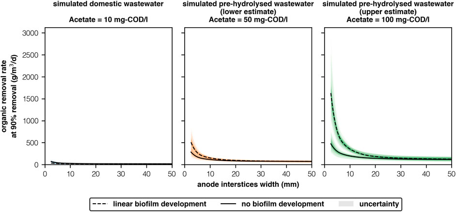
FIGURE 1. ORR at 90% substrate removal for simulated wastewaters with different acetate concentrations (10-100 mg-COD/l) and anode interstices widths (2.5–50 mm) [2 columns].

Pre-hydrolysing wastewater will allow for financially-competitive MECs provided anode interstices are sufficiently narrow and biofilms are well-developed. The highest ORR occurred when acetate concentrations were 100 mg-COD/l and interstices were 2.5 mm. Under “linear biofilm development,” ORR (1,630 ± 380g-COD/m³/d) surpassed targets for financial viability (800–1,400g-COD/m³/d) (Aiken et al., 2019). And, was more than double the ORR achieved when widths were twice as broad (765 ± 155g-COD/m³/d). Previously, acetate concentrations of 100mg/L have been achieved by hydrolysing domestic wastewater (Ligero et al., 2001)–though unreliably (20-100 mg-COD/l). ORR are highly sensitive to acetate concentrations (Figure 1). For a more conservative 50 mg-COD/l with an interstices width of 2.5 mm, ORR were 69% lower than achieved at 100 mg-COD/l (508 ± 126g-COD/m³/d, “linear biofilm development,” Figure 1). Accounting for additional substrate removal expected in the “real-world”–this may still be sufficient to achieve viability targets if costs are sufficiently low.

Hydrolysis alone is insufficient for MECs to be viable. Rather, it is the relationship between interstices width and acetate concentration that controls an MECs’ financial competitiveness. MECs can achieve significantly higher ORR when interstices are between 2.5 and 10 mm, under both development scenarios and at all acetate concentrations. Interestingly, this relationship is non-linear. When interstices are greater than 10 mm, interstices width had very little effect on ORR. When anodes were 20–50 mm apart ORR were low (117-185g-COD/m³/d, 100 mg-COD/l). Any successful reactor will therefore need to design anode chambers and treatment systems accordingly. MECs with narrower interstices perform best because organic removal rates (ORR) from biofilm activity are higher than from the bulk community, likely due to higher biofilm biomass concentrations, though we were unable to confirm this due to issues with equifinality. As interstices reduce, more organics are readily available for uptake from the biofilm.

The model failed to compute ORR for the “linear biofilm development” scenario when interstices were less than or equal to 2 mm as the model became unbounded, strongly suggesting that in these narrow chambers there was insufficient acetate to support a sufficiently large biofilm. This was also shown empirically by Chen et al. (2012), who observed MEC current production declining when interstices were less than 2.2 mm and not before. Therefore anodes that have narrower interstices may be limited. Previous pilot reactors have predominantly used “3 dimensional” anode structures such as carbon felt (Heidrich et al., 2013; Escapa et al., 2015; Baeza et al., 2017; Cotterill et al., 2017) and carbon brushes (Cusick et al., 2011). Both materials have high surface area, but also extremely narrow interstices (c.100 μm). The latter may explain why no pilot reactor to date has excelled. If so, novel materials will be needed to achieve suitably high performances.

High quality control during anode manufacturing is needed to ensure all interstices are sufficiently narrow (2.5 mm). However, narrower interstices ($<$10 mm) are likely to result in clogging when fed with “real” domestic wastewater due to the presence of suspended particles (Aelterman et al., 2008). If used for pre-treatment, up-flow hydrolysis reactors can retain some, but likely not all, suspended solids (SS). Further pre-treatment, such as screening, will be required to remove and dispose of SS, increasing cost. Wider interstices (10 mm) would mitigate this problem, but would significantly reduce ORR (78% lower). To facilitate sufficient mass transport in narrow interstices large MEC may require a modular design, increasing cost. Alternatively, convection may be increased, though an increase in turbulence could reduce biofilm size (Fink et al., 2016).

If biofilm development is poor then ORR will not reach targets. Poor biofilm development had the highest impact on ORR. The difference in ORR between the “no biofilm development” scenario (473 ± 141g-COD/m³/d, 2.5 mm, 100 mg-COD/l) and “linear biofilm development” scenario (1,630 ± 380g-COD/m³/d, 2.5 mm, 100 mg-COD/l) is highly significant. As biofilm development likely lies between our two projections, further empirical work will be needed to confirm the results from these, though we hope that these projections provide researchers and technologists with a floor and ceiling for MEC performance, in temperate conditions, with respect to acetate concentrations and interstices’ widths. Moreover, biofilms typically undergo growth and death cycles and further work will also be needed to investigate the risk of biofilm failure.

3.2 MEC Anode Chamber Design

Faster reactors are smaller reactors. The colonisable anode surface area needed to support sufficient biofilm development to treat a given flowrate is a function of the interstices width and the size of the reactor (Figure 2). Under “linear biofilm development,” when widths are broad ($>$12 mm) and concentrations are high, time taken to reach 90% substrate removal is longer. However, when widths are narrow ($<$12 mm) and concentrations are high, time taken to reach 90% substrate removal is shorter. Narrower interstices ($<$12 mm) therefore reduce both an MEC’s retention time, size and anode surface area when acetate concentrations are high (100 mg-COD/l).

FIGURE 2

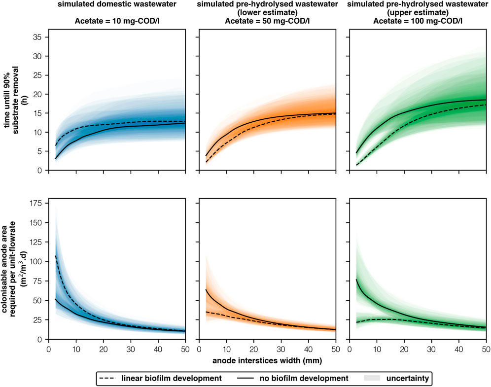
FIGURE 2. Time until 90% substrate removal and associated anode surface area requirements per unit-flowrate for effective treatment of simulated wastewaters with different acetate concentrations (10-100 mg-COD/l) and anode interstices widths (2.5–50 mm) [2 columns].

The fastest, and thus the smallest reactor (100 mg-COD/l, 2.5 mm, “linear biofilm development”) was predicted to achieve 90% removal of acetate in 1h18 ± 0h23 and will require 21.7 ± 6.4m²/m³.d to support “sufficient” biofilm biomass. If interstices are narrow but pre-hydrolysis is poor (50 mg-COD/l, 2.5mm, “linear biofilm development”) 90% removal will be marginally slower (2h06 ± 0h30) and larger anodes are needed to support a more diffuse biofilm (35.1 ± 8.4m²/m³.d). If anode quality control is poor (100 mg-COD/l, 5 mm, “linear biofilm development”) then removal will be significantly longer (2h49 ± 0h35)–though area requirements are only marginally higher (23.4 ± 4.9 m²/m³.d). Furthermore, if interstices are wide, to prevent blockages (100 mg-COD/l, 10 mm, “linear biofilm development”), then retention times will be significantly larger (6h05 ± 1h21), and increases in anode area are needed to treat the same flowrate (45.8 ± 8.7m²/m³.d). Most importantly, biofilms must be well developed and relatively stable. Poor biofilm development (100 mg-COD/l, 2.5 mm, “no biofilm development”) will require significant increases in both removal time (4h35 ± 1h16) and anode area (76.4 ± 21.0m²/m³.d).

If interstices are narrow ($<$10 mm) and acetate concentrations high (100 mg-COD/l), MECs could have significantly smaller HRT than typical for AS (5–14 h) (Stott, 2003). Therefore, an MEC would be retrofittable into aeration chambers, provided cathodes are small. However, this presupposes that most of the COD in the influent is converted into acetate or other quickly digested VFAs. Failing this, MECs will require longer retention times or cheaper post-treatments to “polish” effluent to standard. Moreover, removal times will likely vary with substrate concentrations and biofilms undergo growth and death cycles (Judd, 2013) and therefore larger anode areas are needed. Considering biofilm stability and applying a safety factor around 2–5x our ideal scenario, a rough conservative measure for anode area per flowrate could be 50–100 m²/m³.d, depending on the material, cost, prior testing and risk tolerance. Material surface area should only count towards area requirements if the surface is accessible and capable of supporting an electroactive biofilm. Materials with very high specific surface areas, such as activated carbon cannot have the majority of their surface counted, as the high surface area is predominantly in the form of a multitude of pores with small diameters ($<50\mu$m). The most suitable materials will be flat carbon surfaces that can be packed tightly together and porous carbon materials with pores greater than 2 mm. We challenge researchers and technologists to acquire or create new anodes that fit this requirement.

3.3 Standard Unit Cost

Reactors with densely packed anodes benefit from higher ORR and thus higher allowed capital costs (Aiken et al., 2019). Moreover, sufficient anode area requirements reduce when interstices are narrow and concentrations are high (2.5 mm, 100 mg-COD/l, “linear biofilm development” Figure 2). Consequently, allowable standard costs for MEC reactors (standardised/m²-anode) to break-even are significantly higher in our best scenario (2.5 mm, 100 mg-COD/l, “linear biofilm development,” Figure 3) due to this “double positive” effect. Standard costs to break-even were £16 ± 2/m², £21 ± 2/m² and £30 ± 4/m² for 5, 10 and 20 year time-frames, respectively. However, if biofilm development is poor (2.5 mm, 100 mg-COD/l, “no biofilm development”) standard costs are £1.60 ± 1.04/m², £2.40 ± 1.30/m² and £3.60 ± 2.00/m² for 5,10 and 20 years, respectively.

FIGURE 3

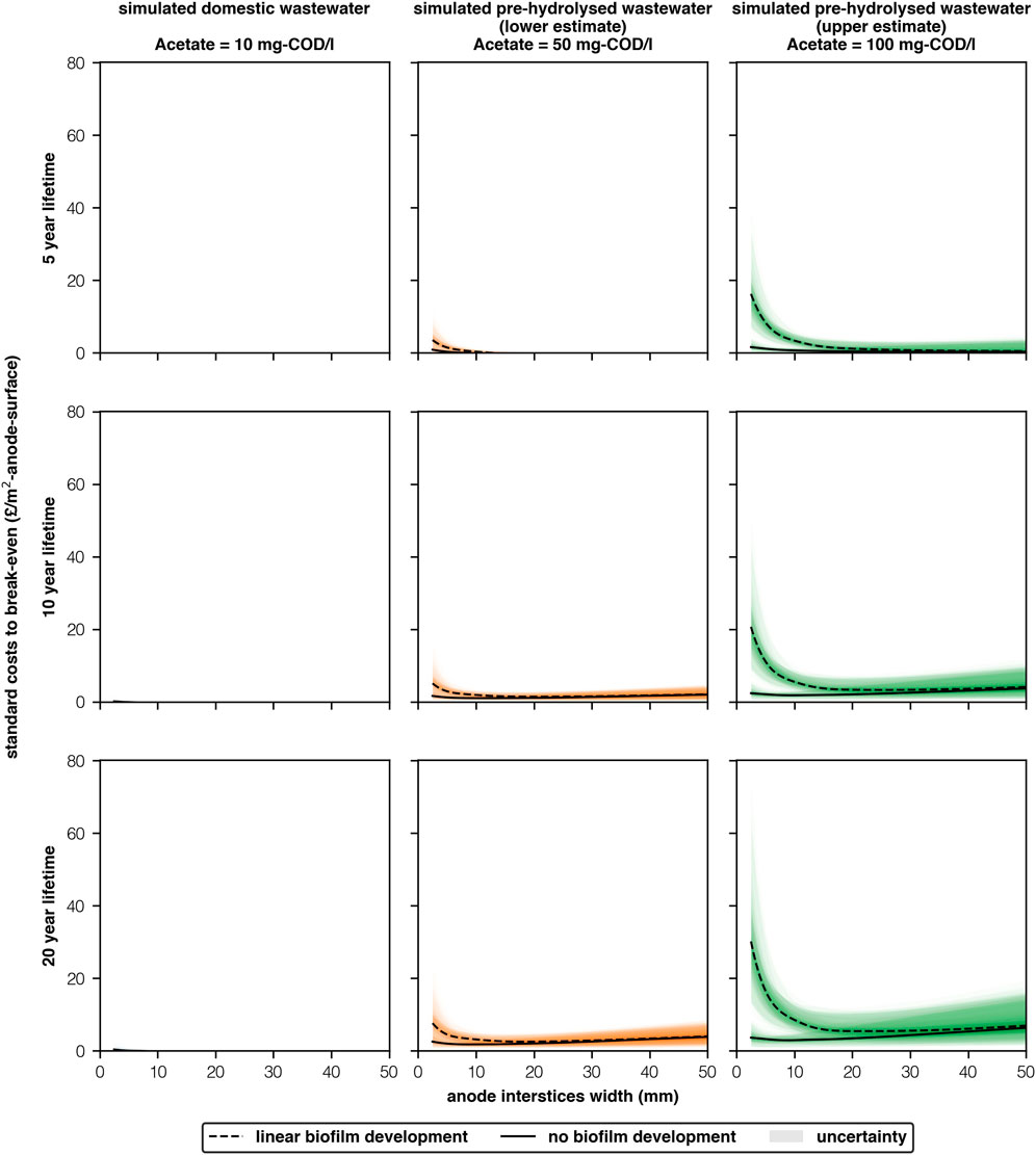
FIGURE 3. Allowable standard costs (/m²-anode) for MECs to break-even with AS treating simulated wastewaters with different acetate concentrations (10-100 mg-COD/l), anode interstices widths (2.5–50 mm) and service life-times (5–20 years) [2 columns].

Biofilm growth was the largest factor affecting standard costs (Figure 3). If biofilm development is close to the “linear biofilm development” scenario then allowable standard costs appear sufficiently high that future MEC technologists should be able to work with materials whose prices are within these bounds. However, if biofilm development is closer to the “no biofilm development” scenario It is unlikely that sufficiently cheap materials can be sourced: the cheapest material in a recent MEC pilot was the membrane (£1/m²-membrane, Rhinohide, Entek, United Kingdom) (Aiken et al., 2019).

In reality it is most likely that mean performance will be somewhere between the “linear biofilm development” and “no biofilm development” scenarios, and removal will not consistently meet standards (European Economic Community Council, 1991). Reducing material costs to around £5–10/m² would allow for some tolerance in development, whilst still retaining the possibility of being cost-effective in the long-term. Though, this will not protect against completely poor performance. Researchers and technologists will need to base any costs on their own reactor’s performance.

3.4 Biofilm Activity

ORR is higher with narrower interstices’ because biofilm activity is greater than bulk community activity (Figure 5). As interstices’ become narrower, the biofilm plays a larger role in substrate degradation as shown by the increase in coulombic efficiency (Figure 4). There is insufficient substrate available to replace that which is consumed by the biofilm. Maximum current density remains the same at narrower interstices but substrate and current both degrade faster (Figure 4). This was true of both scenarios, regardless of parameter uncertainty.

FIGURE 4

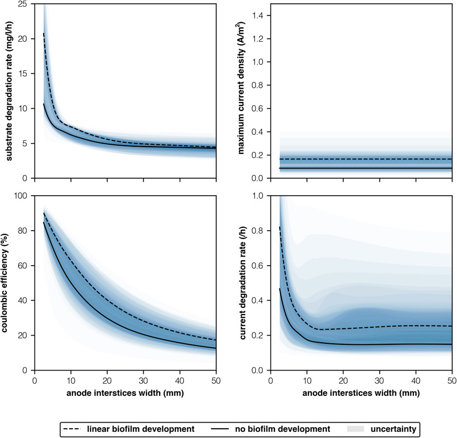
FIGURE 4. Model predictions with respect to anode interstices’ width (mm) at 50 mg-COD/l.

Our model assumes that biomass concentrations remain the same regardless of width. As current density is a function of the biofilm, we believe this serves as a proxy. Chen et al. (2012) observed that in an MFC fed with 20 mM of acetate (1,260 mg-COD/l) current densities declined when interstices’ widths were reduced below 2.2 mm and not before. At interstices widths of 2.2, 2.9 and 3.2 mm current densities were around 7.0A/m². Whilst at 1.4 mm current density reduced to 4.7 A/m². Chong et al. (2019) conducted a review of 71 papers and found that the greatest reduction in planar current densities occurred when pore sizes were <0.5 mm due to pH inhibition. This was further speculated as an important limiting factor by Logan et al. (2006). However, only 5 out of the 71 papers had anode interstices with widths >0.5 mm and broader chambers (>1 mm) were not considered.

We did not consider the impact of a reduced HRT on biofilm development. If all substrate is consumed in a short period of time reactors could be fed more frequently, and could hypothetically support a larger biofilm as more substrate would enter the biofilm. However, this would only further highlight our findings on the importance of the relationship between anode interstices’ width and cost-performance. We encourage experimentalists to investigate further.

3.5 Calibration

In multi-objective problems, there exist a set of optimal solutions that trade off between different objectives, known as the Pareto Front (Weicker and Weicker, 2003). Obtaining higher accuracies beyond this front is impossible as any improvement in one objective leads to a deterioration in one or more of the other objectives. The two best fitting schemes had a “mean accuracy” of 96.4% with starting acetate concentrations of 21.2 mg-COD/l and 39.4 mg-COD/l. The best fitting schemes for the remaining concentrations: 14.7 mg-COD/l, 16.4 mg-COD/l, 22.4 mg-COD/l and 35.4 mg-COD/l, had mean accuracies of 87.6%, 88.4% 94.6 and 86.9%, respectively. As the algorithm was not designed to map the whole parameter space, it is possible that better fitting parameters exist for these concentrations but that the fitness function was unable to select for them. However, as accuracy was measured against a particular concentration, a higher accuracy does not necessarily mean that the parameters of that run fit well with the other concentrations.

Moreover, empirical observations are themselves a model. Measurements were made using a combination of chemical and electronic signals that present information about an underlying reality but do not exactly map it. Uncertainties in empirical measurements mean that the lab results themselves cannot be entirely relied upon. Indeed, one of the starting concentrations (16.4 mg-COD/l) failed to find any combination of parameters that had outputs that were within all four of the observed ranges. This is likely because the feeding run at 16.4 mg-COD/l had a lower maximum current density and coulombic efficiency than the feeding run at 14.7 mg-COD/l, despite containing a higher starting acetate concentration and having a larger substrate degradation rate.

We present our results to demonstrate uncertainties resulting from parameter estimation of mean observations for microbial electrolysis cells with well-developed biofilms. Uncertainty increased as concentration increased. In the laboratory we fed our reactors with low acetate concentrations (10-50 mg-COD/l). As a result, the model was not constrained above these concentrations and as the concentration of acetate became greater than 50 mg-COD/l the predictions from the model were more uncertain due to uncertainties in the parameters (Figure 5). By uniformly randomising the starting concentrations for each iteration within each of the generations, the algorithm was only softly constrained by any one measurement. Permutations were assessed, each generation, based on their selective fit against any one of the concentrations and in the subsequent generation the parameters were rearranged and assessed against any other. If one concentration, or a group of concentrations, fit better than another, then the permutations that had poorer fit would be selected against, thus reducing overfitting. However, due to the stochastic nature of the algorithm, there still lies a small possibility, that a high accuracy measurement fits one of the starting concentrations very well but not the others. Therefore, observing the extrapolation results as probabilistic and viewing the median gives a more accurate picture of the “global” solution. Furthermore, rerunning the algorithm many times further reduces this possibility and the impact that random starting permutations, and combinations have on the final output. By looking at the top results for each starting concentration, rather than the most accurate solutions, we consider both the global solution and the uncertainties in parameter estimation.

FIGURE 5

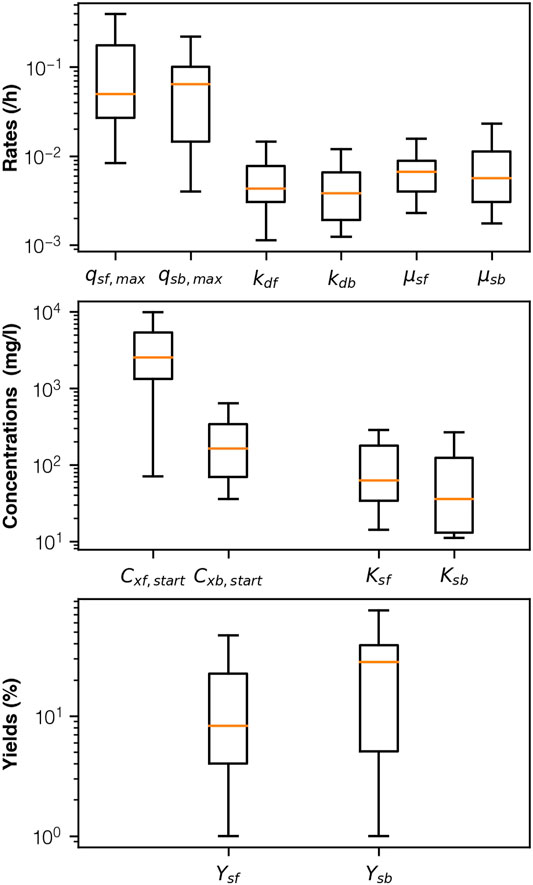
FIGURE 5. Box-plot description for “best fit” parameters following calibration. Largest difference between biofilm and bulk community observed for biomass concentration [1 column].

Parameter estimation was further confounded by issues with equifinality in some of the parameters. A notable example is that of maximum substrate degradation rate and biomass. The substrate degradation, which we calibrated for took the product of these parameters (Eq. 1) and neither was constrained by observation. Extrapolating to higher concentrations beyond 100 mg-COD/l showed a wider range of predicted substrate degradations and current densities. Yet, despite this solutions converged when interstices widths were narrower. Moreover the non-linear relationship between width and ORR held for all permutations regardless of whether the concentration of biomass increased or remained stable with changes in acetate concentration. This is because in order for the mechanics of the system to fit with observed current densities and substrate degradation rates microbial activity in the biofilm must have been higher than in the bulk liquid.

3.6 Validation

None of our observations particularly favoured either the “no growth” or “linear growth” scenarios when plotted against acetate concentration (Figure 6). Moreover, very few studies investigate electrogenic biofilm activity at low temperatures despite activity being a function of temperature, and those that do consider different substrates at much higher COD concentrations (Larrosa-Guerrero et al., 2010; Lu et al., 2012). In all likelihood performance lies somewhere between these two scenarios and we present these as a floor and a ceiling for MEC performance.

FIGURE 6

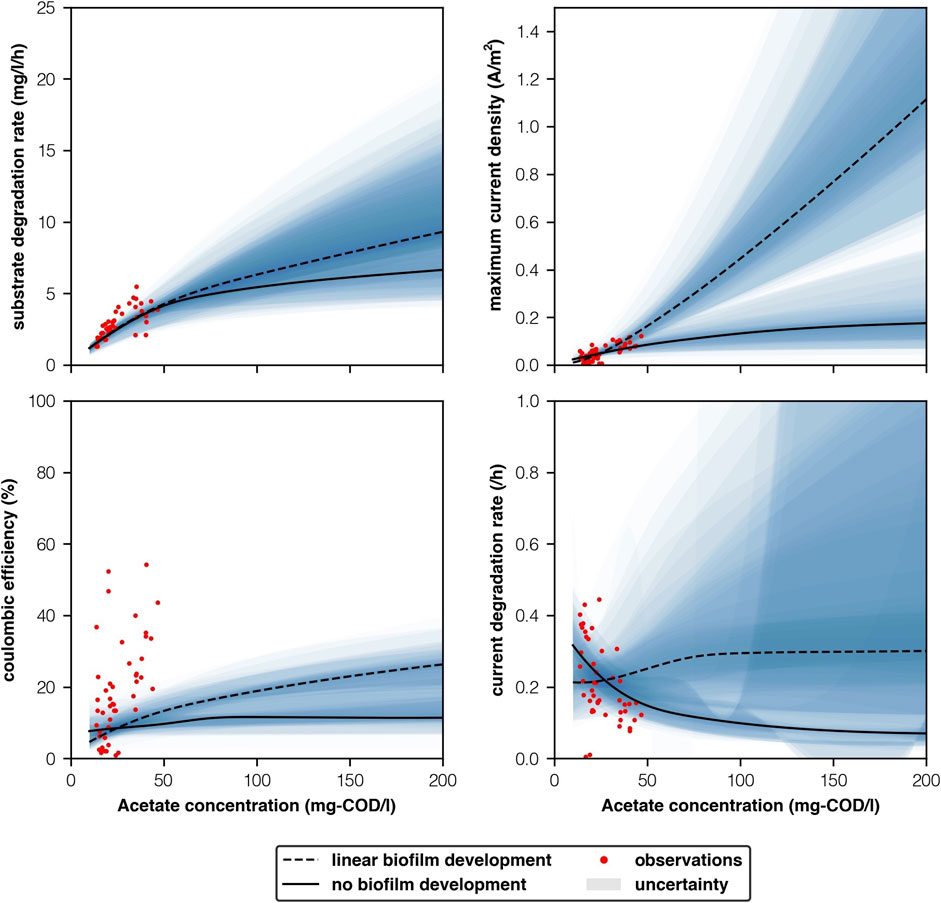
FIGURE 6. Empirically observed parameters vs model predictions with respect to acetate concentration (mg-COD/l).

Our model predicted substrate concentration well, between 10 and 50 mg-COD/l. Both scenarios predicted similar substrate degradation rates at these concentrations. Beyond 50 mg-COD/l the scenarios began to diverge. At 100 mg-COD/l the “linear biofilm development” predicted higher substrate degradation rates (6.3 ± 2.7g-COD/l.h vs 5.4 ± 2.9g-COD/l.h). Higher acetate concentrations showed that the “linear biofilm development” scenario continued to achieve higher substrate degradation rates. This is unlikely in reality as higher concentrations can have an inhibiting effect (Mateo et al., 2019). We therefore believe that the “linear growth” scenario over predicts substrate degradation rate when concentrations are high (>100 mg-COD/l) and interstices’ wide (>10 mm). Moreover, Zhao (2018) found that when reactors were acclimated with high acetate concentrations Geobacteraceae dominated (91% of anodic microbial community, qPCR). Thus, bulk community biomass concentrations may diminish as electrogenic organisms outcompete them for substrate.

Maximum current density is a function of the biofilm, whilst substrate degradation rate is a function of both the biofilm and bulk community. Therefore ORR at narrower interstices’ when the biofilm dominates is most affected by our prediction of maximum current density. Divergences in maximum current density between the two scenarios are stark (Figure 6). Observations for maximum current density had a linear relationship with acetate concentration, as was expected from observations. However, our observations appear to lie between the “no growth” and “linear growth” scenarios. Though there is far too much variability in measurements and too little difference between the scenarios at low concentrations to give credit one way or the other using these measurements. At 2.5 mm, 1,260 mg-COD/l, our “linear biofilm development” scenario (9.5 ± 12.9 A/m²) better agreed with Chen et al. (2012)’s observations of 7.0 A/m² than our ’no biofilm’ development scenario (0.2 ± 0.2 A/m2). However, uncertainties in our predictions were high relative to the median and this experiment was conducted at a higher temperature. Further work with low temperatures (10°C) and narrow anode interstices’ (c.2.5 mm) is needed.

Coulombic efficiency was not well mapped by changes in acetate concentration (Figure 6). In the lab we observed a large range of efficiencies at relatively small concentrations, which may mean that that the link between these phenomenon is either negligible or indirect. Current degradation rate’s relationship with acetate concentration appeared to be best mapped by the “no growth” scenario (Figure 6). However, the relationship between current degradation rate and acetate concentration is still unclear and is not well understood. Furthermore, the “no growth” scenario became somewhat unstable at acetate concentrations greater than 50 mg-COD/l. Whilst, the “linear growth scenario” remained stable and similarly mapped the centre of the data points we observed (Figure 6). Further study is needed before any conclusions on current degradation rate can be made.

4 Conclusion

Domestic wastewater contains too little acetate (10 mg-COD/l), in its typical form, for MECs to be a viable alternative to AS. ORR are higher when anode interstices are narrower because biofilm activity is greater than bulk community activity. The highest performing MECs are predicted to occur when interstices are sufficiently narrow (2.5 mm). Narrower interstices ($<$2.5 mm) may limit mass transport and thus reduce performance. We estimate that a commercially viable MEC design could be obtained when: standard costs for the new system are reduced to around £5–10/m²-anode - wastewater is pre-treated using hydrolysis to obtain a steady supply of acetate ($>$100 mg-COD/l) - and anode interstices’ widths (2.5 mm) are carefully controlled. Biofilms must relatively stable over an MEC’s operational and quality control must be of a high standard.

Data Availability Statement

The original contributions presented in the study are included in the article/Supplementary Material, further inquiries can be directed to the corresponding author.

Author Contributions

All authors conceived and designed the study. DA conducted the experiments, designed and built the models, analysed and interpreted the results and drafted the manuscript. All authors reviewed the results, revised the manuscript and approved the final version for publication.

Funding

The authors declare that this study received funding from the EPSRC and the Northumbrian Water Group (EP/L015412/1) through the STREAM Industrial Doctorate Centre, United Kingdom. The funder was not involved in the study design, collection, analysis, interpretation of data, the writing of this article or the decision to submit it for publication.

Conflict of Interest

The authors declare that the research was conducted in the absence of any commercial or financial relationships that could be construed as a potential conflict of interest.

Publisher’s Note

All claims expressed in this article are solely those of the authors and do not necessarily represent those of their affiliated organizations, or those of the publisher, the editors and the reviewers. Any product that may be evaluated in this article, or claim that may be made by its manufacturer, is not guaranteed or endorsed by the publisher.

Supplementary Material

The Supplementary Material for this article can be found online at: https://www.frontiersin.org/articles/10.3389/fceng.2021.796805/full#supplementary-material.

References

Aelterman, P., Versichele, M., Marzorati, M., Boon, N., and Verstraete, W. (2008). Loading Rate and External Resistance Control the Electricity Generation of Microbial Fuel Cells with Different Three-Dimensional Anodes. Bioresour. Technol. 99, 8895–8902. doi:10.1016/j.biortech.2008.04.061

PubMed Abstract | CrossRef Full Text | Google Scholar

[dataset] Aiken, D. C., Curtis, T. P., and Heidrich, E. S. (2019). Avenues to the Financial Viability of Microbial Electrolysis Cells [MEC] for Domestic Wastewater Treatment and Hydrogen Production. Int. J. Hydrogen Energ. 44, 2426–2434. doi:10.1016/j.ijhydene.2018.12.029

CrossRef Full Text | Google Scholar

Baeza, J. A., Martínez-Miró, À., Guerrero, J., Ruiz, Y., and Guisasola, A. (2017). Bioelectrochemical Hydrogen Production from Urban Wastewater on a Pilot Scale. J. Power Sourc. 356, 500–509. doi:10.1016/j.jpowsour.2017.02.087

CrossRef Full Text | Google Scholar

[Dataset] Business Electricity Prices (2016). Business and Commercial Electricity Prices. Available at: http://www.businesselectricityprices.org.uk/ (Accessed September 11, 2018).

Google Scholar

Chen, S., He, G., Liu, Q., Harnisch, F., Zhou, Y., Chen, Y., et al. (2012). Layered Corrugated Electrode Macrostructures Boost Microbial Bioelectrocatalysis. Energ. Environ. Sci. 5, 9769–9772. doi:10.1039/c2ee23344d

CrossRef Full Text | Google Scholar

Cheng, H., Cheng, D., Mao, J., Lu, T., and Hong, P.-Y. (2019). Identification and Characterization of Core Sludge and Biofilm Microbiota in Anaerobic Membrane Bioreactors. Environ. Int. 133, 105165. doi:10.1016/j.envint.2019.105165

PubMed Abstract | CrossRef Full Text | Google Scholar

Chong, P., Erable, B., and Bergel, A. (2019). Effect of Pore Size on the Current Produced by 3-dimensional Porous Microbial Anodes: A Critical Review. Bioresour. Technol. 289, 121641. doi:10.1016/j.biortech.2019.121641

PubMed Abstract | CrossRef Full Text | Google Scholar

Cotterill, S. E., Dolfing, J., Jones, C., Curtis, T. P., and Heidrich, E. S. (2017). Low Temperature Domestic Wastewater Treatment in a Microbial Electrolysis Cell with 1 m2Anodes: Towards System Scale-Up. Fuel Cells 17, 584–592. doi:10.1002/fuce.201700034

CrossRef Full Text | Google Scholar

Cusick, R. D., Bryan, B., Parker, D. S., Merrill, M. D., Mehanna, M., Kiely, P. D., et al. (2011). Performance of a Pilot-Scale Continuous Flow Microbial Electrolysis Cell Fed Winery Wastewater. Bioenergy and Biofuels 89, 2053–2063. doi:10.1007/s00253-011-3130-9

CrossRef Full Text | Google Scholar

Dhar, B. R., and Lee, H.-S. (2014). Evaluation of Limiting Factors for Current Density in Microbial Electrochemical Cells (MXCs) Treating Domestic Wastewater. Biotechnol. Rep. 4, 80–85. doi:10.1016/j.btre.2014.09.005

PubMed Abstract | CrossRef Full Text | Google Scholar

Escapa, A., Gómez, X., Tartakovsky, B., and Morán, A. (2012). Estimating Microbial Electrolysis Cell (MEC) Investment Costs in Wastewater Treatment Plants: Case Study. Int. J. Hydrogen Energ. 37, 18641–18653. doi:10.1016/j.ijhydene.2012.09.157

CrossRef Full Text | Google Scholar

Escapa, A., San-Martín, M. I., and Mateos, R. (2015). Scaling-up of Membraneless Microbial Electrolysis Cells (MECs) for Domestic Wastewater Treatment: Bottlenecks and Limitations. Bioresour. Technol. 180, 72–78. doi:10.1016/j.biortech.2014.12.096

PubMed Abstract | CrossRef Full Text | Google Scholar

Europa (2008). HyWAYS the European Hydrogen Roadmap Contract. SES6-502596. Tech. rep.

Google Scholar

European Economic Community Council (1991). 91/271/EEC of 21 May 1991 Concerning Urban Waste-Water Treatment. Tech. Rep. L.

Google Scholar

Fink, R., Oder, M., Rangus, D., Raspor, P., and Bohinc, K. (2016). Microbial Adhesion Capacity. Influence of Shear and Temperature Stress. Int. J. Environ. Health Res. 25, 656–669. doi:10.1080/09603123.2015.1007840

CrossRef Full Text | Google Scholar

Heidrich, E. S., Dolfing, J., Scott, K., Edwards, S. R., Jones, C., and Curtis, T. P. (2013). Production of Hydrogen from Domestic Wastewater in a Pilot-Scale Microbial Electrolysis Cell. Appl. Microbiol. Biotechnol. 97, 6979–6989. doi:10.1007/s00253-012-4456-7

PubMed Abstract | CrossRef Full Text | Google Scholar

Henze, M., and Comeau, Y. (2008). “Wastewater Characterization,” in Biological Wastewater Treatment: Principles, Modelling and Design (London, UK: IWA Publishing), 33–52.

Google Scholar

Huang, M.-H., Li, Y.-M., and Gu, G.-W. (2010). Chemical Composition of Organic Matters in Domestic Wastewater. Desalination 262, 36–42. doi:10.1016/j.desal.2010.05.037

CrossRef Full Text | Google Scholar

Judd, S. (2013). Watermaths. second edn. Bedfordshire, UK: Judd and Judd Ltd.

Google Scholar

Kolmos, H. J. J. (2012). Brock Biology of Microorganisms. 13th edn. San Francisco, CA: Benjamin-Cummings.

Google Scholar

Larrosa-Guerrero, A., Scott, K., Head, I. M., Mateo, F., Ginesta, A., and Godinez, C. (2010). Effect of Temperature on the Performance of Microbial Fuel Cells. Fuel 89, 3985–3994. doi:10.1016/j.fuel.2010.06.025

CrossRef Full Text | Google Scholar

Leaist, D. G., and Lyons, P. A. (1984). Diffusion in Dilute Aqueous Acetic Acid Solutions at 25°C. J. Solution Chem. 13, 77–85. doi:10.1007/BF00646041

CrossRef Full Text | Google Scholar

Ligero, P., Vega, A., and Soto, M. (2001). Pretreatment of Urban Wastewaters in a Hydrolytic Upflow Digester. Water SA 27, 399–404. doi:10.4314/wsa.v27i3.4984

CrossRef Full Text | Google Scholar

Logan, B. E., Hamelers, B., Rozendal, R., Schröder, U., Keller, J., Freguia, S., et al. (2006). Critical Review Microbial Fuel Cells: Methodology and Technology. Environ. Sci. Technol. 40, 5181–5192. doi:10.1021/es0605016

PubMed Abstract | CrossRef Full Text | Google Scholar

Logan, B. (2008). Microbial Fuel Cells. Hoboken, New Jersey, USA: John Wiley & Sons.

Google Scholar

Lu, L., Xing, D., Ren, N., and Logan, B. E. (2012). Syntrophic Interactions Drive the Hydrogen Production from Glucose at Low Temperature in Microbial Electrolysis Cells. Bioresour. Technol. 124, 68–76. doi:10.1016/j.biortech.2012.08.040

PubMed Abstract | CrossRef Full Text | Google Scholar

Mateo, S., Mascia, M., Fernandez-morales, F. J., Rodrigo, M. A., and Di Lorenzo, M. (2019). Assessing the Impact of Design Factors on the Performance of Two Miniature Microbial Fuel Cells. Electrochimica Acta 297, 297–306. doi:10.1016/j.electacta.2018.11.193

CrossRef Full Text | Google Scholar

Metcalf, E., Tchobanoglous, G., Burton, F. L., and Stensel, H. D. (2003). Wastewater Engineering: Treatment and Reuse. 4th ed. edn. New York, USA: McGraw-Hill.

Google Scholar

Rabaey, K., and Verstraete, W. (2005). Microbial Fuel Cells: Novel Biotechnology for Energy Generation. Trends Biotechnol. 23, 291–298. doi:10.1016/j.tibtech.2005.04.008

PubMed Abstract | CrossRef Full Text | Google Scholar

Rozendal, R. A., Hamelers, H. V. M., Rabaey, K., Keller, J., and Buisman, C. J. N. (2008). Towards Practical Implementation of Bioelectrochemical Wastewater Treatment. Trends Biotechnol. 26, 450–459. doi:10.1016/j.tibtech.2008.04.008

PubMed Abstract | CrossRef Full Text | Google Scholar

Shi, C. Y. (2011). Mass Flow and Energy Efficiency of Municipal Wastewater Treatment Plants. London, UK: IWA Publishing.

Google Scholar

Sleutels, T. H. J. A., Darus, L., Hamelers, H. V. M., and Buisman, C. J. N. (2011). Effect of Operational Parameters on Coulombic Efficiency in Bioelectrochemical Systems. Bioresour. Technol. 102, 11172–11176. doi:10.1016/j.biortech.2011.09.078

PubMed Abstract | CrossRef Full Text | Google Scholar

Sleutels, T. H. J. A., Ter Heijne, A., Buisman, C. J. N., and Hamelers, H. V. M. (2012). Bioelectrochemical Systems: An Outlook for Practical Applications. ChemSusChem 5, 1012–1019. doi:10.1002/cssc.201100732

PubMed Abstract | CrossRef Full Text | Google Scholar

Speers, A. M., and Reguera, G. (2012). Electron Donors Supporting Growth and Electroactivity of Geobacter Sulfurreducens Anode Biofilms. Appl. Environ. Microbiol. 78, 437–444. doi:10.1128/AEM.06782-11

PubMed Abstract | CrossRef Full Text | Google Scholar

Stanbury, P. F., Whitaker, A., and Hall, S. J. (2017). “Chapter 11 - Effluent Treatment,” in Principles of Fermentation Technology. Third Edition (Oxford, UK: Butterworth-Heinemann), 687–723. doi:10.1016/B978-0-08-099953-1.00011-9

CrossRef Full Text | Google Scholar

Stott, R. (2003). “Fate and Behaviour of Parasites in Wastewater Treatment Systems,” in Handbook of Water and Wastewater Microbiology. Editors D. Mara, and N. Horan (Cambridge, Massacusetts, USA: Academic Press), 1–832. doi:10.1016/b978-012470100-7/50032-7

CrossRef Full Text | Google Scholar

Velasquez-Orta, S. B., Yu, E., Katuri, K. P., Head, I. M., Curtis, T. P., and Scott, K. (2011). Evaluation of Hydrolysis and Fermentation Rates in Microbial Fuel Cells. Appl. Microbiol. Biotechnol. 90, 789–798. doi:10.1007/s00253-011-3126-5

PubMed Abstract | CrossRef Full Text | Google Scholar

Weicker, K., and Weicker, N. (2003). Basic Principles for Understanding Evolutionary Algorithms. Fundamenta Informaticae 55, 387–403.

Google Scholar

Xia, C., Zhang, D., Pedrycz, W., Zhu, Y., and Guo, Y. (2018). Models for Microbial Fuel Cells: A Critical Review. J. Power Sourc. 373, 119–131. doi:10.1016/j.jpowsour.2017.11.001

CrossRef Full Text | Google Scholar

Xin, X., He, J., Li, L., and Qiu, W. (2018). Enzymes Catalyzing Pre-Hydrolysis Facilitated the Anaerobic Fermentation of Waste Activated Sludge with Acidogenic and Microbiological Perspectives. Bioresour. Technol. 250, 69–78. doi:10.1016/j.biortech.2017.09.211

PubMed Abstract | CrossRef Full Text | Google Scholar

Zhao, F. (2018). The Effect of Complex Feed on Bioelectrochemical Systems (BESs) Performance. Ph.D. thesis. Newcastle-upon-Tyne, United Kingdom: Newcastle University.

Google Scholar

Nomenclature

(anode) interstices refers to the space between opposing anodes’ surfaces

standard unit cost material cost standardised to anode surface area

m²/m³.d colonisable anode surface area (m²) needed to support sufficient biofilm development to treat a given flowrate m³/d

AS activated sludge treatment

BES bio-electrochemical system

COD chemical oxygen demand

MEC microbial electrolysis cell

ORR organic removal rate

OLR organic loading rate