In Silico Prediction of Food Properties: A Multiscale Perspective

Several open software packages have popularized modeling and simulation strategies at the food product scale. Food processing and key digestion steps can be described in 3D using the principles of continuum mechanics. However, compared to other branches of engineering, the necessary transport, mechanical, chemical, and thermodynamic properties have been insufficiently tabulated and documented. Natural variability, accented by food evolution during processing and deconstruction, requires considering composition and structure-dependent properties. This review presents practical approaches where the premises for modeling and simulation start at a so-called “microscopic” scale where constituents or phase properties are known. The concept of microscopic or ground scale is shown to be very flexible from atoms to cellular structures. Zooming in on spatial details tends to increase the overall cost of simulations and the integration over food regions or time scales. The independence of scales facilitates the reuse of calculations and makes multiscale modeling capable of meeting food manufacturing needs. On one hand, new image-modeling strategies without equations or meshes are emerging. On the other hand, complex notions such as compositional effects, multiphase organization, and non-equilibrium thermodynamics are naturally incorporated in models without linearization or simplifications. Multiscale method’s applicability to hierarchically predict food properties is discussed with comprehensive examples relevant to food science, engineering and packaging. Entropy-driven properties such as transport and sorption are emphasized to illustrate how microscopic details bring new degrees of freedom to explore food-specific concepts such as safety, bioavailability, shelf-life and food formulation. Routes for performing spatial and temporal homogenization with and without chemical details are developed. Creating a community sharing computational codes, force fields, and generic food structures is the next step and should be encouraged. This paper provides a framework for the transfer of results from other fields and the development of methods specific to the food domain.

1 Introduction

Food engineering and modeling tend to be more difficult than in other areas as foodstuffs are inherently complex objects; biological processes initially define their organizations, structures, and compositions. They evolve rapidly during harvesting, transportation, and distribution. Food processing profoundly changes all the properties of food: composition, structure, physical states of the constituents, degradation, and production of new chemical compounds (Datta, 2016). In other words, successful modeling should capture the evolution of the physicochemical properties with the degree of processing but also the effects of the initial biological variability and of supply chain fluctuations. Storage, preservation, final preparation and digestion of processed foods also profoundly alter these properties (Bornhorst et al., 2016). Modeling in food addresses usually only one part of the complexity: only the evolution of an “averaged” food product is sought and not the variability between food products. Thermodynamic, transport and mechanical properties are therefore “averaged” over a representative structure, composition, and assumed constant or dependent on macroscale state variables (e.g., temperature, water content, etc.). With the rapid progress in modeling and simulation in other engineering disciplines, including materials, polymer science, and soft matter, this chapter argues that the implicit paradigm of averaging any aspect of food transformation may be challenged in the future. The lack of extensive and freely accessible “mechanistic” food properties databases motivated the quest for alternatives to classical modeling (Nesvadba et al., 2004). When they exist, they do not consider compositional and structure effects essential to processed foods characteristics. Moreover, simulating flows, transfer, reactions, creation of structures and their mechanical properties in realistic conditions remains beyond the reach of conventional approaches without adequate parameterization on real-life food products (Roos et al., 2016).

Directly calculating physicochemical properties of foods from pure phase data or atomistic structures paves the way to the direct simulation (from first principles) of their processing and preservation regardless of the food or its process. In this new perspective, the incomplete macroscale model in food is supplemented by an explicitly given microscopic model. Such a framework differs from earlier semi-empirical models tabulated in Ref. (Gulati and Datta, 2013). This article reviews a selection of techniques enabling the emergence of macroscopic behaviors from the knowledge of structures or molecules and their potential applications in food engineering. Indeed, the popularization of high-throughput measurement techniques encourages the development of modeling techniques capable of using directly as inputs 3D images from X-ray microcomputed tomography, laser-scanning confocal microscopy in UV, visible and midinfrared ranges Raman confocal microscopy). Ideally, the approaches need to be sufficiently robust and tailored to accommodate various strategies (fully or partially in silico) to replace food missing properties and incorporate chemical and structural food characteristics. The growing development of equation-free multiscale computation (Kevrekidis and Samaey, 2009), along with the widespread use of parallel and cloud computing, makes the passthrough to the scale where the decision is taken possibly without requiring an explicit macroscopic-level step. “Food system analysis” at any step of its transformation, storage, oral processing and digestion may nourish innovation in food but also reaches external communities, including medical communities, industry and authorities. Linked decisions across the scales with arbitrary levels of entanglement (Gear et al., 2003) could be used to evaluate the impact of existing or future practices.

The manuscript borrows several concepts and techniques that we have developed to fill in the gaps in continuum numerical approaches, and more generally, to introduce chemical information, which does not fit well in evolutive equations, governed essentially by conservation equations. From a thermodynamic point of view, we address in this paper problems which are entropy-driven and therefore not directly related to heat transfer or mechanical work. The vantage point adopted in the proposed computational framework suggests that two multiscale problems coexist: spatial and temporal. Abundant literature describes the first one. It is approached from the perspective of mathematical homogenization and applied to the prediction of diffusion coefficients. This technique should not be confused with techniques for averaging over volume elements. It does not focus on the observation scale to define heterogeneities but instead defines a very large equivalent medium in which local variations become negligible. The mathematical tool is asymptotic analysis. The same concept is required to predict temporal evolutions at the food scale from scales close to the vibration of atoms or molecules. The coherent macroscopic behavior emerges from the interactions of microscopic agents (solutes, macromolecules, cells). Therefore, spatial and temporal microscopic details are not smoothed out but rather integrated up to the scale of the food, usually using a procedural computing approach. The feasibility of combining chemical-level, microscopic-level and food-level is illustrated in the interactions between the food and its packaging. The chosen methodologies have sufficiently low computational cost to operate in loops and support food production problem-solving: e.g., resource and waste minimization, valorization by-products, safety, security and health issues (Bazilian et al., 2011). But what are the challenges and opportunities of modeling across scales?

1.1 The Scale Problem

It is tempting to think that all scales can be modeled continuously from atoms to the cycle of production, distribution, and consumption of food by a population of consumers. The grounds why this is not possible in a classical sense are illustrated in Figure 1 regarding the farthest scales from the observer (human scale): either in the direction of atoms or on the scale of a sufficiently large system (including more than one single food).

FIGURE 1

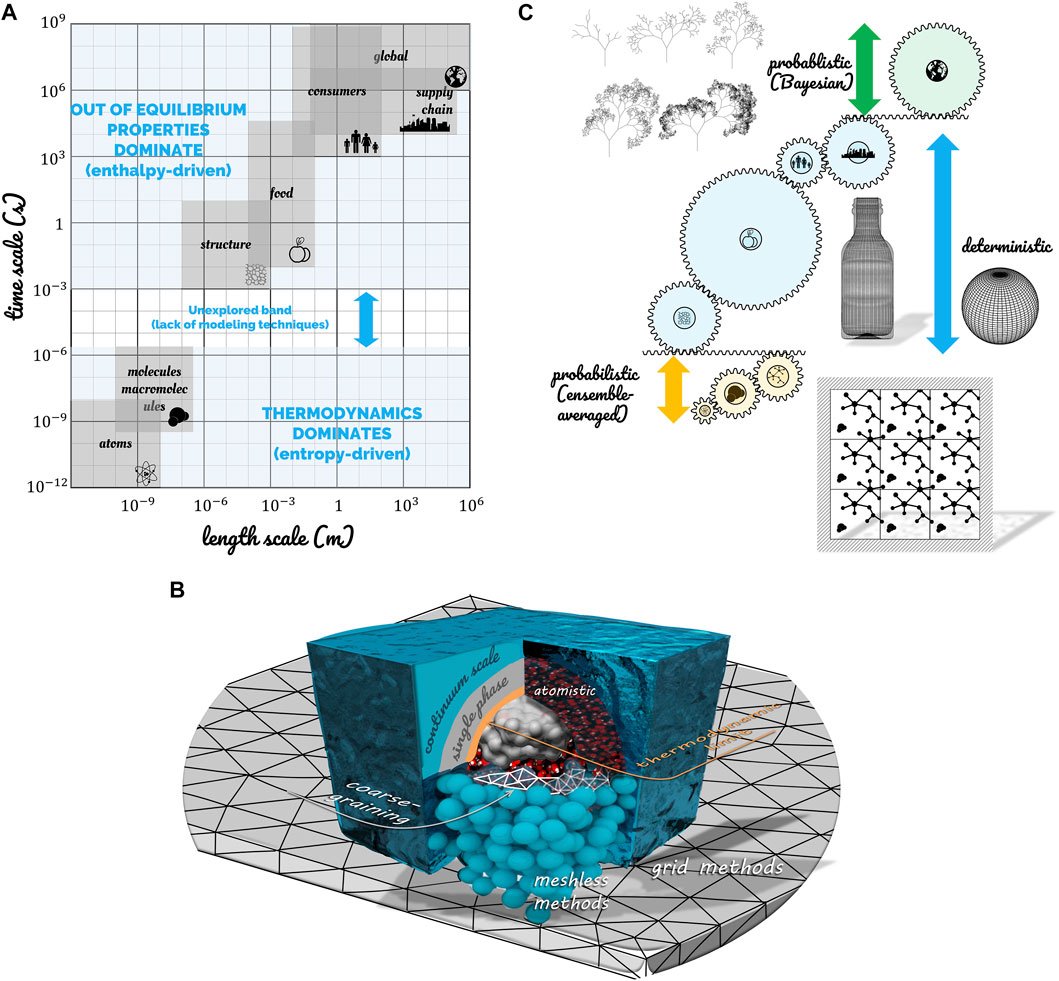
FIGURE 1. (A) Spanning of spatial and timescales associated with foods and identification of the time scale gap between thermodynamically controlled phenomena and out-of-equilibrium evolution of macroscopic systems. (B) Illustrations of techniques to simulate the phenomena on both sides of the thermodynamic limit (TL): grid and meshless ones above TL, atomistic or coarse-grained below TL. (C) Strategies of simulation across the scales.

At the finest scale, there are more molecules/entities in a 1 L water bottle (55.6 moles, i.e., 3.3 × 10²⁵ molecules; i.e., 10²⁶ atoms) than stars/entities in the observable universe [from 10²² to 10²⁴ according to the European Space Agency (ESA, n.d.)]. The most extensive simulation of a biophysical system at the atomic scale on an exascale supercomputer (130,000 cores) included only 10⁹ atoms/entities (Jung et al., 2019). If it were water, a cube of 215 nm side would contain this number of atoms. A water cube of 42 nm edge would require a more reasonable power of 1,000 cores. These volumes are insufficient to represent any food transformation (freezing/thawing, cooking, flow in a pipe), but they are sufficient to access fundamental properties at the nanometric scale. For example, the coalescence of two drops of 58.5 nm in diameter has been recently simulated at the atomic scale (Perumanath et al., 2019). The role of thermal fluctuations in the construction of a common liquid-gas interface has been demonstrated. This example illustrates three critical properties:

• Structural chemical information can only be maintained on scales commensurable with molecules and segments of polymers; beyond, structural and chemical information will have to be encoded using the principles of thermodynamics and mechanics on a larger scale.

• Statistical physics or mechanics can describe phenomena below the thermodynamic limit (TL), that is, when thermal fluctuations are significant. TL is much larger than molecules and also applies to colloidal systems (Frenkel, 2014).

• The union of systems smaller than TL does not allow the reconstruction of a macroscopic system by sampling. The property of additivity or extensivity is recovered only beyond TL.

There are no absolute rules to define the critical length scale for TL; TL tends to be longer in the presence of long-range forces or for systems with large surface-to-volume ratios in monophasic systems (Sheehan and Gross, 2006; Frenkel, 2014). In emulsions, foams, and suspensions, TL is much larger and reaches few micrometers.

The continuum scale (CS) lies between TL and an upper limit called “large scale” (LS). The “single-scale” approach is associated with finite-element and finite volume techniques. At these scales, there is no need to assemble forces on discrete systems and to assess the concept of thermodynamic and mechanic equilibrium locally. Statistical formulations are cast in conservation equations and resolved generically with the machinery of differential and integral calculus. Therefore, the food properties and driving forces are effective and capture most of the microscopic details in one single formulation. The properties are allowed to vary either with position, time, and intensive variables such as temperature, pressure, or local concentrations. The effective porous medium formulation describes well the effective heat transfer properties in heterogeneous food products such as dry foods. However, it is less efficient in deriving transport and mechanical properties as it does not consider phases spatial arrangement and morphology (Datta, 2007). Similarly, the corresponding driving forces (e.g., osmotic or swelling pressures) are well described for systems with low TL values (i.e., random mixtures of molecules). However, they may be more difficult to derive for systems presenting an organization at nanoscale or memory effects (i.e., dislocation, plasticity, glassy state) (Lucarini et al., 2020). Two examples easily illustrate the loss of details of the continuum approach at the food scale. The fracture of dry foods (e.g., chips) or rehydration of dry foods (e.g., cereals) will be described at continuum scale from the classical macro-strain without considering the anisotropic “micro strain” in cell walls and the effect of drying on the rigidity of cell walls. Similar microscopic effects occur when a native starch suspension is heated in a heat exchanger (Plana-Fattori et al., 2016). Gelatinization and swelling of starch granules will modify the viscosity locally and finally at a much larger scale. Microscopic gradients persist when two components with different viscosities are thermomixed such as during chocolate conching (Greiner et al., 2014).

Complex food simulators can be assembled from low-level mechanistic components for one particular food product. The concept of “large-scale” (LS) occurs when the same model is used for a broader range of food products. Its strict definition is more elusive and would correspond to situations where the underlying assumptions of at least one constitutive model cease to be verified. This model can be involved in either the prediction of effective properties or driving forces. The reasons could be: the raw biological materials are different (different variety, maturity, different tissues), the morphologies are different (different distributions for dispersed systems), the properties of the continuous phase are different (e.g., the addition of a thickening agent, fat replacers), different pretreatments (higher shrinkage, compaction), aging effects, etc.

1.2 Continuum vs. Discrete Descriptions

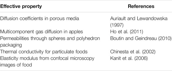
The core of this article is to highlight the different strategies to derive properties for food considered not as a uniform rigid body but as a soft matter organized at different scales. The choice of considering a discrete collection of interacting entities (molecules, phases) or an equivalent homogeneous continuum depends not only on the problem and the choice of the end-user but also on whether the chemical information needs to be considered explicitly or not. At this point, it is essential to note that no measurement is required for none of these methods beyond some information on the food composition and the spatial organization of phases herein. Counterintuitively, asymptotic analysis linking microscopic descriptions and standard mathematical formulation in simulation software (Comsol Multiphysics, OpenFoam, Fluent) are more abstract and require a minimum mathematical background. Conversely, particle methods used below TL (e.g., molecular or coarse-grained approaches) or above TL (Lagrangian descriptions) are more flexible and look more physical in particular to describe surface effects (coalescence, wetting, capillarity, adsorption, adhesion). The article presents both approaches, and both are sources of unavoidable errors. Replacing measured properties by computed properties (see calculable properties in Table 1) requires rigorous constructions and proper validation. The present article illustrates both methodologies when the sought property (transport coefficient, thermodynamic property) is:

• either a scalar or a symmetric tensor (anisotropic diffusion without no drift);

• either defined as a unique value or as a distribution of values.

TABLE 1

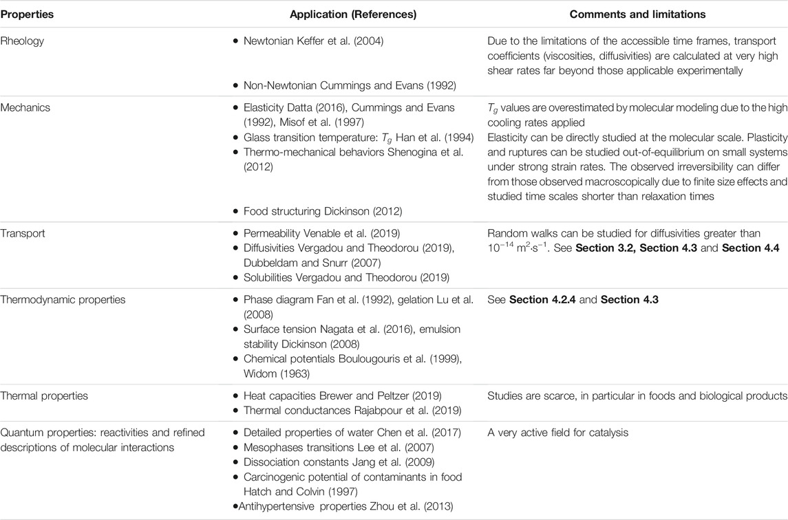
TABLE 1. List of input data in continuum mechanics model which can be predicted in silico from molecular and atomistic descriptions.

1.3 Problems in Food that Could be Resolved by Modeling at Multiple Scales

The concepts of modeling across the scales are still emerging in food, and the examples covering from molecular to very large scales are scarce in the literature. The authors developed experience in the field initially from molecules (Vitrac et al., 2006; Durand et al., 2010; Gillet et al., 2010; Vitrac and Gillet, 2010) to consumer exposure (Vitrac et al., 2007; Vitrac and Leblanc, 2007) with the intent of encouraging the industry and authorities to use high throughput predictive techniques for compliance testing and risk assessment. From our experience, the main obstacles to the generalization of large-scale modeling in food applications are:

- the lack of case studies showing how to combine deterministic and non-deterministic modeling in food engineering curriculum;

- the lack of a computational framework to combine tools obtained with different approaches (statistical physics, deterministic, stochastic);

- the difficulty to separate the phenomena occurring at different scales;

- the resistance of some practitioners and professionals who think that food cannot be reduced to algorithms.

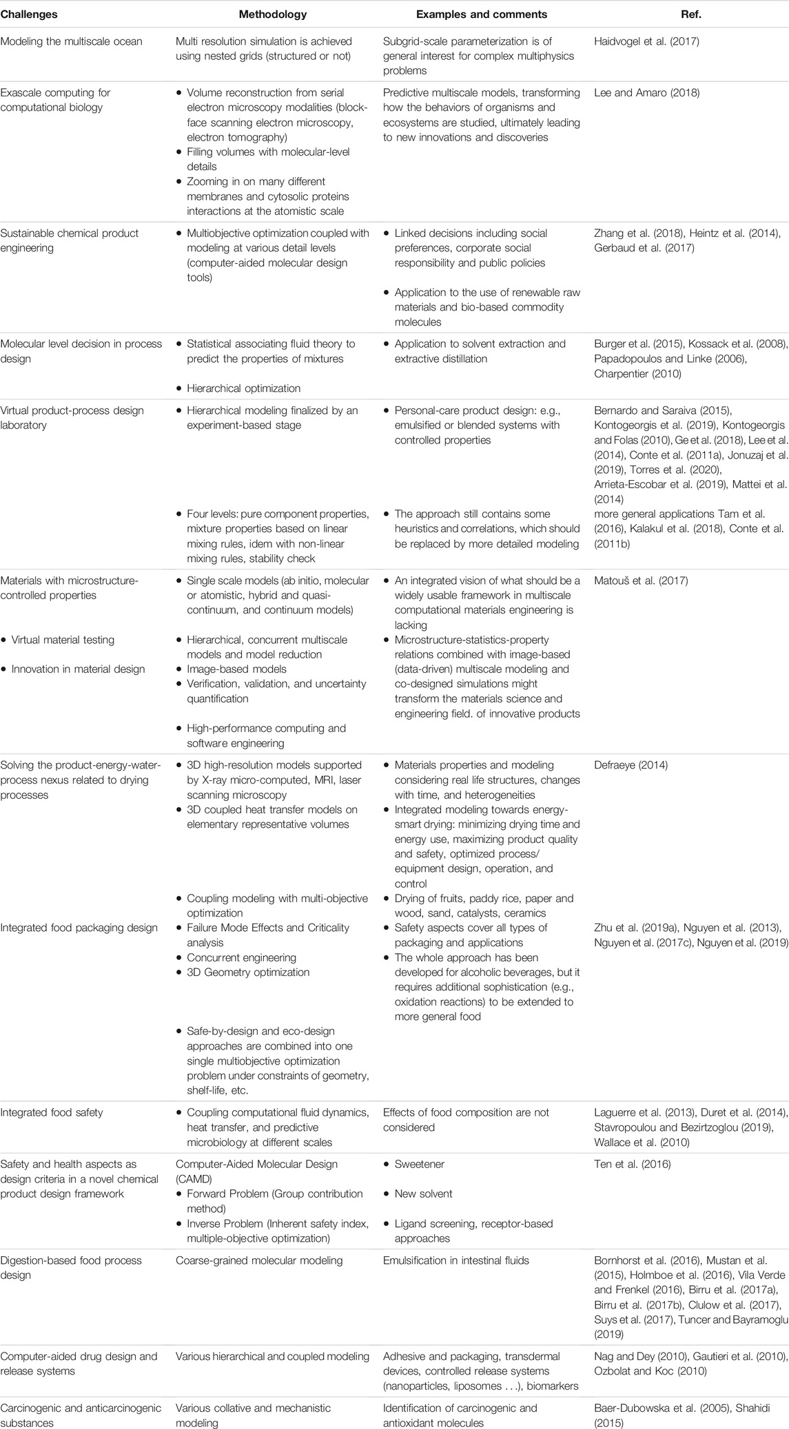
In related areas of food engineering, we argue that “modeling across the scales” has already produced very encouraging and competitive results. Table 2 lists the technological and societal challenges identified in the literature, which can be considered resolved or in the process of being resolved. The list is not exhaustive and indicates the dynamics of this theme for the coming decade. It is important to note that the most crucial point is not so much the multiscale modeling itself but the ability to reverse engineer the property being studied. The problem is no longer: “which property I need to supply to my model, but what does the model tell me about the property that could achieve the desired effect.” The introduction of the chemical and biochemical information allows tackling formulation and shelf-life determination problems from a mathematical point of view without the constraint of available raw materials or technologies. Food design becomes then a virtual activity supported by reusable libraries of self-similar problems. The chosen solution could be refined without extra costs for specific markets and consumers. Predictive property modeling methods are well documented in the literature but have not been implemented in the multiphysics software used by the food science and food engineering community.

TABLE 2

TABLE 2. Inspirational challenges of holistic modeling across the scales.

2 The Problem of Spatial Homogenization

Spatial homogenization is essential for modeling from 2D and 3D images. This section describes the general principles of spatial homogenization, as shown in Figure 2. The approach is applied to transform heterogeneous structures into effective media, whose properties can be encoded into commercial simulation software. Homogenization theory was elaborated in the 70s and 80s for composite materials; its application to structured foods (solid and semi-solid) is a natural extension. Classical homogenization is preferred to alternative approaches as it has received more formal proofs than other methods such as volume averaging and does not suffer complex entropy constraints for closure, such as the hybrid mixture theory (Battiato et al., 2019).

FIGURE 2

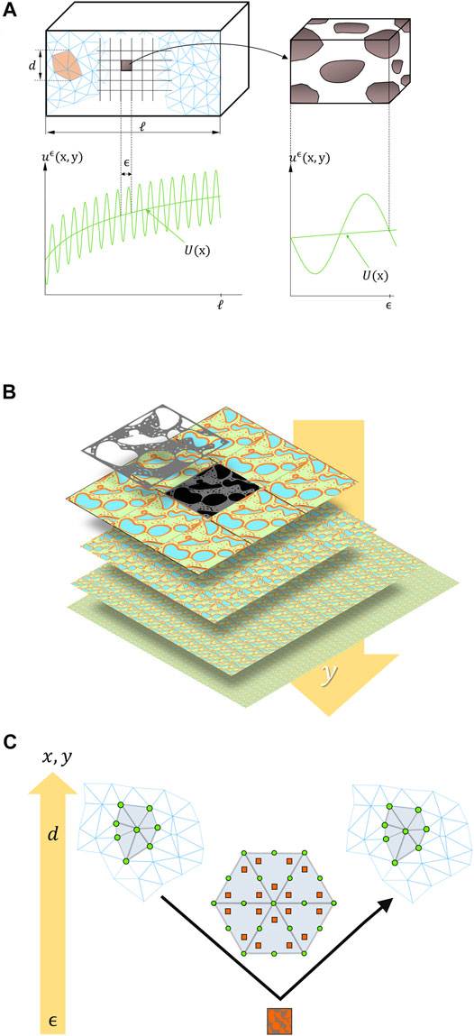
FIGURE 2. (A,B) Principles of homogenization of scale y at scale x: illustration of microscopic fluctuations of the local scalar $u^{\mathrm{ϵ}}\left(x,y\right)$ and its low-frequency approximation $U\left(x\right)$; example of periodic structure at several resolutions/scales. (C) Principles of the quadrature on a triangular mesh based on local microscopic values calculated on square microcells (orange). Circles show interpolation nodes.

2.1 General Formulation

Homogenization (time- or spatial-) aims to calculate effective properties for processes spanning over several time scales (e.g., combing rare events along with fast evolutions) or over heterogeneous structures. Any spatial-homogenization problem (not time-dependent) along the dimensionless coordinate $x$ (so-called slow variable) is recast as:

$L\left(x,y=\frac{x}{\mathrm{ϵ}}\right)u^{\mathrm{ϵ}}\left(x\right)=f\left(x\right)\mathrm{for}x\in \mathrm{\Omega }\subset R^n,(1)$

where $L\left(\right)$ is a differential operator (linear or not) and $y$ is the fast variable (fine-scale mapping) inducing the local fluctuations of the property. $u^{\mathrm{ϵ}}$ is the field (e.g., concentration, strain, temperature) calculated at the scale of the microstructure, so-called microscale. $\mathrm{ϵ}=\frac{d}{\ell }$ represents the ratio between the microscale $d$ and the macroscale $\ell$ (see Figure 2A).

Invoking Eq. 1 on the entire macroscale domain can be particularly expensive (typically $O^{-n}$ or more) and possibly not achievable for very small scales $\mathrm{ϵ}\ll \mathrm{1}$ or when the properties need to be updated regularly. The cost is usually reduced by assuming a separation of scales between the microscopic details and the macroscale domain simulated $\left(\mathrm{ϵ}\ll 1\right)$. It implies that beyond a critical scale ${\mathrm{ϵ}}_c$, $u^{\mathrm{ϵ}}$ converges to the macroscale solution $U$, which can be calculated at a much lower cost by solving the homogenized version of Eq. 1:

$\overline{L}\left(x\right)U\left(x\right)=f\left(x\right).(2)$

Finding an explicit homogenized equation $\overline{L}\left(x\right)$ from microscopic details may be a difficult mathematical problem and requires an adequate closure problem. Such equation exists as soon as $y\gg \frac{{\mathrm{ϵ}}_{\mathit{c}}}{\mathrm{ϵ}}$ (see Figure 2B) and is associated with effective properties, whose meaning is similar in various physical problems, but whose values reflect different microstructures and underlying phenomena, such as transport on distances smaller than the mean-free-path of molecules or transports controlled by rare events (e.g., trapping, surface adsorption, interactions with macromolecules). Many software packages can evaluate $U\left(x\right)$ using finite differences, finite volumes, finite elements, or higher-order spectral techniques based on proper property values. It is worth noticing that the volume source/sink term $f\left(x\right)$ appearing on the right-hand side of Eqs 1, 2 is assumed to be macroscopically imposed and, therefore, not subjected to microscopic fluctuations. Otherwise, the homogenization procedure cannot converge to a unique solution.

2.2 Identification of Homogenized Properties When Microscopic and Macroscopic Scales are Separable

2.2.1 Principles

The microscopic quantities $a^{\mathrm{ϵ}}\left(x,y=\frac{x}{\mathrm{ϵ}}\right)$ (static) or $a^{\mathrm{ϵ}}\left(x,y=\frac{x}{\mathrm{ϵ}},t\right)$ (dynamic) may be diffusivities (this example), permeabilities, elasticity moduli, reaction rate constants, etc. They converge to the effective properties when $y\gg 1$. It is worth noticing that homogenization does not aim at averaging the microscopic quantity $a^{\mathrm{ϵ}}\left(x\right)$, but the underlying conservation laws instead. By considering transport phenomena and due to the intertwining with other microscopic phenomena such as ad/absorption, $a^{\mathrm{ϵ}}\left(x\right)$ should only be envisioned as the property relating the microscale flux $j^{\mathrm{ϵ}}\left(x,t\right)=a^{\mathrm{ϵ}}\left(x\right)\nabla u^{\mathrm{ϵ}}\left(x,t\right)$ with the microscale driving force $\nabla u^{\mathrm{ϵ}}\left(x,t\right)$.

The corresponding microscopic advection-diffusion problem reads:

$\frac{\partial u^{\mathrm{ϵ}}\left(x,y,t\right)}{\partial t}+\nabla \cdot \left[b\left(\frac{x}{\mathrm{ϵ}}\right)u^{\mathrm{ϵ}}\left(x,y,t\right)\right]=\nabla \cdot \left[a^{\mathrm{ϵ}}\left(\frac{x}{\mathrm{ϵ}}\right)\nabla u^{\mathrm{ϵ}}\left(x,y,t\right)\right]-f\left(x\right).(3)$

By assuming that $a$ and $b$ vary smoothly over a periodic cell (of volume $V$) larger than ${\mathrm{ϵ}}_c$, Eq. 3 homogenizes as:

$\frac{\partial U\left(x\right)}{\partial t}+\nabla \cdot \left[\overline{b}\left(x\right)U\left(x\right)\right]=\nabla \cdot \left[\mathbf{A}\left(x\right)\nabla U\left(x\right)\right]-f\left(x\right),(4)$

where $\overline{b}$ is the average of $b$ over $V$ and $\mathbf{A}$ is the homogenized operator (stiffness matrix), defined as $\frac{\partial }{\partial x_i}\left[a_{ij}\frac{\partial }{\partial x_j}\right]=\nabla \cdot \left[\mathbf{A}\nabla \right]$, and capturing the effective transport properties along each coordinate.

2.2.2 Intuitive Homogenization Procedure

The simplest case arises from the homogenization of Eq. 3 in one-dimension $\left(n=1\right)$ at steady-state and in the absence of advection, which reads:

$\frac{d}{dx}\left[a^{\mathrm{ϵ}}\left(\frac{x}{\mathrm{ϵ}}\right)\frac{d}{dx}{u}^{\mathrm{ϵ}}\right]=f\in L^2\left(\mathrm{0,1}\right)\mathrm{with}{u}^{\mathrm{ϵ}}\in H_0^1\left(\mathrm{0,1}\right).(5)$

By setting $F\left(x\right)={\displaystyle \underset{0}{\overset{x}{\int }}fdx}$ and $C^{\mathrm{ϵ}}$ a constant, the double integration of Eq. 5 leads to:

${\displaystyle \underset{0}{\overset{1}{\int }}\frac{d{u}^{\mathrm{ϵ}}}{dx}dx}={\displaystyle \underset{0}{\overset{1}{\int }}\frac{F\left(x\right)-C}{a^{\mathrm{ϵ}}\left(\frac{x}{\mathrm{ϵ}}\right)}dx}=0.(6)$

By invoking the separation of scales for $\mathrm{ϵ}\to 0$ and that the problem is periodic along $y$, one gets $C={\displaystyle \underset{0}{\overset{1}{\int }}F\left(x\right)dx}$ and $\frac{dU}{dx}=\underset{\mathrm{ϵ}\to 0}{\lim }\frac{d{u}^{\mathrm{ϵ}}}{dx}$. The macroscale solution of the Dirichlet periodic problem reads hence:

$\frac{d}{dx}\left[{\langle \frac{1}{a^{\mathrm{ϵ}}}\rangle }^{-1}\frac{d}{dx}U\right]=f\mathrm{with}U\in H_0^1\left(\mathrm{0,1}\right).(7)$

Thus the homogenized transport coefficient $\mathbf{A}={\langle \frac{1}{a^{\mathrm{ϵ}}}\rangle }^{-1}$, where $\langle X\rangle$ represents the volume average of $X$. The following result can be generalized for arbitrary boundary conditions and dimensions. The homogenized matrix corresponding to ${\mathbf{A}}^{\mathrm{ϵ}}=\left[\begin{array}{cc}{a}_{11}^{\mathrm{ϵ}}& a_{12}^{\mathrm{ϵ}}\\ a_{21}^{\mathrm{ϵ}}& a_{22}^{\mathrm{ϵ}}\end{array}\right]$ (stratified anisotropic 2D media) is [see p 16 of Ref. (Zhikov et al., 1994)]:

$\mathbf{A}=\left[\begin{array}{cc}{\langle \frac{1}{a_{11}^{\mathrm{ϵ}}}\rangle }^{-1}& \langle \frac{a_{12}^{\mathrm{ϵ}}}{a_{11}^{\mathrm{ϵ}}}\rangle {\langle \frac{1}{a_{11}^{\mathrm{ϵ}}}\rangle }^{-1}\\ \langle \frac{a_{21}^{\mathrm{ϵ}}}{a_{11}^{\mathrm{ϵ}}}\rangle {\langle \frac{1}{a_{11}^{\mathrm{ϵ}}}\rangle }^{-1}& \langle a_{22}^{\mathrm{ϵ}}\rangle +{\langle \frac{1}{a_{11}^{\mathrm{ϵ}}}\rangle }^{-1}\langle \frac{a_{21}^{\mathrm{ϵ}}}{a_{11}^{\mathrm{ϵ}}}\rangle \langle \frac{a_{12}^{\mathrm{ϵ}}}{a_{11}^{\mathrm{ϵ}}}\rangle -\langle \frac{a_{12}^{\mathrm{ϵ}}{a}_{21}^{\mathrm{ϵ}}}{a_{11}^{\mathrm{ϵ}}}\rangle \end{array}\right].(8)$

The presented results generalize standard approximations for effective media, such as the Maxwell Garnett and the Maxwell-Rayleigh approximations for spherical and non-spherical inclusions. For symmetric positive definite matrix, the following inequalities (known as Voight-Reiss’ inequalities) hold:

${\langle {\mathbf{A}}^{{\mathrm{ϵ}}^{-1}}\rangle }^{-1}\le \mathbf{A}\le \langle {\mathbf{A}}^{\mathrm{ϵ}}\rangle .(9)$

The first equality $\mathbf{A}={\langle {\left({\mathbf{A}}^{\mathrm{ϵ}}\right)}^{-1}\rangle }^{-1}$ holds only if $\nabla \times \left({\mathbf{A}}^{{\mathrm{ϵ}}^{-1}}\right)=0$, the second $\mathbf{A}=\langle {\mathbf{A}}^{\mathrm{ϵ}}\rangle$ only if $\nabla \cdot {\mathbf{A}}^{\mathrm{ϵ}}=0$.

Though the studied transport equation does not include any thermodynamic consideration, particular cases of two-phase systems can be treated with the previous procedure. Soft and hardcore inclusions are coded as ${\mathbf{A}}^{\mathrm{ϵ}}\left(x\right)=0$ and ${\mathbf{A}}^{{\mathrm{ϵ}}^{-1}}\left(x\right)=0$, respectively, with nonzero values outside inclusions: ${\nu }_1\mathbf{I}\le A^{\mathrm{ϵ}}\left(x\right)\le {\nu }_2\mathbf{I}$ with ${\nu }_1,{\nu }_2>0$.

2.2.3 Asymptotic Expansions in the Absence of Microscopic Discontinuities

Explicit solutions exist only in rare cases such as periodic stratified media, but they cease to operate in large dimensions. Alternatively, the microscale solution $u^{\mathrm{ϵ}}\left(x,y\right)$ can be envisioned as a first-order approximation of the solution of the homogenized problem $U\left(x\right)$:

$u^{\mathrm{ϵ}}\left(x,y\right)\approx U\left(x\right)+\mathrm{ϵ}{\delta }_u\left(x,y\right).(10)$

Equation 10 accepts a statistical interpretation: $u^{\mathrm{ϵ}}\left(x,y\right)\approx U\left(x\right)+\left(u^{\mathrm{ϵ}}\left(x,y\right)-{\langle u^{\mathrm{ϵ}}\left(x,y\right)\rangle }_{overy}\right)$, so that $\frac{\partial u^{\mathrm{ϵ}}\left(x,y\right)}{\partial y}=o\left(\frac{\partial U\left(x\right)}{\partial x}\right)$. The exact calculation of expansions involves total derivatives. The procedure is accelerated by highlighting the composition properties of the microscale differential operator:

${\mathrm{\Delta }}^{\mathrm{ϵ}}=\nabla \cdot \left[{\mathbf{A}}^{\mathrm{ϵ}}\nabla \right]=\left(\frac{\partial }{\partial x_i}+{\mathrm{ϵ}}^{-1}\frac{\partial }{\partial y_i}\right)a_{ij}^{\mathrm{ϵ}}\left(\frac{\partial }{\partial x_i}+{\mathrm{ϵ}}^{-1}\frac{\partial }{\partial y_i}\right)={\mathrm{ϵ}}^{-2}{\mathrm{\Delta }}_1+{\mathrm{ϵ}}^{-1}{\mathrm{\Delta }}_2+{\mathrm{\Delta }}_3,(11)$

where:

${\mathrm{\Delta }}_1=\frac{\partial }{\partial y_i}\left(a_{ij}^{\mathrm{ϵ}}\frac{\partial }{\partial y_i}\right);{\mathrm{\Delta }}_2=\frac{\partial }{\partial y_i}\left(a_{ij}^{\mathrm{ϵ}}\frac{\partial }{\partial x_j}\right)+\frac{\partial }{\partial x_i}\left(a_{ij}^{\mathrm{ϵ}}\frac{\partial }{\partial y_i}\right);{\mathrm{\Delta }}_3=a_{ij}^{\mathrm{ϵ}}\frac{{\partial }^2}{\partial x_j\partial x_j}.(12)$

The expressions Eq. 11 and Eq. 12 applied to approximation Eq. 10 (by assuming that the macroscale solution is twice differentiable up to the boundary) lead to:

${\mathrm{\Delta }}^{\mathrm{ϵ}}\left[U+\mathrm{ϵ}{\delta }_u\right]={\mathrm{ϵ}}^{-1}\left({\mathrm{\Delta }}_1{\delta }_u+{\mathrm{\Delta }}_{2}U\right)+{\mathrm{ϵ}}^0\left({\mathrm{\Delta }}_{3}U+{\mathrm{\Delta }}_2{\delta }_u\right){\mathrm{\Delta }}_2+\mathrm{ϵ}{\mathrm{\Delta }}_3{\delta }_u.(13)$

The separation of scales $\left(\mathrm{ϵ}\to 0\right)$ enforces that ${\mathrm{\Delta }}_1{\delta }_u=-{\mathrm{\Delta }}_{2}U$, which can be resolved as a periodic boundary value problem to the independent variable $y$. By denoting its general solution ${\left\{{\varphi }_k\right\}}_{k=\mathrm{1...}m}$, one gets $\delta u\left(x,y\right)={\varphi }_k\left(y\right)\frac{\partial U}{\partial x_k}$. This solution introduced in Eq. 13 and averaged over all possible solutions leads to the following homogenized coefficients: $a_{ij}=\langle a_{ij}+a_{ik}\frac{\partial {\varphi }_j}{\partial y_k}\rangle$. A second-order approximation can be derived for periodic macroscale solutions $U$. The results are very general, but it requires that $U$ is of class $C^2$. This property fails to be verified if the homogenized medium includes barriers (e.g., cell walls), strong partitioning, or large jumps in transport properties.

2.2.4 Homogenizing With Microscopic Discontinuities via a Variational Formulation

In the presence of jumps in $a^{\mathrm{ϵ}}\left(x\right)$, the homogenizing problem is better solved using a weak formulation of the partial differential equations. The sufficient condition is that $u^{\mathrm{ϵ}}$ fulfills Dirichlet or Neumann boundary conditions at jumps. For a sufficiently smooth and periodic $a_{ij}^{\mathrm{ϵ}}\left(x,\frac{x}{\mathrm{ϵ}}\right)$, the solution of the microscale problem at steady-state minimizes the standard variational minimization problem:

$\underset{u\in H_0^1\left(V\right)}{\min }\left[\frac{1}{2}{\displaystyle \underset{V}{\int }{\displaystyle \sum _{i,j}{a}_{ij}^{\mathrm{ϵ}}\left(x,\frac{x}{\mathrm{ϵ}}\right)\frac{\partial u}{\partial x_i}\frac{\partial u}{\partial x_j}dV}}-{\displaystyle \underset{V}{\int }f\left(x\right)u\left(x\right)dV}\right].(14)$

The solution of Eq. 14 is inferred efficiently via a top-down approach sketched in Figure 2C. Standard finite-element techniques (triangular mesh) are used to solve the macroscale problem. The effective macroscale operator herein is approximated by solving the microscale problem only on a small subset of elements taken at quadrature points. This strategy is known as the heterogeneous multi-scale method introduced by W. E. and B. Engquist (Engquist and Huang, 2003) and discussed in Ref. (Weinan et al., 2005). The overall cost does not increase as $\mathrm{ϵ}$ decreases and generalizes naturally to time-dependent and nonlinear problems.

2.2.5 Limitations

Capturing the microscale statistics adequately is essential as the whole approach relies on an approximation of the separation of scales $\left(\mathrm{ϵ}\ll 1\right)$, for which A evolves only smoothly with the position. Due to the independence of microscopic and macroscopic scales, there is no need to apply microscale fluxes with intensities as large as those applied at the macroscale. Indeed, macroscale fluxes describe an evolution of the macroscopic system, whereas microscale ones describe its evolution at some equilibrium states. The concept of equilibrium differs here from strict thermodynamic equilibrium as it assumes an equilibrium of microscale fluxes/forces without enforcing stronger concepts, such as microscopic reversibility or time reversibility. The concept of equilibrium can be approached numerically by introducing a micro time scale and by refining the microscale solutions iteratively until reaching a steady state.

2.3 Formulation With Non-Separable Scales

The main interest of homogenized coefficients is that they can be used for a broad range of problems, different boundary conditions, and source terms. When microscopic and macroscopic scales are not fully separable, the concept of homogenized coefficients is, however, no longer applicable. Nevertheless, the concept of the homogenized conservation equation still holds. The term $\mathbf{A}\nabla U$ in Eq. 4 can be replaced accordingly by the macroscale flux $\overline{J}$ averaged at each iteration over the microscopic structure.

$\frac{\partial U}{\partial t}+\nabla \cdot \left[\overline{b}U\right]=\nabla \cdot \left[\overline{\mathbf{J}}\right]+f\left(x\right).(15)$

In the general case and the presence of fluctuations of microscale fluxes, $\overline{J}$ involves both an averaging over the cell and a temporal averaging.

Significant works exemplifying the techniques of homogenization in food or in structures of general interest are listed in Table 3. We regret the lack of implementation of homogenization techniques in standard software packages, as well as the lack of standard food structures to develop or test algorithms.

TABLE 3

TABLE 3. Example of spatially homogenized properties in food or related geometries.

2.4 Hybrid Mixture Theories and Discrete (Lagrangian) Methods to Describe Multiphasic Systems

Averaging and homogenization methods (Battiato et al., 2019) have the same objective to characterize the macroscopic properties of heterogeneous media by applying filtering procedures to instantaneous equations similar to statistical methods in turbulence. A great deal of work, including those of S. Whitaker (Whitaker, 1986; Whitaker, 1996; Whitaker and Whitaker, 1999), has shown how the treatment of the classical local equations of mechanics could be reduced to averaged equations, for example, obtaining the law of Darcy from the Navier-Stokes equation. Closing the averaged equations requires defining a priori characteristic scales of time and space. In addition to the properties that are difficult to average, the constitutive homogenized equations do not exist for all problems and all situations. Several features are challenging to implement, including local thermodynamic equilibrium with possibly chemical reactions, non-Newtonian flows, flows in elastoporous media, large deformations (swelling or shrinkage), flows and fluxes affected by macroscopic strain, inertial flow in cavities, multiphasic turbulent flows, etc.

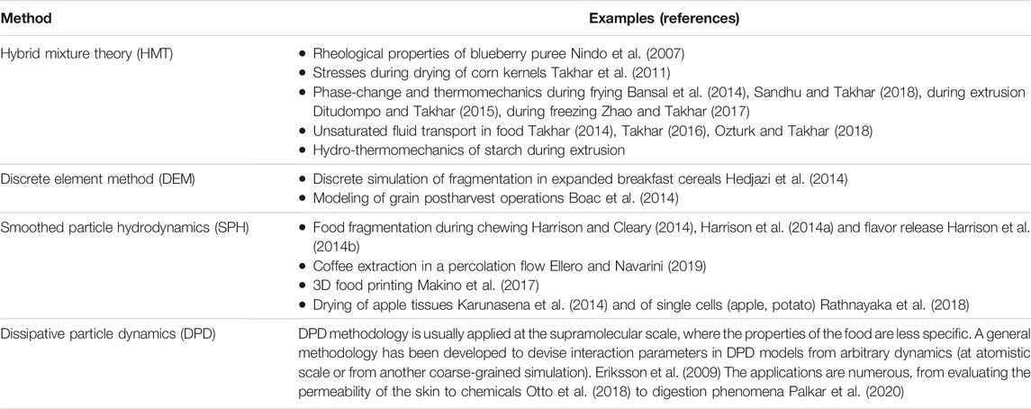
Two families of approximations and simulations have been proposed to address non-heuristically previous limitations, with examples listed in Table 4. The first is the hybrid mixture theory (HMT). This macroscale theory uses constitutive equations, which are neither homogenized nor averaged over the microscale but directly formulated at the macroscale and subjected to the second law of thermodynamics. The approach has been first developed by Hassanizadeh and Gray in seminal papers (Hassanizadeh and Gray, 1979a; Hassanizadeh and Gray, 1979b; Hassanizadeh and Gray, 1980). All conservation equations are averaged using the Whitaker procedure to obtain macroscale field equations, but each variable remains defined precisely in terms of its microscale counterpart. The structure of the theory of mixtures of Bowen (Bowen, 1980; Bowen, 1984) has been implemented to consider the impenetrable/immiscible properties of porous media. Constitutive relations are required to close the formulation, but the approach can be seen as a natural extension of the classical theories of gas mixtures. The formulation is well adapted to describe immiscible and incompressible flows in deformable and rigid solids. For example, capillary pressure can be derived from the free energy of the mixture as a function of temperature, the strain of the solid, and fluid volume fractions. However, HMT proposes closure only for the macroscopic scale and not across the scales. One practical consequence is the lack of conservation of interfacial areas in fractal structures. Hierarchical averaging procedures have been proposed to estimate wetting properties from the microscopic geometry of pores (Gray and Miller, 2005; Miller and Gray, 2005; Gray and Miller, 2006; Miller and Gray, 2008; Gray and Miller, 2009). Though these theories are complex, they highlight the risk of consistency loss in too coarsened models. Keeping thermodynamic constraints across the scales is essential.

TABLE 4

TABLE 4. Examples of direct description of the behavior of multiphasic food properties.

The second family relies on discrete methods to represent inertial flows and complex interactions between solids and fluids. They offer a competitive alternative to the complex description with continuous methods of free surfaces and situations where surface tension dominates (e.g., foaming, coalescence). Discrete mechanics is based on connected objects, points, segments, surfaces, volumes (beads). The positioning of these objects in space is unnecessary, the referential is only local, and the objects are located in relation to each other (Lagrangian description). The corresponding methodologies are essentially meshless, and no spatial discretization is required. Because the variations are numerous, only two methods are briefly presented: discrete element method (DEM) and smoothed particle hydrodynamics (SPH). Both methods rely on collision operators. DEM is the oldest methodology (Cundall and Strack, 1979) and describes dry cohesionless granular flows while accounting for the exact shape of particles. Conversely, SPH is a particle-based continuum method well suited for flows and deformation problems. Continuous media are represented by overlapping particles representing a volume of fluid or solid. The methodology has been initially developed for astrophysical problems (Gingold and Monaghan, 1977; Cleary and Monaghan, 1990). The methodology outperforms any continuous methods to describe free surface flows.

Inherently in the original formulation, the concept of a “blurred” particle suffers several challenges at boundaries and in computational efficiency. It is, therefore, common to represent also solid interfaces with fixed particles. As DEM and SPH simulation methodologies do not rely on statistical ensembles, their original flavors are unsuitable for entropy-driven phenomena. Fluctuations are recovered in Dissipative Particle Dynamics (DPD), which targets all soft-matter and flow phenomena occurring at nanoscale, typically 10 nm–10 μm and 1 ns–1 ms (Español and Warren, 2017). The DPD model, introduced initially by Hoogerbrugge and Koelman (Hoogerbrugge and Koelman, 1992) and subsequently equipped by Español and Warren with a proper statistical mechanics model (Español and Warren, 1995), gained rapid popularity due to its algorithmic simplicity and versatility. Quoting Español and Warren, “just by varying at will the conservative forces between the dissipative particles, one can readily model complex fluids like polymers, colloids, amphiphiles and surfactants, membranes, vesicles, and phase separating fluids. Due to its simple formulation in terms of symmetry principles (Galilean, translational, and rotational invariances), it is a very useful tool to explore generic or universal features (scaling laws, for example) of systems that do not depend on molecular specificity but only on these general principles”. Hence, the interactions in DPD schemes conserve both linear and angular momentum locally. Finally and to be exhaustive, several SDPD “smooth DPD” strategies (Uma et al., 2011; Shang et al., 2012; Donev et al., 2014; Donev and Vanden-Eijnden, 2014) have been explored to get an overlap with SPH methodology.

3 The Problem of Time Homogenization

Quoting Gorban (Gorban et al., 2006), the first coarse-graining algorithm was proposed one century ago by Paul and Tanya Ehrenfest in their paper for the scientific Encyclopedia (Ehrenfest et al., 2014). The operation proposed by the authors transforms the continuous probability density in phase space into a piece-wise function averaged over periodic cells. At the time, averaging over periodic cells was revolutionary as it enabled the system’s entropy to increase even after a long time and overcame the previous limitations offered by the Liouville equation for closed systems. Nowadays, coarse graining over grids is everywhere in statistical physics both at equilibrium and non-equilibrium. Complex transport phenomena (flows, diffusion) can be studied with various dissipation coefficients (viscosity, diffusivities) and decoupled with proper filtering and subgrid modeling.

Strategies that span the time scales in condensed phases follow a different tack than those designed to span spatial scales. Generally, there is a wide gap of about ten orders or more of magnitude in time between processes like atomic vibrations, which ultimately limit simulations at the atomistic scale, and complex diffusion processes that control many dynamic properties such as shelf-life, safety, release digestion, oil uptake, etc. Any robust multiscale modeling strategy should be equipped with both spatial and time homogenization. The key ingredients for time acceleration and ergodicity are:

• to get a proper probabilistic description of first passage times,

• to define the parent stochastic transport mechanism (diffusion, vibrations),

• to set the adequate threshold (energy, filling time, working time),

• to make the time scale emerge from the considered statistical ensemble or the method of sampling,

• to get a proper methodology to sample times continuously.

This section introduces the concepts of transition state theory as a common framework and illustrates several strategies to identify first passage or first hitting times.

3.1 Transition State Theory

Previous methods can zoom spatially continuously from the macroscopic scale down to atoms. Time scale is, however, not treated similarly by modelers as its definition may be twofold. It can date the events since the beginning of the simulation time or our clock time. Still, it can also represent only a reciprocal frequency without specifying the origin of simulation time. This last definition prevails in simulations involving thermodynamic/statistical ensembles, where time emerges directly from free energy variation between two macroscopic states. The dichotomy of time interpretation above a gap ranging from microseconds to milliseconds is shown in Figure 1A. It can be interpreted easily as follows. Macroscopic times define the order of events, while microscopic times are random, and only the durations between events are statistically defined. This memoryless process is called Poissonian and can be sampled causally from a single series of events (e.g., the trajectory from a single particle) or a collection of events (e.g., collection of particles). The difficulty arises from sampling the frequency of rare events (e.g., trapping-release), whose effects control the overall rate or kinetics.

In cohesive systems such as entangled polymers (e.g., packaging walls), structured food systems (e.g., emulsions) or in the presence of chemical reactions (chemisorption, cage effects, etc.), several time scales coexist due to the broad correlations between consecutive phenomena. After coarse-graining, such phenomena can be understood as a macroscopic trap-escape sequence (i.e., collection of macroscopic states), whose frequencies are very low compared to events controlled by the local thermal vibration of atoms or molecules, whose corresponding states are called micro-states. The separation between macro- and microstates on the surface of free energy of the studied system (e.g., mixture) is equivalent to the separation of two different time scales.

Transition-state theory (TST) approximates the rates of a transition between two neighboring macrosites/macrostates, denoted 1 and 2, separated by an asymmetric energy barrier $\mathrm{\Delta }{E}^{1\to \mathrm{‡}}$ and $\mathrm{\Delta }{E}^{2\to \mathrm{‡}}$ as:

$\begin{array}{l}{k}_{\begin{array}{l}\underset{1\to \mathrm{2}}{transition}\end{array}}=\frac{k_{B}T}{h}\frac{Q^{\mathrm{‡}}}{Q_1}\exp \left(-\frac{\mathrm{\Delta }{E}^{\mathrm{1}\to \mathrm{‡}}}{k_{B}T}\right)\\ k_{\begin{array}{l}\underset{2\to \mathrm{1}}{transition}\end{array}}=\frac{k_{B}T}{h}\frac{Q^{\mathrm{‡}}}{Q_2}\exp \left(-\frac{\mathrm{\Delta }{E}^{\mathrm{2}\to \mathrm{‡}}}{k_{B}T}\right),\end{array}(16)$

where $Q^{\mathrm{‡}}$ and ${\left\{Q\right\}}_{i=\mathrm{1,2}}$ are the partition functions of the transition state and the considered macrosite $i$, respectively. $k_B$ and $h$ are the Boltzmann and the Planck constants, respectively; $T$ is the absolute temperature. As partition functions (canonical) are interpreted as the sum of the probabilities in the form of $\exp \left(-\frac{{\mathrm{ϵ}}_j}{k_{B}T}\right)$ with ${\mathrm{ϵ}}_j$ the energy associated to the state $j$, they are likely to be also a function of $T$. TST has been initially devised to calculate reaction rates along a reaction coordinate (Eyring, 1935), and it has been subsequently generalized to the diffusion in glassy polymers (Gray-Weale et al., 1997).

The concept of transition state between macrosites 1 and 2 is essential, and it assumes that the transition paths $1\to 2$ and $2\to 1$ follow the same route and cross a saddle point with negative curvature, denoted $\mathrm{‡}$, where the origin of the motion is indiscernible. The concept of saddle point in classical mechanics assumes that there is a separable coordinate along with the transition occurs (the curvature of the saddle point is positive everywhere except along one coordinate), or more precisely where the flux of probability is maximum in both directions. It corresponds to a favorable collective displacement of atoms or a favorable geometry configuration, suggesting a “tunnel” or a “Red Sea mechanism” connecting two states. By denoting ${\left\{p_i\right\}}_{i=\mathrm{1,2}}$ the equilibrium probability of state $i$, the principle of micro-reversibility reads at any time:

$p_1{k}_{\begin{array}{l}\underset{1\to 2}{transition}\end{array}}=p_2{k}_{\begin{array}{l}\underset{2\to \mathrm{1}}{transition}\end{array}}.(17)$

Once the connectivity of the sites and the frequencies of the corresponding transitions established, the equilibrium distribution can be determined by integrating the macroscopic mass balance equations until to reach steady state $\left(\frac{d{p}_i^{eq}}{dt}=0\right)$:

$\frac{d{p}_i}{dt}={\displaystyle \sum _{jconnectingi}{p}_j{k}_{\begin{array}{l}transition\\ j\to i\end{array}}}-{\displaystyle \sum _{iconnectingj}{p}_i{k}_{\begin{array}{l}transition\\ i\to j\end{array}}}={\displaystyle \sum _{jconnectingi}\left(1-\frac{1}{p_i}\right)}{p}_j{k}_{\begin{array}{l}transition\\ j\to i\end{array}}.(18)$

The asymptotic residence time at any microsite is given by the harmonic average of transition rates:

${\tau }_i=\frac{p_i^{eq}}{{\displaystyle \sum _{iconnectingj}{p}_j^{eq}{k}_{\begin{array}{l}transition\\ j\to i\end{array}}}}=\frac{p_i^{eq}}{{\displaystyle \sum _{iconnectingj}{p}_i^{eq}{k}_{\begin{array}{l}transition\\ i\to j\end{array}}}}=\frac{1}{{\displaystyle \sum _{iconnectingj}{k}_{\begin{array}{l}transition\\ i\to j\end{array}}}}.(19)$

At this stage, it is essential to notice that the TST and the methodology treat time as a continuous variable. Space is replaced by a Lagrangian/Hamiltonian representation via a surface of potential or free (preferred) energy. A continuous representation in time and space can be recovered by averaging the residence times over all possible sites:

$\langle \tau \rangle =\frac{{\displaystyle \sum _{\text{all}i}{p}_i^{eq}}}{{\displaystyle \sum _{\text{all}i}{\displaystyle \sum _{iconnectingj}{k}_{\begin{array}{l}\underset{i\to j}{transition}\end{array}}}}}=\frac{1}{{\displaystyle \sum _{\text{all}i}{\displaystyle \sum _{iconnectingj}{k}_{\begin{array}{l}\underset{i\to j}{transition}\end{array}}}}}.(20)$

Equation 20 lost all microscopic fluctuations describes all transitions as a single uniform random event controlled by an exponential distribution:

$pr\left(t=\mathrm{\Delta }t|\langle t\rangle \right)=\frac{1}{\langle t\rangle }\exp \left(-\frac{\mathrm{\Delta }t}{\langle t\rangle }\right).(21)$

A form of Eq. 21 is applied free-volume theories used to model trace, solute, and mutual diffusion in condensed phases. The probability of a translation (transition) is assumed to be proportional to the probability of a critical amount of free volume accumulating in the immediate vicinity of the considered molecule. The exact position of the atoms and the concept of adjacency do not need to be explicated. Similarly, the dual-mode sorption model assumes that the translation may occur in two different micro-environments (microsites). It might be tempting to consider that Eq. 16 describes a temperature activation of the Arrhenian type. This is not the case because partition functions also contain an enthalpy component. The prefactor describes the effect of thermal agitation as in Stokes-Einstein’s law by a simple temperature effect. The other parameters carry the energy barriers and the effects of thermal expansion. Finally, it deserves to note that multiple transition state theory assumed that the transition rates or, more precisely, that the free energy of interactions is distributed.

3.2 Examples

The following examples illustrate mechanisms involving multiple time scales and the methodology to simulate them by dropping unnecessary details.

3.2.1 Justification of the Separability of Microscopic and Macroscopic Time Scales to Predict Transport Coefficients

Diffusivities of gases and organic molecules in condensed phases (liquids or solids) can be derived from the second-order stationary displacements of the center-of-mass (CM) of one single diffusant (or averaged over the trajectory of several diffusants) by molecular dynamics simulation. The displacements controlling the translation of CM due to thermal noise (collision with atoms of surrounding molecules) between times $\tau$ and $\tau +t$, ${\mathbf{r}}_{\mathbf{CM}}\left(t,\tau \right)$ are defined from the positions vectors (3 × 1 vector) of CM, ${\mathbf{x}}_{CM}$, relatively to the center of mass of the entire system (diffusant + host), ${\mathbf{x}}_O$:

${\mathbf{r}}_{\mathbf{CM}}\left(\tau ,t\right)={\mathbf{x}}_{\mathbf{CM}}\left(\tau +t\right)-{\mathbf{x}}_{\mathbf{CM}}\left(\tau \right)-\left({\mathbf{x}}_{\mathbf{O}}\left(\tau +t\right)-{\mathbf{x}}_{\mathbf{O}}\left(\tau \right)\right).(22)$

When the displacements of CM are truly independent, the quadratic displacement increases linearly with the lag operator $t$ with ${\langle {\mathbf{r}}_{CM}\left(\tau ,t\right)\rangle }_{allt}=0$:

$\frac{d}{dt}{\langle {\mathbf{r}}_{\mathbf{CM}}\left(\tau ,t\right){\mathbf{r}}_{\mathbf{CM}}{\left(\tau ,t\right)}^T\rangle }_{\text{all}\tau }=2\mathbf{D}\left(t\right),(23)$

where $X^T$ is the transpose of $X$. The diffusion matrix $\mathit{D}\left(t\right)$ is positive-defined, whose eigenvectors code for the main direction of translation on time scale $t$. It accepts a unique Cholesky decomposition:

$\mathbf{D}\left(t\right)=\mathbf{B}\left(t\right)\mathbf{\Lambda }{\left(t\right)}^{1/2}{\left(\mathbf{B}\left(t\right)\mathbf{\Lambda }{\left(t\right)}^{1/2}\right)}^T,(24)$

where $\mathbf{\Lambda }\left(t\right)$ is a diagonal matrix containing the eigenvalues and where the columns of $\mathbf{B}\left(t\right)$ are the associated eigenvectors. Displacements fluctuate on the time scale $t$ at a rate $\frac{d{\mathit{r}}_{CM}\left(\tau ,t\right)}{dt}$ equal to $\mathbf{B}\left(t\right)\mathbf{\Lambda }{\left(t\right)}^{\frac{1}{2}}\mathbf{X}$, where $\mathbf{X}$ is a random vector, each of whose components follows a reduced centered normal distribution.

Solutes larger than voids exhibit a preferential direction as shown for methoxybenzene (anisole) in Figure 3, so that the random trajectory looks like an extruded tube on large time scales (Figure 3A). The solute seems to jump from one sorption site to the next, separated by distances ranging from 3 to 6 nm (Figure 3B). During the different jump events, the solute progressively loses memory of its previous orientation (Figure 3D). The macroscopic diffusion coefficient eventually emerges as the trace limit of $\mathbf{D}\left(t\right)$ when $t\to \infty$ (note that $t=\frac{1}{f}$ is the lag operator and not the clock time). By choosing the columns of $\mathbf{B}\left(t\right)$ as reference frame, one gets the following expression of the rate of increase of the mean-square displacement of CM:

$\frac{d}{dt}{\text{msd}}_{\text{CM}}\left(t\right)=\mathrm{tr}\left(\frac{d}{dt}{\langle {\mathbf{r}}_{\mathbf{CM}}\left(\tau ,t\right){\mathbf{r}}_{\mathbf{CM}}{\left(\tau ,t\right)}^T\rangle }_{\text{all}\tau }\right)=2\mathrm{tr}\left(\mathbf{D}\left(t\right)\right)=2\mathrm{tr}\left(\mathbf{\Lambda }\left(t\right)\right)=6D\left(t\right),(25)$

which leads to the practical formula of the macroscopic diffusion $D\left(f=0\right)$:

$D\left(f=0\right)=\frac{1}{6}\underset{t\to \infty }{\lim }\frac{d}{dt}\mathrm{ms}{\mathrm{d}}_{\text{CM}}\left(t\right)\stackrel{\text{large}t}{\approx }\frac{\mathrm{ms}{\mathrm{d}}_{\text{CM}}\left(t\right)}{6t}.(26)$

FIGURE 3

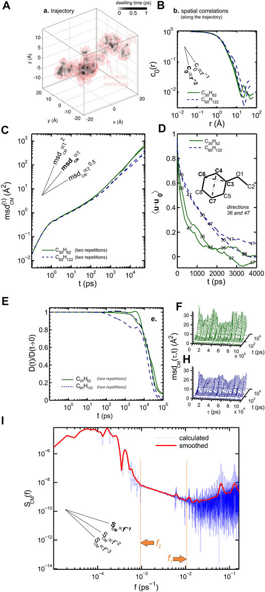
FIGURE 3. Isobaric molecular dynamics simulation of anisole in 20 high-density polyethylene chains at 298 K: (A) residence time mapping; (B) spatial correlation function of residence times; (C) mean-square displacement of the center-of-mass ${\text{msd}}_{\text{CM}}\left(\tau ,t\right)$; (D) correlations of two characteristic vectors of the aromatic ring; (E) evolution of the apparent diffusivity with time scale; (F,H) fluctuations of $ms{d}_{CM}$ with simulated time τ and time scale t; (I) typical fluctuation spectrum $S_{CM}\left(f\right)$ of $\frac{\partial {\text{msd}}_{\text{CM}}}{\partial t}$.

The exponent $\frac{d\text{ ln}\left(ms{d}_{CM}\left(t\right)\right)}{dln\left(t\right)}$ plays a central role in identifying the rate of convergence to the hydrodynamic regime, where all displacements are truly uncorrelated (exponent close to unity). Exponents lower than 1 reveal strongly correlated random walks and apparent diffusivities decreasing with simulation time. Such decreases are shown in Figures 3E–I and occur on a broad range of time scales. The hops responsible for the diffusant translation can be visualized with the spectral density of $\text{d}{\mathbf{r}}_{\text{CM}}/\text{d}\tau$, denoted $S_{CM}\left(f\right)$, which can be calculated from the Wiener-Khinchin real theorem applied to the random variable ${\mathbf{r}}_{\text{CM}}\left(\tau ,t\right)={\displaystyle \underset{\tau }{\overset{\tau +t}{\int }}\text{d}{\mathbf{r}}_{\text{CM}}/\text{d}\tau {|}_{\left(\theta \right)}\text{d}\theta }$. The pair of transforms is known as MacDonald’s theorem [a demonstration is presented in chapter 18 of Ref. (Van Vliet, 2008)] and reads:

$\{\begin{array}{l}\frac{\text{d}}{\text{d}t}\left(\mathrm{ms}{\mathrm{d}}_{\text{CM}}\left(t\right)\right)=2{\displaystyle \underset{0}{\overset{\infty }{\int }}{S}_{CM}\left(f\right)\sin \left(2\pi f\tau \right)}\frac{\text{d}f}{f}\\ S_{CM}\left(f\right)\stackrel{t\to \infty }{=}2f{\displaystyle \underset{0}{\overset{\infty }{\int }}\frac{\text{d}}{\text{dt}}\left(\mathrm{ms}{\mathrm{d}}_{\text{CM}}\left(t\right)\right)\sin \left(2\pi f\tau \right)}\text{d}\tau \end{array}.(27)$

Since the diffusion of a solute larger than voids in a rubber polymer is strongly related to the relaxation of polymer segments, which could think that the convergence of $D\left(t\right)$ should obey some linear damping (e.g., Hooke’s law) and consequently that diffusion coefficients could be easily extrapolated, when the associated time constant $t_0$ is known. This reasoning would lead $S_{CM}\left(f\right)$ to decrease in $\frac{1}{f^2}$ and an exponential convergence to the hydrodynamic regime:

$\{\begin{array}{l}\frac{\text{d}}{\text{d}t}\left(\mathrm{ms}{\mathrm{d}}_{\text{CM}}\left(t\right)\right)=\frac{S_{\text{CM}}\left(f=0\right)}{1-\exp \left(-\frac{t}{t_0}\right)}\\ S_{\text{CM}}\left(f\right)=\frac{S_{\text{CM}}\left(f=0\right)}{1+4{\pi }^2{\left(f{t}_0\right)}^2}\end{array}.(28)$

Figure 3I shows conversely that $S_{CM}\left(f\right)$ evolves from a high-frequency white noise (tumbling motions of the diffusant) towards a low-frequency white noise (macroscopic diffusion) by crossing an intermediate regime linear in $\frac{1}{f}$ (pink noise), separated by two frequencies denoted $f_1$ and $f_2$. This noise corresponds to a random damping process with $t_0$ distributed between $t_2=1/f_2$ and $t_1=1/f_1$, such reasoning leads to:

$\begin{array}{l}\frac{{\displaystyle \underset{t_1}{\overset{t_2}{\int }}{S}_{\text{CM}}\left(f\right)dt}}{t_2-t_1}=\stackrel{t_2>t_1}{=}\frac{S_{\text{CM}}\left(0\right)}{2\pi f\left(t_2-t_1\right)}\left(\arctan 2\pi f{t}_2-\arctan 2\pi f{t}_1\right)\\ =\{\begin{array}{l}\frac{S_{\text{CM}}\left(0\right)}{f^2}\frac{1}{t_1{t}_2}\text{for}f\gg 1/t_2\\ \frac{S_{\text{CM}}\left(0\right)}{4f\left(t_2-t_1\right)}\text{for}1/t_2\ll f\ll 1/t_1\\ S_{\text{CM}}\left(0\right)\text{for}f\ll 1/t_1\end{array}\end{array}(29)$

These results have been used to build a solid theory of diffusion in polymers coupling the free-volume theory and the mode-coupled theory (see Section 4.4). They justify the universal cage-escape mechanism to describe random walks in condensed phases.

3.2.2 Diffusivities on a Surface of Potential: The Relationship Between Diffusion and Sorption at the Molecular Scale

The frequency $f_1\le 1/t_0\le f_2$ and, more particularly, its lower bound control the value of the diffusion coefficient. Ref. (Vitrac and Hayert, 2007) studied the effect of the distribution of sorption energies $G_i$ on $D$ systematically. The frequencies $f_1$ and $f_2$ are connected with the jumping rates via TST, $f=\frac{k_{B}T}{h}\exp \left(-\frac{G_{i\to j}^{\mathrm{‡}}-G_i}{k_{B}T}\right)$, with $G_i$ the local sorption energy at site $i$ and $G_{i\to j}^{\mathrm{‡}}$ the free energy barrier associated to the translation from $i$ to $j$. The main results are illustrated in Figure 4.

FIGURE 4

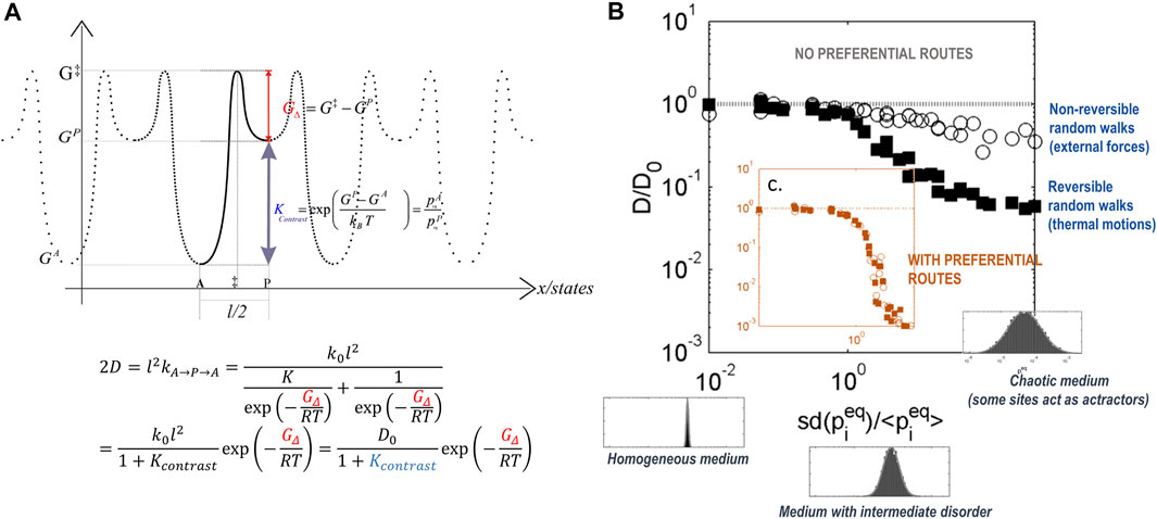
FIGURE 4. Simulation of diffusion using transition state theory in thermoplastic polymers: (A) 1-D diffusion on a 2-state periodic free-energy surface; (B) generalization to 2D random structures where $p_i^{eq}$ is the average probability and $sd\left(p_i^{eq}\right)$ the standard deviation. $D$ and $D_0$ are the diffusivities for heterogeneous and homogeneous media, respectively.

The strong relationship between sorption free energy and diffusion can be easily understood on a periodic surface of free energy, comprising only two states separated by a fixed distance $l$ (Figure 4A). Although it may seem surprising to simulate a random walk on a two-state line, the distance visited is a random variable because the duration of jumps/transitions is also a random variable. The diffusion coefficient depends on two characteristics, the height of the smallest energy barrier $G_{\Delta }$ and the partition coefficient $K_{contrast}$ between the two sites. Increasing $K_{contrast}$ while keeping the same average sorption leads to a dramatic decrease in $D$ values. This effect was verified on random surface energies in higher dimensions. Beyond a critical dispersion value, preferred sites behave as attractors creating negative correlations in the long term. Simulated assumptions are close to what happens when the size of the diffusant is increased (Neyertz and Brown, 2004). On non-random surfaces (i.e., with channels), the reduction of $D$ values is amplified by additional tortuosity effects. Because the results can significantly deviate depending on whether the micro-reversibility hypothesis is verified, it is preferable to restrict the TST approach to the molecular and supramolecular scales. TST-type modeling lends itself very well to the integration of trajectories by Kinetic Monte Carlo (KMC) methods. Classical molecular dynamics simulation and KMC methods can be combined to reproduce the effect of rare events over the long term (Neyertz and Brown, 2010). The methodology allows to obtain statistically independent but without guaranteeing the final $D$ value if limiting events have been insufficiently sampled.

3.2.3 Diffusion in Emulsified Foods

The previous examples justify the concept of time-homogenization to derive macroscopic transport coefficients. Rare events control the entire dynamics and its activation by temperature. One can intuitively think that such phenomena do not exceed a few hundred nanoseconds and are irrelevant at the phase level of the food. This is erroneous because diffusion is a stochastic process in time and in space at all time and length scales. We used to model the diffusion in the hydrodynamic regime in discrete times as a self-similar skewed trajectory, where the direction of the translation and its span are random normal variates. Close to interfaces and, in particular, curved interfaces, the process ceases to be isotropic. By analogy with optics, the constant $K_{contrast}$ and the brusque change of diffusion coefficients at interfaces act as refractive indexes and modify the distribution of molecules on both sides of the interfaces. In dense emulsions with globules close to the percolation threshold, diffusants scatter and reflect towards the medium with the highest residence time. The translation from the medium with the highest diffusion coefficient controls the effective diffusion coefficient. These effects are illustrated in Figure 5 in 1, 2, and 3 dimensions with the following conventions based on the results of Ref. (Vitrac and Hayert, 2020). $K$ is the partition coefficient between the continuous and the dispersed phase. $r_D=\frac{D_c}{D_d}$ is the normalized diffusion coefficient. For large $K$ or low $r_D$ values, the molecules initially contained in the globule create a halo (i.e., close to a diffraction pattern created by an infinitesimal object) around the globule, with a little back diffusion to the reverse direction. At this stage, it is important to notice that $K$ defines only the ratio of diffusant densities across the interface $\partial \Omega$ $\left(x=0\right)$ and not the probability to cross the interface. For the configuration depicted in Figure 5A with a diffusant located initially at $x=x_0$, the ratio of probability to remain the globule after a dimensionless time $Fo=\frac{D_{d}t}{x_0^2}$ is given by:

$\begin{array}{c}\frac{\mathrm{pr}\left(d\to d|\partial \mathrm{\Omega },\text{Fo},x=x_0\right)}{\mathrm{pr}\left(d\to c|\partial \mathrm{\Omega },\text{Fo},x=x_0\right)}=\frac{1}{K}\sqrt{\frac{D_d}{D_c}}\frac{1+\mathit{K}\sqrt{\frac{{\mathit{D}}_{\mathit{d}}}{{\mathit{D}}_{\mathit{c}}}}\mathrm{erf}\left(\frac{1}{2\sqrt{\mathit{Fo}}}\right)}{1-\mathrm{erf}\left(\frac{{\mathit{D}}_{\mathit{d}}}{{\mathit{D}}_{\mathit{c}}}\frac{1}{2\sqrt{\mathit{Fo}}}\right)}\text{exp}\left[-\left(\frac{D_d^2}{D_c^2}-1\right)\frac{1}{Fo}\right]\\ \stackrel{Fo\to \infty }{\to }\frac{1}{K}\sqrt{\frac{D_d}{D_c}}.\end{array}(30)$

FIGURE 5

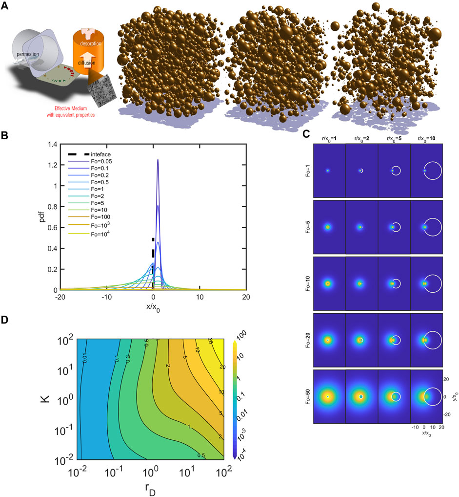
FIGURE 5. Effective diffusivities in emulsions: (A) example of aroma release from 3D emulsions; (B) dimensionless 1D dispersion of a punctual source initially located at $x=x_0>0$ (globule) across the interface $x=0$ for ${\mathit{r}}_{\mathit{D}}$ = $\frac{D_c}{D_d}=4$, $\left(K=2\right)$; (C) corresponding 2D dispersion profiles for different globule sizes; (D) normalized effective diffusivities $D/D_d$ of 3D monodisperse emulsions with a volume fraction of dispersed phase of 0.4. $D$, $D_c$ and $D_d$ are the effective diffusivity, the diffusivity in the continuous and dispersed phase, respectively.

The time limit of Eq. 30 is counter-intuitive and reflects the ability of the diffuser to make countless round trips across the interface but at different speeds. The local thermodynamic equilibrium condition imposes the density ratio (formally $K$) and continuity of the fluxes. Additionally, it is noteworthy that globule interfaces do not represent in this representation a transition state, as the density at the interface is not continuous. However, the global escape rate from each globule could be used as input parameters to simulate diffusion in dispersed media. Compared to Eq. 8, this technique accepts larger fluctuations in surface area, globule size and density, large drops in diffusion coefficients, and finally, partition coefficients very different from unity.

3.2.4 Oil Percolation in French-Fries

Cage-escape mechanisms can be found in various applications, including the percolation of oil in French-fry or potato chips-type products once the product is removed from the bath. Trapped air bubbles in the potato tissue reduce the accessible cross-section to oil and consequently slow down dramatically the capillary flow through crust defects. These effects are illustrated in Figure 6 and are based on simulations and experimental observations reported in (Vauvre et al., 2015) and in (Achir et al., 2010; Vauvre et al., 2014; Patsioura et al., 2015), respectively. We could think that the effective diffusion coefficient of oil should scale as:

$D_o^{\left(z,T\right)}=\langle r\rangle \frac{{\gamma }^{\left(T\right)}\cos \theta }{8{\eta }_o^{\left(T\right)}},(31)$

where here $\gamma$ is the surface tension, $\theta$ the contact angle, ${\eta }_o$ the viscosity of the oil, $\langle r\rangle$ the average radius of cells assuming roughly a cylindrical shape.

FIGURE 6

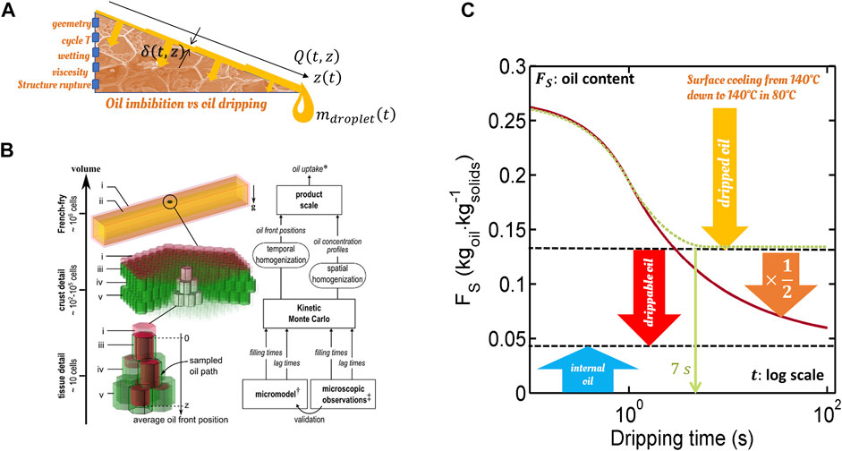
FIGURE 6. Multi-scale modeling of immiscible air-oil flows in fried products: (A) principles of combined modeling of oil absorption and dripping; (B) details of the micro- and macromodels used for oil absorption at cellular scale; (C) possible oil content $F_S$ reduction by increasing oil dripping respectively to oil absorption.

The micro-model showed that the successive filling times of two cavities of radius $r$ and length $\Delta z$ and connected by a defect of radius $r_0$ and length $l_0$ increase considerably with each pass. If the oil-air interface is displaced without creating a bubble (Figure 6A), the recurrence relationship between the filling times $\mathrm{\Delta }{t}_{i,fill}$ is given by:

$\mathrm{\Delta }{t}_{i+1,fill}=\mathrm{\Delta }{t}_{i,fill}-\frac{\ln \left(1-\varsigma \right)}{2\varsigma D_o\left(T\right)}\left(\mathrm{\Delta }\mathrm{z}+l_0{\left(\frac{r}{r_0}\right)}^4\right)\mathrm{\Delta }\mathrm{z},(32)$

with 0 ≤ ς < 1 a factor that controls the gas phase displacement mechanism [see Ref. (Vauvre et al., 2015)].

Due to the hexagonal shape of the cells and the angular details of the defects, the oil flows faster in the corners (Figure 6B) and fills the defects/restrictions without displacing the gas phase. The destabilization of the liquid films in the defects is responsible for the sudden phenomenon of “snap-off” (collapse of two initially disjointed films), which will lead to the creation and trapping of bubbles in the defects. In the presence of an air bubble trapped within the cavity, filling times diverge and Eq. 32 becomes:

$\begin{array}{c}\mathrm{\Delta }{t}_{i+1,fill}^{withbubble}=\mathrm{\Delta }{t}_{i+1,lag}-\frac{\ln \left(1-\varsigma \right)}{2\varsigma D_o}\left(\left(1-\upsilon \right)\mathrm{\Delta }z+l_0{\left(\frac{r}{r_0}\right)}^4\right)\mathrm{\Delta }z\text{ with }\upsilon >0\\ =\mathrm{\Delta }{t}_{i,fill}^{withbubble}-\frac{\ln \left(1-\varsigma \right)}{2\varsigma D_o}\left(\upsilon \mathrm{\Delta }z+l_0{\left(\frac{r}{\xi r_0}\right)}^4\right)\mathrm{\Delta }z-\frac{\ln \left(1-\varsigma \right)}{2\varsigma D_o}\left(\left(1-\upsilon \right)\mathrm{\Delta }z+l_0{\left(\frac{r}{r_0}\right)}^4\right)\mathrm{\Delta }z\\ =\mathrm{\Delta }{t}_{i,fill}^{withbubble}-\frac{\ln \left(1-\varsigma \right)}{2\varsigma D_o}\left(\mathrm{\Delta }z+l_0{\left(\frac{r}{r_0}\right)}^4\left(1+\frac{1}{{\xi }^4}\right)\right)\mathrm{\Delta }z\end{array}(33)$

with $\xi$ the restriction coefficient of the passage related to the presence of the bubble and $\upsilon$ the fraction of the volume of the cell (i.e., formally the cumulative work of the volume forces acting on the bubble) preceding that must flow before the trapped bubble is released. The comparison of Eqs 32, 33 enables to approximate the lag time as $\mathrm{\Delta }{t}_{i+1,lag}\approx \frac{1}{{\xi }^4}\mathrm{\Delta }{t}_{i+1,fill}$ for low values of $\xi$ et $\upsilon$. Experimental filling kinetics of connected cells in parenchyma cells confirm this evolution and the distribution of waiting times as shown in Ref. (Patsioura et al., 2015).

This example and the previous one illustrate the importance of time homogenization and the sampling of rare critical events. Indeed, snap-off and partitioning are elusive and equilibrium properties, respectively. Because its occurrence depends on history, its effects cannot be correctly described by a homogenization procedure, assuming a particular steady-state.

4 Predicting Food and Packaging Properties From Scratch via Molecular Modeling

4.1 Molecular Modeling as an Enabler of Multiscale Modeling

Most of the food industrial and technological processes require including chemical details in models to reach predictive descriptions beyond qualitative ones via dimensionless models. It could be tempting to consider that at the bottom of the hierarchy of the modeling methods across the scales, we have the Hamilton’s equations, their approximate potential energy functions, and the methodology to resolve them numerically via molecular dynamics (MD). Millions to billions of atoms can be simulated nowadays up to hundreds of nanoseconds but not and beyond and at the cost of a time step imposed by the vibration frequency of the hydrogen atom. Brute-force MD is part of the solution but not the solution. Other sampling methodologies, such as thermodynamic integration, particle insertion, non-trivial statistic ensembles, coarse-graining, must be combined to reduce the overall cost of any information added at the atomistic or molecular scale. The blueprint for turning the dream into reality was hypothesized in the eighties by Herschel Rabitz (Rabitz, 1989). The outline of the modeling hierarchy to reproduce bulk observations from atomistic simulations is shown in Figure 7.

FIGURE 7

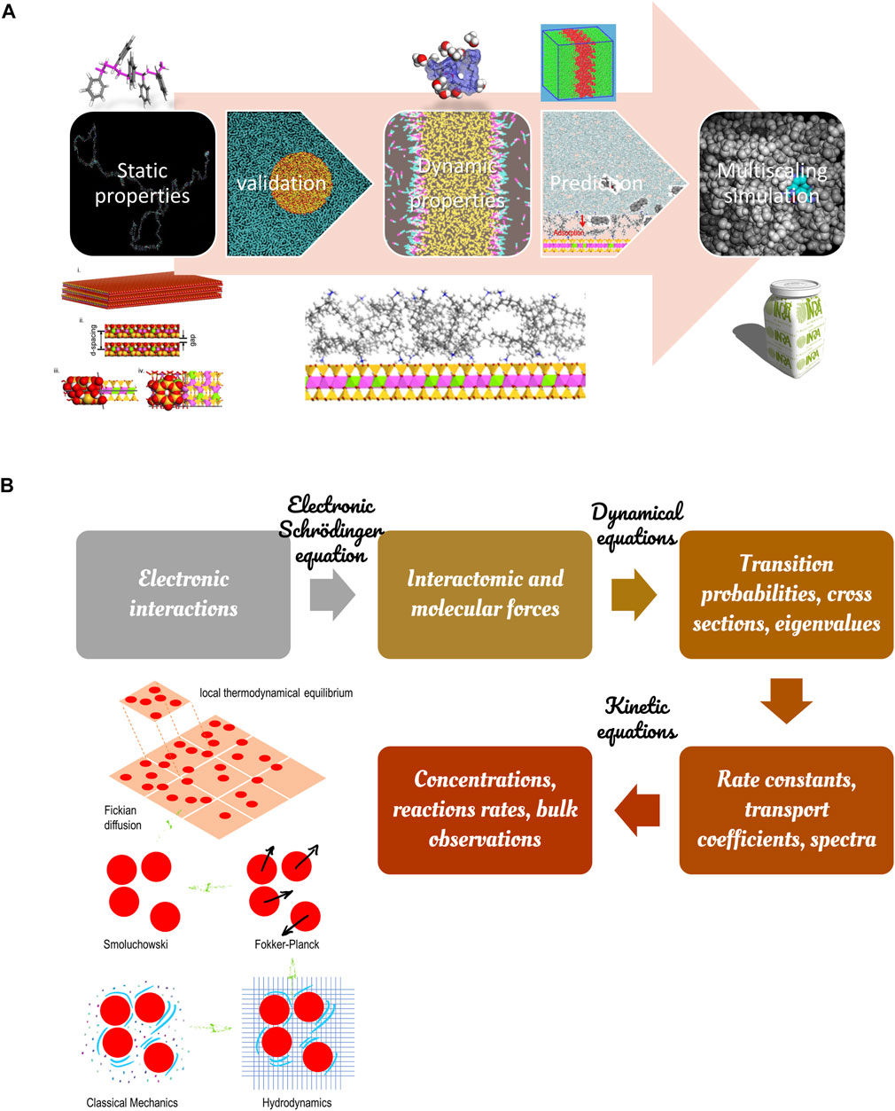
FIGURE 7. Principles to derive bulk properties from atomistic simulations: (A) validation of the static properties of each component before studying the dynamic response of the full system; (B) hierarchy modeling illustrated with the different approximations of Brownian motions (bottom left).

As a general principle, all simulations should validate that the density and pair radial distributions (or structure factor) of pure components are well verified before studying the system’s dynamic response alone or in interactions. This section reviews the experience explored by the authors on molecular modeling and its applicability to food engineering cases. The field is evolving very fast and is the most promising for the future. As already argued by authors (Nguyen et al., 2017a), it starts to be less expensive and faster to launch thermodynamic calculations at the molecular scale than doing the experiments. As discussed in Chapter IV of Ref. (Tadmor and Miller, 2011), molecular dynamics of large systems can be combined or compared with many conventional techniques, such as linear elasticity, nonlinear thermoelasticity, hydrodynamics models of complex fluids, stochastic models with multiple scales, gas-kinetic scheme, quasi-continuum method.

4.2 Principles of Molecular Modeling

Molecular modeling (MM) is an umbrella term covering various techniques, where forcefields bring “life” to simulations, as illustrated in Figure 8. These techniques can be rooted in the seminal works of Martin Karplus, Michael Levitt, and Arieh Warshel, whom the 2013 Nobel Prize has awarded in Chemistry for “the development of multiscale models for complex chemical systems.” A mechanical work leading to displacements of atoms or entities (blobs, group of atoms) can be derived from this potential independently of the path followed by the entire system. Only initial and final steps at the end of each time step count. The considered potentials (between two or more particles) may have several interpretations, quantum or classical, related to hardcore or softcore interactions. This section is not exhaustive but gives an overview of the most relevant techniques for food applications.

FIGURE 8

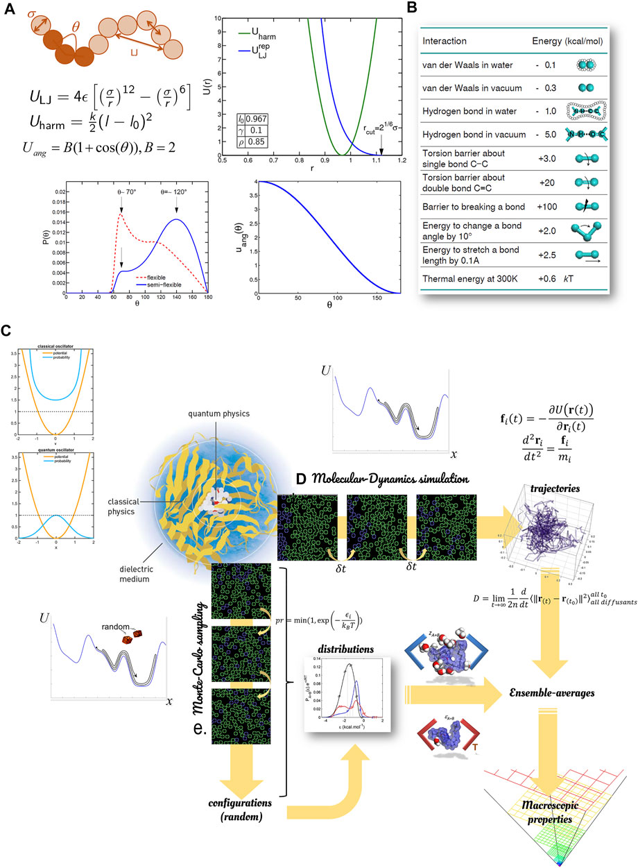
FIGURE 8. Principles of molecular modeling to estimate macroscopic properties in food: (A) example of repulsive forcefields for flexible polymers; (B) indicative interaction energies for non-covalent bonds; (C) macroscopic properties extracted from sampled trajectories; (D) macroscopic properties extracted from sampled configurations.

4.2.1 Forcefields

Molecular modeling uses forcefields to calculate the pair (distance), angular/planar, quadrupole, and octupole interactions between atoms, as sketched in Figure 8A. Most often, forcefields rely on classical Newtonian mechanics. Forcefields representing chemical bonds are either fitted to experimental data (type-I forcefields such as bead-spring model) or fitted to quantum calculations (type-II forcefield with additional corrections to mimic the vibration spectra of molecules). Non-covalent potentials are associated with van-der-Walls and Coulombic interactions defined by partial charges usually applied at the center of atoms. Some software packages, such as LAMMPS (Sandia National Laboratories) and Materials Studio (Dassault Systèmes BIOVIA), offer flexible formulations for soft and solid-state materials and coarse-grain systems. Others, such as Gromacs and Charmm, offers forcefields optimized/specialized for biological molecules, with an emphasis on proteins and lipids. Integrated environments (Avogadro, MedeA LAMMPS from Materials Design, Materials Studio) facilitate the many operations (setup, post-treatments) needed to build and interpret molecular simulations. Some generic visualization tools such as VMD and Ovito offers versatile visualizations for multiscale simulations. For extremely large datasets, the open source ParaView increases the rendering efficiency by focusing on the levels of details important for the observer.

4.2.2 Methods to Explore the Potential Surface

This section introduces briefly the different principles of molecular mechanics. Additional details on forcefields, integration schemes and inversion procedures can be found in the reference textbook of Frenkel and Smit (Frenkel and Smit, 2002). These details are essential to understand the parameterization of open-source (Gromacs, LAMMPS, Charmm, CP2K) or proprietary/commercial software packages (NAMD, Tinker, Materials Studio). At this stage, it is worth noticing that classical oscillators do not behave as quantum ones, whose more probable state coincides with a minimum of potential energy. The likeliest states associated with classical oscillators in dynamics correspond to kinetic energy minima (speed minima) and, therefore, maxima potential energy (see Figure 8C). According to the fluctuation-dissipation theorem, the states corresponding to each maximum are unlikely, but their long-term average in molecular dynamics converges towards the likeliest state at equilibrium. This result will be obtained for microscopically reversible phenomena integrated in time with a time-reversible scheme. However, the convergence to realistic states may be very slow due to explicit numerical schemes, which are stable only for time steps much smaller than the period of the vibration of the lightest atom, typically 1 picosecond in the presence of hydrogens. When trajectories are not required but only configurations or distributions, Monte-Carlo sampling offer atoms better results. It can explore the surface energy in a non-physical manner and overcome any energy barrier separating two feasible states. When the sampling involves a sequence of trial moves (e.g., translation, rotation, volume change), each move must also be picked randomly to enable the reverse course and preserve the detailed balance. The macroscopic quantities are in both cases extracted from ensemble averages.

4.2.3 Coarse-Graining and Boltzmann Inversion

Due to the implicit time integration, acceleration can be gained only by reducing the number of freedoms coupled with longer time steps made possible by merging several atoms (or even molecules) into one heavier particle and therefore subjected to lower frequency vibrations. The iterative coarse-graining methodology is shown in Figure 9. The final goal is to preserve the convergence towards the final property by devising a proper mean force potential ${\varphi }_{CG}\left(R\right)$ from detailed pair energies ${\varphi }_{ij}\left(r_{ij}\right)$. Even if the potential is not defined uniquely, methodologies providing canonical averages will minimize errors on generated configurations, energies, and entropy comparatively to the full detailed ones. Three methodologies have been usually preferred for coarse-graining.

• Direct potential fitting (Cranford et al., 2010): ${\varphi }_{CG}={\displaystyle \sum _{listatoms}{\omega }_{ij}{\varphi }_{ij}}$ where ${\omega }_{ij}$ are summation weights representing all contributions (intramolecular, intermolecular such as hydrophobic and other solvent effects, electrostatic interactions, hydrogen bonding between molecules, and/or entropic effects).

• Inverse Monte-Carlo (McGreevy and Pusztai, 1988) refines iteratively the potential to adjust the pair radial distributions: ${\varphi }_{CG}^{stepk+1}\left(R\right)={\varphi }_{CG}^{stepk}\left(R\right)-a{k}_{B}T\ln \frac{g_{CG}^{stepk}\left(R\right)}{g_{\text{super atoms}}\left(R\right)}$, where $g_{CG}^{stepk}\left(R\right)$ and $g_{\text{super}\text{atoms}}\left(R\right)$ are the radial distribution of the CG model at step $k$ and of the real one, respectively. $a$ is a relaxation constant. In practice, the inversion requires averaging the potential update ${\varphi }_{CG}^{stepk+1}\left(R\right)-{\varphi }_{CG}^{stepk}\left(R\right)$ to all possible configurations of the pair under study.

• Boltzmann inversion (Reith et al., 2003) is a generalization of the previous method to polymers: the Helmholtz free energy $F\left(R\right)=-k_{B}T\ln g_{\text{all}\text{atoms}}\left(R\right)$ is an initial guess for the potential $g_{CG}^{\text{initial}}\left(R\right)$; the methodology is applied separately to intra- and intermolecular potentials (e.g., angular) with an order determined by the intensity of each potential $\left({\varphi }_{CG}^{\text{stretch}}>{\varphi }_{CG}^{\text{bend}}>{\varphi }_{CG}^{\text{non}-\text{bounded}}>{\varphi }_{CG}^{\text{dihedral}}\right)$.

FIGURE 9

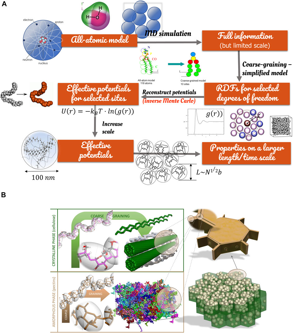
FIGURE 9. Principles of coarse-graining of food constituents: (A) back-mapping from atoms to colloidal systems; (B) examples of coarse-graining applied to crystalline (cellulose) and amorphous constituents (pectins, starch) of potato parenchyma cells.

Though the same methodologies could be applied to adjust forcefields to experimental data, they are presented in a logic of bottom-up modeling and simulation built on molecular mechanics. The knowledge gained at a small scale is used to reconstruct the macroscopic behavior. At small scales, forcefields are inherently repulsive, and the packing of particles is very compact. Excluded volumes vanish at a higher level of coarse-graining, and some overlap must be accepted to preserve the bulk density. At this stage, it is noteworthy that described procedures apply only to conservative forces. Dissipative forces required for DPD simulations must be adjusted to dynamic properties such as viscosity or self-diffusion. Finally, and compared with atomic force fields, coarse-grained forcefields depend on the system’s state (solid, liquid, gas), possibly on temperature and local composition. They are, therefore, not recommended for the calculation of state diagrams without independent validation.

4.2.4 Thermodynamic Equilibrium Between Phases

Studying the effects of temperature and pressure on phase transition is an easy task with the generalization of efficient thermostats and barostats. Enforcing equilibrium between phases in molecular simulation is comparatively much more difficult. Small systems do not behave as large ones. Water did not freeze at the right temperature as it was confined. Water and oil will not create a nice interface within a small cubic simulation box. Droplets are not spherical, and their shape fluctuates with the number and the arrangement of the molecules inside each droplet. Besides, surface tension in droplets smaller than Tolman’s length deviates from its macroscopic value. The finite size of tested systems complicates the construction of large droplets at high dilution. Setting a dimension longer than the two others forces the creation of one flat interface (or two). In this case, the transport of small solutes can be tracked between the two phases at reasonably low concentrations. However, the statistics are too poor to get reliable partition coefficients, and the strategy cannot be generalized to polymers.

Chemical equilibration is the chief difficulty in reaching thermodynamic equilibrium. It requires an exchange of molecules between the two phases. Liquid-vapor and liquid-liquid equilibria can be efficiently studied in the Gibbs ensemble (Panagiotopoulos, 2002) for moderately dense multicomponent fluids. Figure 10 illustrates the principles. The phase coexistence properties of multicomponent systems are studied from a single Monte-Carlo simulation involving two distinct physical regions with different densities and compositions. The regions (boxes) can be dissociated without any common interface. Three types of perturbations are performed on each box: 1) a random displacement of molecules that ensures equilibrium within each region, 2) an equal and opposite change in the volume of the two regions that results in equality of pressures, and 3) random transfers of molecules that equalize the chemical potentials of each component in the two regions.

FIGURE 10

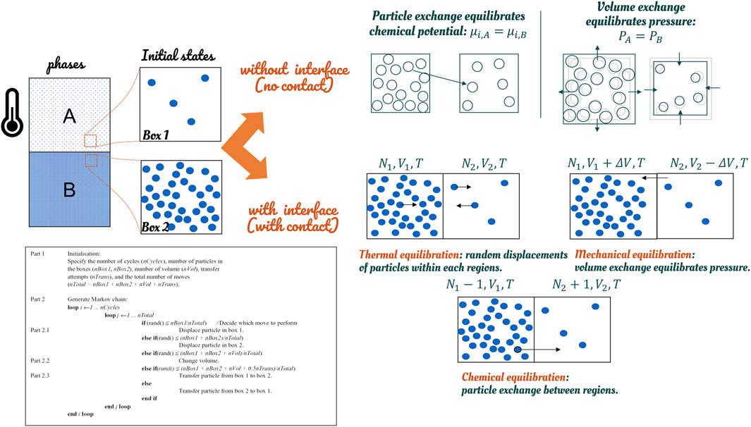
FIGURE 10. Strategies to represent implicitly thermodynamic equilibrium between phases in molecular simulations.

The great advantage of the Gibbs method over the alternative techniques for studying phase coexistence is that, in the Gibbs method, densities and compositions of the coexisting phases are resolved simultaneously. The coexistence line between phases does not require the determination of chemical potentials as a function of temperature and pressure. The list of operations must be picked from a repertoire of trial moves in a random order to preserve the microscopic reversibility. However, the Gibbs ensemble method remains impractical for very cohesive phases such as polymers and very ordered systems (crystals, liquid-crystals). Free-energy calculation methods must be preferred (see Figure 11).

FIGURE 11

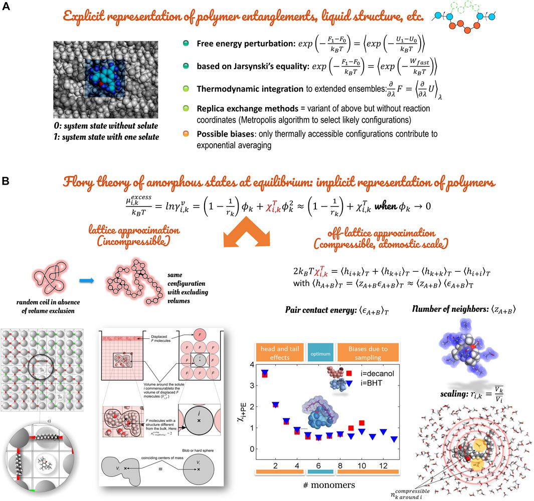
FIGURE 11. Methodologies to calculate activity coefficients and chemical potentials: (A) overview of explicit methods based on Free-energy calculations; (B) implicit method at atomistic scale based on the Flory approximation.

4.3 Calculations of Activity Coefficients Within the Flory Approximation

Activity coefficients and excess chemical potentials are essential properties in food where local composition effects modify strongly how food constituents are transferred inside the food or loss during processing or storage. The same properties control how chemical contaminants are transferred to the food from the packaging or the storage environment. This section reports how the mean-field theory of Flory-Huggins formulated initially on lattices can be turned into a tailored and robust predictive method by using atomistic calculations as inputs. The benefit is twofold. The theory enables first-order predictions without explicitly representing the condensed phase (interacting liquids, entangled polymers). Atomistic calculations with detailed forcefields can replace obsolete group contribution methods and calculations on lattice symmetric imposing symmetric coordination numbers for A surrounding B, and B surrounding A.

4.3.1 Prior Definitions

G. N. Lewis proposed the concept of the thermodynamic potential of substance $i$ in the phase $\alpha$, ${\mu }_{i,\alpha }\left(T,P\right)$, while verifying that ${\frac{\partial {\mu }_{i,\alpha }}{\partial P}|}_T={\overline{V}}_i$ with ${\overline{V}}_i=\frac{RT}{P}$ the molar volume of the gas $i$. After integration at a constant temperature, the change in chemical potential from pressure $P^{ref}$ to $P$ is $RT\ln \frac{P}{P^{ref}}$ for a pure ideal gas. Lewis generalized to phase mixtures (ideal or not) by replacing pressure by a function $f_i$, called fugacity and assessing the capacity of a substance literally to flee: ${\mu }_{i,\alpha }-{\mu }_{i,\alpha }^{ref}=RT\ln \frac{f_{i,\alpha }}{f_{i,\alpha }^{ref}}$. Reference values at the temperature $T$ ${\mu }_{i,\alpha }^{ref}$ and $f_{i,\alpha }^{ref}$ are physically related, but the choice of the reference chemical potential or the reference fugacity is arbitrary. Fugacities of substances absorbed on solids can be determined directly by molecular modeling using the grand-canonical ensemble (μVT). Its utility lies in its resemblance with experimental measurements (e.g., sorption microbalance): the system interchanges particles with a reservoir so that the chemical potential can be by changing the number of particles changes accordingly. As for the Gibbs ensemble, the method is prohibitive for condensed phases. Flory-Huggins’ theory offers a scale-invariant to estimate activity coefficients, ${\gamma }_{i,\alpha }^v$ , relative to volume fractions ${\varphi }_{i,\alpha }$ in any condensed phase, as summarized in Table 5. The presented relationships expressing ${\gamma }_{i,\alpha }^v$ in function of ${\varphi }_{i,\alpha }$ are equivalent to conventional sorption isotherms for binary and ternary mixtures. Indeed, activities and ${\gamma }_{i,\alpha }^v$ are related as:

$\frac{f_{i,\alpha }\left(T\right)}{f_{i,\alpha }^{ref}\left(T\right)}={\gamma }_{i,\alpha }^v\left(T\right){\varphi }_{i,\alpha }.(34)$

TABLE 5

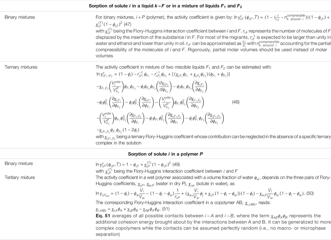
TABLE 5. Relevant binary and ternary Flory isotherms [see details in Ref. (Zhu et al., 2019a)]. The formula applies only to homogeneous phases. For heterogeneous phases (e.g., emulsions), the effective partition coefficient/activity coefficient must be spatially homogenized.

By considering that partial molar volumes are similar in both phases, solute partition coefficients between the phases $\alpha$ and $\beta$ are given by:

$K_{i,\frac{\alpha }{\beta }}^{\left(T\right)}=\frac{{\varphi }_{i,\alpha }/{\overline{V}}_i}{{\varphi }_{i,\beta }/{\overline{V}}_i}=\frac{{\gamma }_{i,\beta }^v\left(T\right)}{{\gamma }_{i,\alpha }^v\left(T\right)}.(35)$

Defining the activity coefficients respectively to volume fractions instead of molar fractions as in the regular solution theory offers several advantages. Volume fractions enable to consider situations where the solute $i$ is larger than surrounding molecules and also the converse situation where $i$ is infinitely smaller than polymer segments. At this stage, it is important to note that the reference state of solute $i$ is an amorphous state. If its reference state is solid at temperature $T$, a fugacity correction equals to the ratio of fugacities between solid and liquid states must be added [see Ref. (Nguyen et al., 2017b)]. Flory-Huggins sorption isotherms are equivalent to Henry ones at infinite dilution and describe well swelling effects (Oswin type isotherms) at high concentrations. Sorption is assumed to be reversible (no hysteresis). Generalization to sorption-desorption cycles with hysteresis when $T_g$ is crossed during sorption can be found in Ref. (Kadam et al., 2014). For liquids, the Kirkwood-Buff (KB) solution theory (Kirkwood and Buff, 1951) at a microscopic scale can provide exact macroscopic predictions even for interacting liquids and vice-versa, as shown by Arieh Ben-Naim (Ben-Naim, 1977). The pro and cons of KB and FH theories are discussed in (Nguyen et al., 2017b). Corrections derived from KB integrals and pair radial distributions are mainly required for compressible mixtures and large solutes, as shown in (Gillet et al., 2010). The term $n_{karoundi}^{compressible}$ captures the positional entropy reduction due to the specific arrangement between a large solute $i$ and the solvent molecules.

4.3.2 Calculation of ${\chi }_{i,k}^T$ at Atomistic Scale

The calculation procedure of excess chemical potentials is summarized in Figure 11, with technical details given in Refs. (Gillet et al., 2009; Gillet et al., 2010; Vitrac and Gillet, 2010; Nguyen et al., 2017a; Nguyen et al., 2017b; Zhu et al., 2019a). The Flory-Huggins isotherm comprises a positional entropy term and an enthalpic term proportional to the extent of ${\left\{{\chi }_{i,k}\right\}}_{k=P,F}$. The first term is determined by the number of molecules $k$, which are displaced by the introduction of $i$ assuming that the mixture is incompressible (first approximation) or compressible (from radial distribution). The second term is essentially enthalpic, but it also contains the non-positional entropic contribution capturing the fluctuations of the contacts between molecules. Both properties can be studied by molecular modeling (packaging of molecules, pair interactions energies). The advantage of the approach is the capacity to extrapolate the results to arbitrary binary, ternary and quaternary composition. Aqueous and hydroalcoholic solutions have been specifically discussed in Ref. (Gillet et al., 2010).

Flory-Huggins coefficients ${\left\{{\chi }_{i,k}\right\}}_{k=P,F}$ are defined as the dimensionless mixing energy (enthalpy) in excess relative to pure compounds; it is defined for polymers ($k=P$) and liquids ($k=F$):

${\chi }_{i,k}^{\left(n_k,T\right)}=\frac{{\langle h_{i+k}^{n_k}\rangle }_T+{\langle h_{k+i}^{n_k}\rangle }_T-{\langle h_{k+k}^{n_k}\rangle }_T-{\langle h_{i+i}\rangle }_T}{2RT}\mathrm{for}k=P,F,(36)$

where ${\langle X\rangle }_T$ represents an ensemble-average of $X$, $n_P$ is the length used in the approximation of the polymer and $n_F=1$.

In agreement with the original Flory approximation, enthalpies ${\langle h_{A+B}\rangle }_T$ are estimated by summing energies of contact ${\mathrm{ϵ}}_{AB}$ when B is contacting the seed molecule A. ${\langle h_{B+A}\rangle }_T$ represents the same energy when B is used as a seed molecule. In practice, ${\mathrm{ϵ}}_{AB}$ is calculated by choosing an orientation randomly for the contact molecule and by translating it along a random line until at least one point of contact is established between the van der Waals surfaces of the contact and seed molecules. The process is repeated for all conformers and stereoisomers considered. Finally, $h_{A+B}$ is estimated as the product of contact energies and the number of neighbors $z_{AB}$ (number of B molecules surrounding A):

${\langle h_{A+B}\rangle }_T={\langle n_{cooperative}{z}_{AB}{\epsilon }_{AB}\rangle }_T\approx n_{cooperative}\langle z_{AB}\rangle {\langle {\epsilon }_{AB}\rangle }_T.(37)$

Equation 37 assumes that ${\mathrm{ϵ}}_{AB}$ and $z_{AB}$ are statically independent (zero covariance). For polymers, the property of independence is achieved with a large enough $n_P$ value so that the surface of contact of the polymer is independent of the length of the considered polymer. The main advantage of the whole approach is that there is no need to represent entanglements in the polymer and free-volume. The shape of the backbone of an infinitely long chain with shorter oligomers prevents head and tail atoms from coming in contact with any van der Waals surface. Cooperative hydrogen bonding is captured by using a value of $n_{cooperative}$ greater than one. The latent heat of vaporization of water can be correctly approximated by ${\langle h_{water+water}\rangle }_T$ using a value of $n_{cooperative}$ different to unity. This value depends on the type of forcefield used to simulate water. As an example, the rigid water model governed by the TIP4P forcefield gives an acceptable value with $n_{cooperative}=1$ whereas $n_{cooperative}=4$ is required with the same forcefield but using three-point charges (forcefield TIP3P). The number 4 reinforces in this case that any water molecule is on average involved in 4 hydrogen bonds of similar strength.

Contact energies are calculated irrespective of any temperature consideration. The effect of temperature is recovered by weighting the distribution of contact energies with the Boltzmann factor $B\left(\mathrm{ϵ}\right)$:

${\langle {\epsilon }_{AB}\rangle }_T=\frac{{\displaystyle \underset{-\infty }{\overset{+\infty }{\int }}pr\left(\epsilon \right)B\left(\epsilon \right)\epsilon d\epsilon }}{{\displaystyle \underset{-\infty }{\overset{+\infty }{\int }}pr\left(\epsilon \right)B\left(\epsilon \right)d\epsilon }}\mathrm{with}B\left(\epsilon \right)=\exp \left(-\epsilon /\left(RT\right)\right).(38)$

At the expense of calculating two integrals, Eq. 38 can be used to estimate ${\chi }_{i,k}^{\left(n_k,T\right)}$ at several temperatures. Conformers need to be generated so that they represent their conformations (radial distribution, constraints of torsion) in the corresponding condensed phase. In practice, they are sampled from molecular dynamics simulations of the equivalent condensed phase.

4.3.3 Examples

The whole approach is versatile and can cover a large number of situations, as exemplified in Figure 12. The study detailed in Ref. (Lu et al., 2008) shows that partition coefficients between a random copolymer material and water are determined for a broad range of organic solutes and isomers. Conventional group methods, such as solubility parameters, drop important molecular details such as structural isomerism, stereoisomerism, tacticity, pattern order, and local chain composition. The examples from Ref. (Nguyen et al., 2017b) show how the calculations can be done inexpensively from homopolymers and then subsequently extended to copolymers (Figure 12A) via Eq. 51 or calculated directly on copolymers (Figure 12B). The results are similar For genuinely random copolymers, and Eq. 51 averages all microscopic contacts, including specific hydrogen bonding, satisfactorily. Nevertheless, mixtures of homopolymers must be considered differently by averaging the energy of mixing and not contact energies, as discussed in the supplementary information of Ref. (Nguyen et al., 2017b).

FIGURE 12

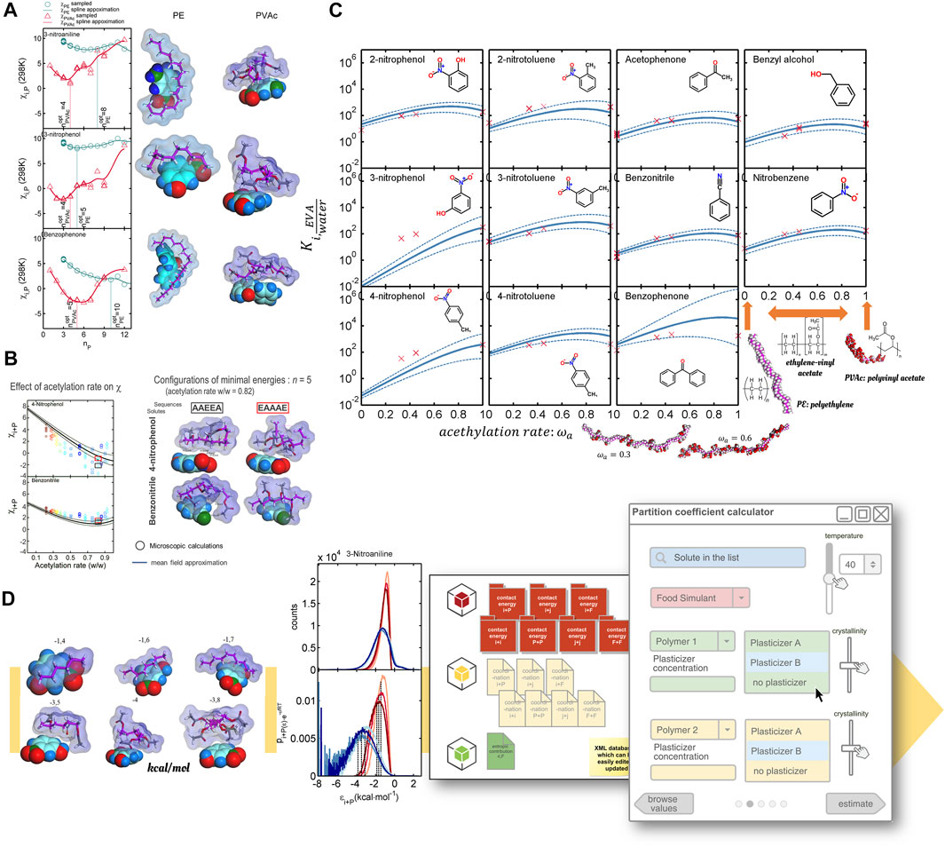
FIGURE 12. Partition coefficients $K_{i,\frac{EVA}{water}}$ calculated at atomistic scale between ethylene-vinyl acetate (EVA) and water: (A) FH coefficient $\left({\chi }_{i,P}\right)$ vs. polymer chain length $\left(n_P\right)$ and pair contact configurations; (B) effect of acetylation rate [continuous curve from Eq. (51); symbols = explicit copolymers]; (C) $K_{i,\frac{EVA}{water}}$ vs. acetylation rate for aromatic solutes; (D) in-house software with a friendly interface and databases precalculated at molecular scale enabling the rapid extrapolation of partition coefficients to arbitrary conditions.

By combining atomistic calculations with Eq. 35, partition coefficients were calculated continuously as a function of the polymer’s acetylation rate. Acetate groups were assumed randomly distributed along the chain. Confidence intervals represent the uncertainty in the convergence of averages with minimum covariances (Figure 12C). Extensive sampling of pair configurations (from several hundred million to several hundred billion) facilitates identifying specific interactions between chemicals. Boltzmann-weighted ensemble averaging (Canonical ensemble) makes it possible to extrapolate sampled results to different temperatures. The only condition is that the conformations of tested conformers remain representative of the state of each component in the mixture. For production, results can be tabulated (sampled pair contact energies, coordination numbers, specific volumes, etc.) and stored for future use. Figure 12D shows the prototype of an in-house software used to calculate partition coefficients between arbitrary plastic materials and food simulants. The calculation procedure is predictive for any organic solute without net charge and prediction errors in the same range as experimental errors. The applicability to food constituents has been tested successfully for starch-water mixtures at rubber state, as met during deep-frying (Nguyen et al., 2017a).

4.4 Free-Volume Theory of Diffusion

4.4.1 Why do We Still Need Theory Instead of Brute Force Calculations?

The concept of free volume is fundamental to liquids and amorphous polymers. Free volumes are defined as the free space between molecules or chain segments; they control important properties of amorphous phases such as their glass transition temperature, their thermal expansion, and their transport properties (White and Lipson, 2016). The law of Stokes-Einstein predicts diffusion coefficients in fluid phases, which are proportional to 1) temperature, 2) the reciprocal viscosity of the liquid, and 3) the reciprocal diameter of the solute. The hydrodynamics theory behind the Stokes-Einstein relationship is, however, not sufficient to illuminate the activation of diffusion by temperature. Indeed, the fluidity (the reciprocal viscosity) or equivalently the friction coefficient is also activated by temperature. Besides, the theory falls short of explaining the extreme mass dependence of diffusivities as observed in amorphous polymers (gels, thermoplastics, thermosets). Although diffusion at constant volume requires a little activation, $k_{B}T$, the cooperation of many degrees of freedom in the host environment is needed to induce the translation of gases or organic solutes larger than surrounding rigid segments. Thermal expansion of van-der-Walls liquids and rubber polymers (ca. 0.1% every 10°C in polyethylene) is the dominant cause of the acceleration of the diffusion in these phases and not directly temperature.

Figure 13 justifies that molecular modeling alone cannot address today all aspects of the mechanism of diffusion for molecules larger than voids in cohesive systems (glasses, entangled polymers). There are two limitations. Firstly, the relaxation modes of entangled polymers or liquids at glassy state cannot be simulated at atomistic scale, as decorrelation times are not accessible to brute force calculations before the next decade. Secondly, large molecules do not translate as a single rigid unit but proceed by small reorientations of internal subunits. A macro-state jump of the center-of-mass succeeds on distances larger than the gyration radius of the diffusant involves, therefore, a large collection of micro-state reorientations. We thought falsely that coarse-graining applied to both the diffusant and the surroundings could alleviate previous time scale limitations. But, because the coarse-graining process removes important atomistic details governing the rate of translation of real diffusants, it created artifacts instead. Log-term molecular dynamics up to 0.06 ms did not succeed in reproducing the strong mass dependence observed at solid-state, as discussed in Ref. (Durand et al., 2010). Heterogeneous dynamics were replaced by smoother ones consistently with Rouse modes observed at molten state when the entire chain of the polymer can translate instead of small segments at solid-state. For example, the displacements of hydrogen atoms along the polyethylene chain control the diffusion rate of helium. In contrast, the shaft motions of connected rigid monomers (-CH₂=CH₂-) govern the translation of methane (CH₄). Larger molecules require activating the relaxation of several polyethylene segments, causing hops to span over a broad range of time scales, as previously discussed in Section 3.2.2.

FIGURE 13

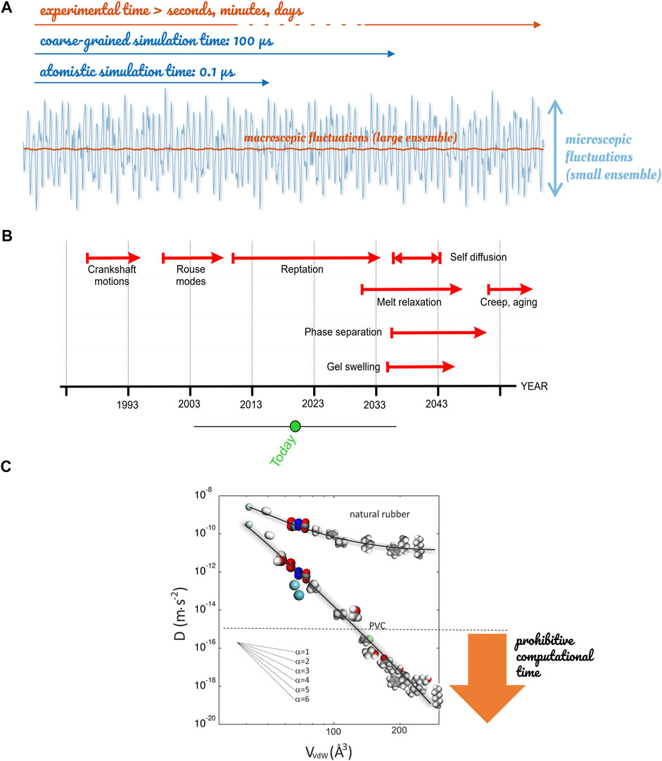
FIGURE 13. Time scale limitations met by atomistic simulations: (A) comparison between macroscopic fluctuations and those accessible today to molecular modeling; (B) projection of capacity of calculations for the next decade in polymers; (C) scaling of diffusion coefficients of gases and organic molecules with their van-der-Waals volume $V_{vdw}$ in rubber (natural rubber) and glassy polymers (polyvinyl chloride: PVC) at 298 K (Berens and Hopfenberg, 1982).

4.4.2 Theory of Vrentas and Duda and its Extensions

Free-volume theory and its extensions, shown in Figure 14, offer an elegant framework to address the problem of many correlations between the translation of the center-of-mass of the solute and the displacements of the surrounding molecules or segments theoretically. Using theory instead of brute force calculations removes restrictions on solute size and the distance to the glass transition temperature $T_g$. The mean-field approximation accepts a rapid parameterization from simple geometry calculations on conformers and solute self-diffusion coefficients determined experimentally or by molecular modeling. By assuming that the translation of a solute is only possible if the free volume fluctuation is larger than a critical volume ${\widehat{V}}^{\ast }$, $D$ is obtained by superimposing all the translation modes for $V\ge {\widehat{V}}^{\ast }$, one gets

$D\left({\widehat{V}}^{\ast }\right)={\displaystyle \underset{{\widehat{V}}^{\ast }}{\overset{+\infty }{\int }}p\left(v\right)D\left(v\right)dv}.(39)$

FIGURE 14

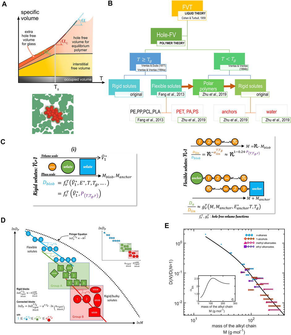
FIGURE 14. Principles of free-volume theory. (A) Interpretation of free volumes in liquids/amorphous polymers at equilibrium (rubber state) and subjected to various degrees of subcooling (glassy state); (B) Connection between the original theory of hole-free volume of diffusion (Cohen and Turnbull, 1959; Vrentas and Duda, 1977b; Vrentas and Vrentas, 1994a; Vrentas and Vrentas, 1994b) and its recent extensions (Fang et al., 2013; Fang and Vitrac, 2017; Zhu et al., 2019b). (C) Principle of decomposition of diffusants in rigid jumping units obeying each the hole-free volume theory. (D) Justification of different scaling relationships of $D$ for solutes with a same molecular mass $M$ but different geometries. (E) Interpretation of the experimental scaling of $D$ for homologous linear solutes with $M$ at 298 K [from Ref. (Zhu et al., 2019b)].

The idea behind Eq. 39 initially postulated by Cohen and Turbull (Cohen and Turnbull, 1959) is that a diffusivity may exist for each type of free volume. We could imagine that all molecules do not translate at the same time to the same fluctuations of free volumes. In the original theory, volumes are expressed in excess of an irreducible volume at a critical temperature $T_{cr}$:

$V_f=V\left(T_{cr}\right)\left(\exp \left({\displaystyle \underset{T_{cr}}{\overset{T}{\int }}\alpha \left(T\right)dT}\right)-1\right),(40)$

where $\alpha \left(T\right)$ is the coefficient of thermal expansion of the fluid. This hypothesis is not realistic in the case of polymers, because the redistribution of interstitial free volumes is associated with relaxation of the polymer chain and thus with very high activation energies (Watanabe, 1999). Vrentas and Duda (Vrentas and Duda, 1977a; Vrentas and Duda, 1977b) removed the objection by arguing that only one hypothetical fraction of free volumes contributed to diffusion; they called it hole-free volumes (hFV). Such theoretical volumes would be redistributed within the polymer without a specific energy barrier. The authors consolidated their theory and arguments during the following 2 decades (Vrentas and Vrentas, 1998). The final theory connects self-diffusion coefficients with mutual and trace diffusion coefficients in liquids and polymers at glassy and rubber states. The canonical formulation for a rigid solute in a rubber polymer at infinite dilution reads [see Ref. (Vrentas and Vrentas, 1998) for details]:

$\begin{array}{c}D=D_0\exp \left(-\frac{E^{\ast }}{RT}\right)\exp \left(-\xi \frac{{\widehat{V}}_2^{\ast }}{{\overline{V}}_{F{H}_2}/{\gamma }_2}\right)\\ =D_0\exp \left(-\frac{E^{\ast }}{RT}\right)\exp \left(-\xi \frac{{\gamma }_2{\widehat{V}}_{22}^{\ast }}{K_{12}\left(T-T_g+K_{22}\right)}\right),\end{array}(41)$

where $\xi {\widehat{V}}_2^{\text{*}}$ is the critical hFV to induce a translation; ${\overline{V}}_{F{H}_2}^{\ast }$ is the critical hFV available for the solute (1) and the polymer (2). $\xi$ is the ratio between the critical volumes of the jumping units of the solute and the polymer.

Because all the parameters can be inferred from quantities independent of the diffusion coefficients or simulated by molecular modeling, it is a predictive and consistent theory from first principles and with Boltzmann statistics. The theory has been later extended (Fang et al., 2013; Fang and Vitrac, 2017; Zhu et al., 2019b) to cover flexible molecules and not only rigid solutes. Earlier mechanisms were kept, a rigid segment can translate or reorient when a void of matching the size of the rigid pattern (blob) opens during redistribution (Fang et al., 2013). The dynamics of the center of mass corresponding to several connected segments is particularly complex as all blobs cannot translate at once. This mechanism was studied by molecular dynamics and mapped onto quantum oscillators to correct the probability of each microstate. The new description predicted successfully that organic solutes (aromatic, aliphatic) in solid polymers would translate with all rigid segments blocked except one. With the help of mode coupled theory, all hFV-related effects were recast in the behavior of linear probes and more specifically in the scaling exponent, ${\alpha }_{lin}$ relating $D$ with the number of connected blobs, as $D\propto M^{-{\alpha }_{lin}}$ (Zhu et al., 2019b):

${\alpha }_{lin}\left(T,T_g\right)\approx 0.24\frac{{\gamma }_2{\widehat{V}}_2^{\ast }}{{\widehat{V}}_{FH2}^{\left(T,T_g\right)}}=0.24\frac{{\gamma }_2{\widehat{V}}_2^{\ast }}{{\text{K}}_{12}}\frac{1}{K_{22}+T-T_g}.(42)$

The revised hFV theory is equipped to capture diffusivities in rubber and glassy polymers of any solute consisting of one single blob or of many blobs of the same size or not, symmetric or not. Figure 15 provides the practical formula and scaling curves valid for 12 polymers (representing the following polymer families: polyolefins, polyesters, polyvinyls, and polyamides). An example of predictions is shown for water in polyethylene terephthalate (PET). The results are remarkable as PET is a polymer, which represents one-third of all food packaging materials; it is the only polymer that can be recycled for food contact so far, and no free-volume theory has been previously published for this polymer. Calculations of the shelf-life of beverages based on diffusion coefficients and sorption isotherms are presented in Ref. (Zhu et al., 2019c).

FIGURE 15

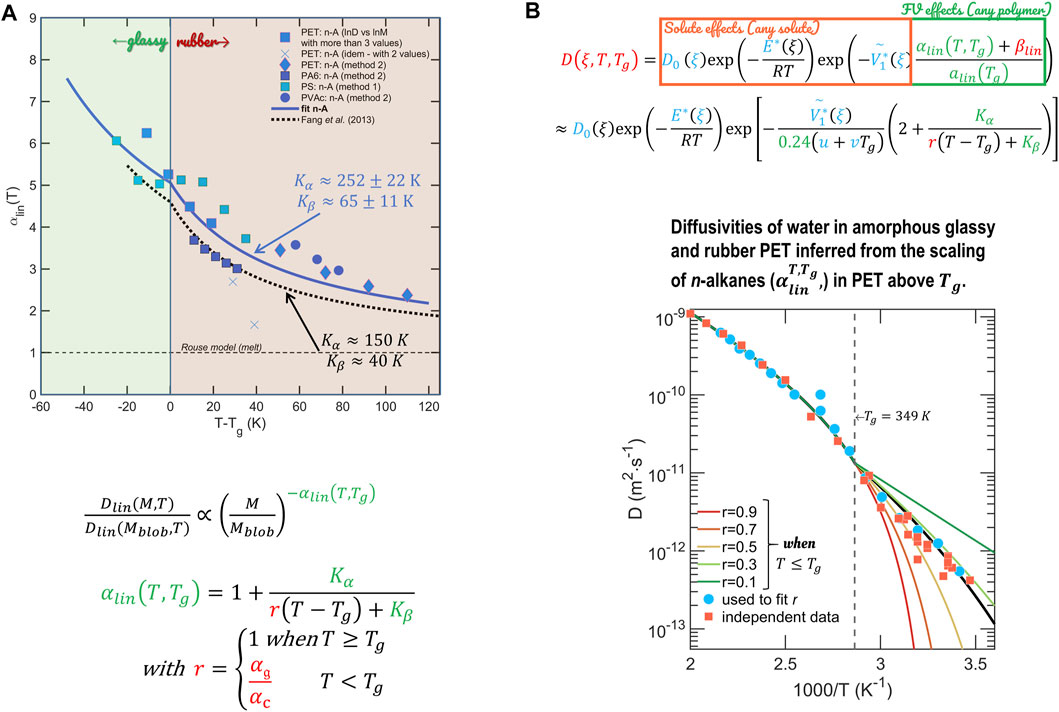
FIGURE 15. (A) Scaling relationship for linear solutes, which are used to probe hole-free volumes in the extended theory of Vrentas and Duda [the two continuous models are from Refs (Fang et al., 2013) and (Zhu et al., 2019b)]; (B) an example of predictions for water in polyethylene terephthalate between 5°C and 190°C. The only degree of freedom is the ratio of thermal expansion between glassy and rubber states, $r$, and characterizing the degree of subcooling of the processed polymer (see Figure 14A). It needs to be fitted or measured independently on the finished product.

5 Guidelines From a Microscopic Perspective

Diffusive or dispersive phenomena have an entropic origin; they are therefore everywhere and characterize the propensity of matter to separate under the effect of thermal agitation. In foods, they are affected by food structure, free volumes, and molecular interactions. The concepts of entropy (thermal, configurational, conformational) are introduced frugally in continuum mechanics via the selection of constitutive laws next to the conservation laws. These constitutive laws are first or second-order approximations of more complex microscopic descriptions, whose complexity is generally reduced to an apparent diffusivity. In the context of food and food packaging, effective diffusivities can range from 10⁻³ to 10⁻¹⁹ m²⋅s⁻¹. This section reviews the strategies for estimating them by adopting a microscopic and mechanistic perspective. The first guidance uses a classification of diffusive phenomena to choose between spatial and temporal homogenization and to suggest a technique. Most concepts are flexible and can be adapted to the phases, domains, species, scales, dimensions, and coupling involved. The second guidance illustrates how apparent radial forces as real as osmotic forces can emerge from microscopic descriptions to describe large classes of entropy-driven problems. This introductive example offers an invitation to discover a highly active research field aiming to understand and control microscopic phenomena.

5.1 Mechanism-Based Strategies to Use and Derive Effective Diffusivities

Analyzing transport properties in foods at all scales at once is either intractable or useless due to the inherent variability of the biological matter. By contrast, replacing microscopic and molecular composite effects with effective diffusivities for relevant geometry domains (skin, crust, core, packaging layer, etc.) allows the use of generic multiphysics simulation software. They are not developed for food products and processes and use continuum mechanics to resolve coupled transfer equations. By repeating the simulations for different property values corresponding to different compositional and structural effects, macroscopic properties of processed foods (e.g., barrier or shelf-life performances) can be related to microscopic or molecular ones and possibly adjusted to reach the desired target. When the properties cannot be tabulated in advance, the effective properties need to be updated regularly. Parallel computing and client-server architecture (usually available in commercial packages) facilitate the development of hierarchical modeling between scales. A whole framework so-called FMECAengine 3D has been developed by us with combine three main loops: one on microscopic properties so-called [E]valuation, a second one [D]ecision devoted to 3D at the macroscopic scale, and a final one [R]esolve relying on multicriteria optimization with microscopic properties as free parameters and product characteristic as goals [see (Zhu et al., 2019c)].

The choice of the appropriate local and global levels, where the equivalent diffusivity is calculated and valid, respectively, remains a challenge. Intuitively, one might think that the smallest level would require the least computational effort (e.g., fastest mixing or decorrelation), but this does not consider the cost of refined details. For most problems, temporal and spatial problems are very intertwined. The chief question is which variable needs absolutely to be considered continuous. As a rule of thumb, it is preferable to consider continuous in-time representations when energy barriers control long waiting time distributions. The following example will show that considering time and space continuous requires introducing proper probability measures. Indeed, what is the probability of two particles moving randomly to meet in diluted regime over a given duration? When a collection of particles are considered, the many interactions problem (collisions are very likely) removes the need for detailed space-time statistics as soon as the density and packaging are well reproduced.

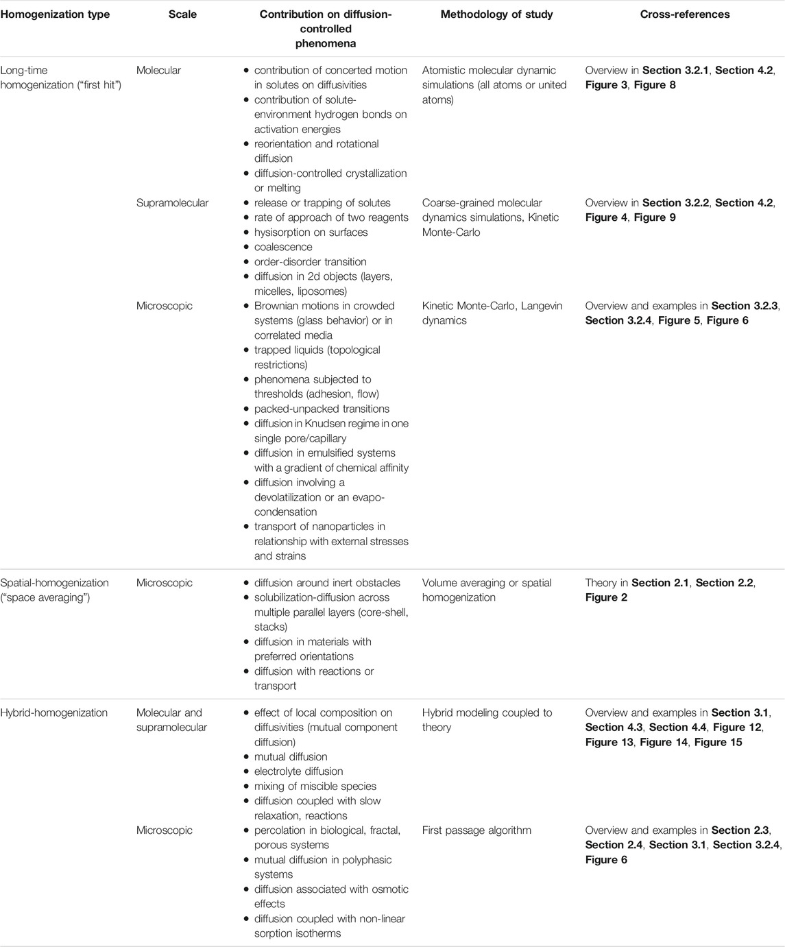
As general guidance, we propose a balance by separating problems above and below the thermodynamic limit (see Figure 1B). Table 6 lists practical strategies to extract effective diffusivities from poor selective mechanisms such as viscous flow, bulk, and Knudsen, surface diffusion to very selective ones such as molecular sieving, capillary condensation, diffusion solubility. Above the thermodynamic limit, diffusion phenomena are self-similar, but scaling remains particularly difficult to predict in the presence of multiple domains, components, or coupling with other driving forces. Below the thermodynamic limit, the many interactions with components, interfaces, and phases may delay the convergence dramatically to the thermodynamic limit and lower diffusivities.

TABLE 6

TABLE 6. Homogenization type for a selection of diffusion-controlled phenomena.

5.2 An Analytical Example of How to Treat Microscopic Mechanisms of Diffusion With Radial Forces

Spatial heterogeneities and viscoelastic relaxation are examples preventing the time and length scales from being separable. They appear in various diffusive phenomena ranging from dissolution to bubble growth. At the microscopic scale, relating the diffusive behavior to the composition gradient as driving forces becomes rapidly impractical. Concentration fields frequently fluctuate due to morphological details (e.g., obstacles, disorder, correlation, network dead-ends), thermodynamic effects (supersaturation, sorption, crystallization … ) and external coupling (osmotic effects, swelling, shear, flow, Marangoni convection). All dispersive phenomena share a common feature: the position and velocity of individual particles cannot be known for sure. The behavior of a single particle can be described in terms of probability density functions in the laboratory-fixed coordinates (via the Fokker-Planck equation) or in a Lagrangian reference frame (via the Langevin equation). However, some concepts are more adapted than others to describe certain phenomena such as order-disorder transitions (mixing, melting, solubilization, elastic behavior). The concept of radial force is one of them and can be deduced from the representation of entropy in statistical mechanics (Neumann, 1980; Roos, 2014).

In the food context, radial forces can be naturally derived and from the differentiation of the chemical potential of one single particle (atom, blob, molecule, fluid volume, colloidal particle), denoted ${\mu }_{1,r}^{\Delta r}$, by assuming that it is located within a spherical shell of radius $r$ and thickness $\Delta r$. For an eventually non-ideal mixture [see the discussion in Ref. (Krishna and Wesselingh, 1997)] and Eq. 39 in Ref. (Zhu et al., 2019a), the magnitude of the radial force reads for each particle:

$f_r=-{\frac{\partial {\mu }_{1,r}^{\Delta r}}{\partial r}|}_T={\mathrm{\Gamma }}_1\frac{k_{B}T}{{\rho }_{1,r}^{\Delta r}}{\frac{\partial {\rho }_{1,r}^{\Delta r}}{\partial r}|}_T={\mathrm{\Gamma }}_1\frac{2k_{B}T}{r},(43)$

where ${\rho }_{1,r}^{\Delta r}=1/\left(4\pi r^2\Delta r\right)$ is the density of one single particle in the shell and ${\mathrm{\Gamma }}_1=1+{\frac{\partial \ln {\gamma }_1^v}{\partial \ln {\varphi }_1}|}_T$ is the thermodynamic factor associated with scaling the activity coefficient ${\gamma }_1^v$ with the volume fraction ${\varphi }_1$.

From Eq. 43, all displacements of species due to chemical potentials (without external forces) can be associated with a radial and centrifugal force with an average magnitude proportional to the reciprocal distance between the source and recipient regions. Conventional descriptions of random walks are recovered by equilibrating $f_r$ with the viscous drag ${\zeta }_1\frac{d\langle r\rangle }{dt}$ associated with the friction coefficient ${\zeta }_1=\frac{k_{B}T}{D_1}$, where $D_1$ is the local diffusivity. Integrating the force balance in spherical coordinates leads to the following differential equation:

$2\mathrm{\Gamma }\langle \frac{1}{r}\rangle =\frac{1}{D_1}\frac{d\langle r\rangle }{dt}.(44)$

Equation 44 is locally valid for any particle following a random walk in a medium governed by $D_1$ and ${\Gamma }_1$. Its integration can be carried out either using Monte-Carlo sampling or with analytical solutions of the probability density function $p_r$, which gives the probability that a particle colliding with its environment reaches a distance between $r$ and $r+dr$ during $t$. For an isotropic, uniform, and infinite medium, the distribution has a Gaussian form:

$p\left(r,t\right)=\frac{4r^2}{\sqrt{\pi }\sigma {\left(t\right)}^3}\exp \left[-{\left(\frac{r}{\sigma \left(t\right)}\right)}^2\right],(45)$

where $\sigma$ is the mode of the distribution (likeliest value of $r$), $\langle r\rangle =\frac{2}{\sqrt{\pi }}\sigma$, $\langle r^2\rangle =\frac{3}{2}{\sigma }^2$, $\langle \frac{1}{r}\rangle =\frac{2}{\sqrt{\pi }}\frac{1}{\sigma }$. Eq. 44 becomes:

$\sigma \left(t\right)d\sigma \left(t\right)=2\mathrm{\Gamma }{D}_{1}dt,(46)$

with the unique solution ${\sigma }^2=4\mathrm{\Gamma }{D}_{1}t$ or equivalently $\langle r^2\rangle =\frac{3}{2}{\sigma }^2=6\mathrm{\Gamma }{D}_{1}t$, which is the same as the Einstein equation for a free random walk for $\mathrm{\Gamma }=1$.

The approach is very general and can be applied to any particle and pair of particles (gel junction, particles representing an interface or an ordered phase) with the addition of proper forces (Coulombic, surface tension, rubber elasticity). In the general case, the distribution is unknown, but it is the most probable distribution maximizing entropy (or the amount of missing information). It can be derived by invoking the central limit theorem or from more straightforward rules. For any finite region divided into cells, the probability of reaching each cell on the long term is proportional to the cell volume divided by the local activity coefficient with a normalization, which depends on the distance to the neighboring regions as shown in Ref. (Vitrac and Hayert, 2020).

6 Conclusion and Perspectives

This article tries to propose some generic recipes for those who want to get into the “mathematical cooking” of food products. The core of the methods consists in presenting how chemical structural information, cell structure and possibly phase organization can be encoded in a coherent mathematical scheme that can be used with classical simulation software at the scale of continuous media. The main tool is the asymptotic analysis. Depending on the importance of the thermodynamic contribution, it must be applied to space or time dimensions. The available computing power necessarily limits the possibilities of prediction and extrapolation but the bricks of a rigorous construction are illustrated. They already offer a significant progress in a context where few properties have been tabulated on raw materials and foods during processing. Indeed modeling and simulation in food is a generally overused term because it means both a descriptive mathematical model and a mechanistic model that can be used to extrapolate, generalize, or even imagine new food products. But the properties are missing at fine scale and the goals can be multifaceted (nutritional, sensorial, cooking behavior, shelf life, health, environmental, etc.). Cooking, drying, freezing and packing food on a computer does not seem very appealing, but the ingredients are there this time. The substances, the macromolecules, the processing conditions can be included in the multi-scale modeling scheme. Not everything can be solved yet, but great steps have been taken in recent years: interactions with models from other disciplines, continuous increase of computing power, many open-source calculation codes, new high-throughput 3D reconstruction tools, more food examples, a better acceptance of model predictions by authorities. The framework is there; now, we must imagine what we can do with the available tools and imagine the new tools we would need for food. We miss quantum methods for foods; they would be beneficial for understanding the complex biochemical reactions that occur during food processing: production of allergens, toxic compounds, depletion of compounds of nutritional interest, digestion, and toxicology of food constituents. This article was written during the Covid-19 pandemic; molecular modeling has been proposed and is in the process of understanding how this new virus works. These new models give us hope that food construction and deconstruction rules can be reviewed very soon.

Data Availability Statement

The original contributions presented in the study are included in the article/Supplementary Material, further inquiries can be directed to the corresponding author.

Author Contributions

All authors contributed on data acquisition and treatment. OV contributed on the redaction of the article. The two others authors contributed to the proofreading.

Conflict of Interest

The authors declare that the research was conducted in the absence of any commercial or financial relationships that could be construed as a potential conflict of interest.

Publisher’s Note

All claims expressed in this article are solely those of the authors and do not necessarily represent those of their affiliated organizations, or those of the publisher, the editors and the reviewers. Any product that may be evaluated in this article, or claim that may be made by its manufacturer, is not guaranteed or endorsed by the publisher.

References

Achir, N., Vitrac, O., and Trystram, G. (2010). Direct Observation of the Surface Structure of French Fries by UV-VIS Confocal Laser Scanning Microscopy. Food Res. Int. 43, 307–314. doi:10.1016/j.foodres.2009.10.004

CrossRef Full Text | Google Scholar

Arrieta-Escobar, J. A., Bernardo, F. P., Orjuela, A., Camargo, M., and Morel, L. (2019). Incorporation of Heuristic Knowledge in the Optimal Design of Formulated Products: Application to a Cosmetic Emulsion. Comput. Chem. Eng. 122, 265–274. doi:10.1016/j.compchemeng.2018.08.032

CrossRef Full Text | Google Scholar

Auriault, J.-L., and Lewandowska, J. (1997). Effective Diffusion Coefficient: From Homogenization to Experiment. Transport in Porous Media 27, 205–223. doi:10.1023/a:1006599410942

CrossRef Full Text | Google Scholar

Baer-Dubowska, W., Bartoszek, A., and Malejka-Giganti, D. (2005). Carcinogenic and Anticarcinogenic Food Components (Chemical and Functional Properties of Food Components Series). Boca Raton, FL: CRC Press.

Google Scholar

Bansal, H. S., Takhar, P. S., and Maneerote, J. (2014). Modeling Multiscale Transport Mechanisms, Phase Changes and Thermomechanics during Frying. Food Res. Int. 62, 709–717. doi:10.1016/j.foodres.2014.04.016

CrossRef Full Text | Google Scholar

Battiato, I., Ferrero V, P. T., O’ Malley, D., Miller, C. T., Takhar, P. S., Valdés-Parada, F. J., et al. (2019). Theory and Applications of Macroscale Models in Porous Media. Transp Porous Med. 130, 5–76. doi:10.1007/s11242-019-01282-2

CrossRef Full Text | Google Scholar

Bazilian, M., Rogner, H., Howells, M., Hermann, S., Arent, D., Gielen, D., et al. (2011). Considering the Energy, Water and Food Nexus: Towards an Integrated Modelling Approach. Energy Policy 39, 7896–7906. doi:10.1016/j.enpol.2011.09.039

CrossRef Full Text | Google Scholar

Ben‐Naim, A. (1977). Inversion of the Kirkwood–Buff Theory of Solutions: Application to the Water–Ethanol System. J. Chem. Phys. 67, 4884–4890.

Google Scholar

Berens, A. R., and Hopfenberg, H. B. (1982). Diffusion of Organic Vapors at Low Concentrations in Glassy PVC, Polystyrene, and PMMA. J. Membr. Sci. 10, 283–303. doi:10.1016/s0376-7388(00)81415-5

CrossRef Full Text | Google Scholar

Bernardo, F. P., and Saraiva, P. M. (2015). A Conceptual Model for Chemical Product Design. Aiche J. 61, 802–815. doi:10.1002/aic.14681

CrossRef Full Text | Google Scholar

Birru, W. A., Warren, D. B., Han, S., Benameur, H., Porter, C. J. H., Pouton, C. W., et al. (2017a). Computational Models of the Gastrointestinal Environment. 2. Phase Behavior and Drug Solubilization Capacity of a Type I Lipid-Based Drug Formulation after Digestion. Mol. Pharmaceutics 14, 580–592. doi:10.1021/acs.molpharmaceut.6b00887

PubMed Abstract | CrossRef Full Text | Google Scholar

Birru, W. A., Warren, D. B., Headey, S. J., Benameur, H., Porter, C. J. H., Pouton, C. W., et al. (2017b). Computational Models of the Gastrointestinal Environment. 1. The Effect of Digestion on the Phase Behavior of Intestinal Fluids. Mol. Pharmaceutics 14, 566–579. doi:10.1021/acs.molpharmaceut.6b00888

PubMed Abstract | CrossRef Full Text | Google Scholar

Boac, J. M., Ambrose, R. P. K., Casada, M. E., Maghirang, R. G., and Maier, D. E. (2014). Applications of Discrete Element Method in Modeling of Grain Postharvest Operations. Food Eng. Rev. 6, 128–149. doi:10.1007/s12393-014-9090-y

CrossRef Full Text | Google Scholar

Bornhorst, G. M., Gouseti, O., Wickham, M. S. J., and Bakalis, S. (2016). Engineering Digestion: Multiscale Processes of Food Digestion. J. Food Sci. 81, R534–R543. doi:10.1111/1750-3841.13216

PubMed Abstract | CrossRef Full Text | Google Scholar

Boulougouris, G. C., Economou, I. G., and Theodorou, D. N. (1999). On the Calculation of the Chemical Potential Using the Particle Deletion Scheme. Mol. Phys. 96, 905–913. doi:10.1080/00268979909483030

CrossRef Full Text | Google Scholar

Boutin, C., and Geindreau, C. (2010). Periodic Homogenization and Consistent Estimates of Transport Parameters through Sphere and Polyhedron Packings in the Whole Porosity Range. Phys. Rev. E 82, 18. doi:10.1103/physreve.82.036313

PubMed Abstract | CrossRef Full Text | Google Scholar

Bowen, R. M. (1980). Incompressible Porous media Models by Use of the Theory of Mixtures. Int. J. Eng. Sci. 18, 1129–1148. doi:10.1016/0020-7225(80)90114-7

CrossRef Full Text | Google Scholar

Bowen, R. M. (1984). Porous Media Model Formulations by the Theory of Mixtures. Netherlands: Springer, 63–119. doi:10.1007/978-94-009-6175-3_2

CrossRef Full Text | Google Scholar

Brewer, P. G., and Peltzer, E. T. (2019). The Molecular Basis for the Heat Capacity and Thermal Expansion of Natural Waters. Geophys. Res. Lett. 46, 13227–13233. doi:10.1029/2019gl085117

CrossRef Full Text | Google Scholar

Burger, J., Papaioannou, V., Gopinath, S., Jackson, G., Galindo, A., and Adjiman, C. S. (2015). A Hierarchical Method to Integrated Solvent and Process Design of Physical CO2 Absorption Using the SAFT ‐γ M Ie Approach. Aiche J. 61, 3249–3269. doi:10.1002/aic.14838

CrossRef Full Text | Google Scholar

Charpentier, J.-C. (2010). Among the Trends for a Modern Chemical Engineering, the Third Paradigm: The Time and Length Multiscale Approach as an Efficient Tool for Process Intensification and Product Design and Engineering. Chem. Eng. Res. Des. 88, 248–254. doi:10.1016/j.cherd.2009.03.008

CrossRef Full Text | Google Scholar

Chen, M., Ko, H.-Y., Remsing, R. C., Calegari Andrade, M. F., Santra, B., Sun, Z., et al. (2017). Ab Initio theory and Modeling of Water. Proc. Natl. Acad. Sci. USA 114, 10846–10851. doi:10.1073/pnas.1712499114

PubMed Abstract | CrossRef Full Text | Google Scholar

Chinesta, F., Torres, R., Ramon, A., Rodrigo, M. C., and Rodrigo, M. (2002). Homogenized thermal Conduction Model for Particulate Foods. Int. J. Therm. Sci. 41, 1141–1150. doi:10.1016/s1290-0729(02)01400-x

CrossRef Full Text | Google Scholar

Cleary, P. W., and Monaghan, J. J. (1990). Toward a Realistic Three-Body Problem. ApJ 349, 150–162. doi:10.1086/168302

CrossRef Full Text | Google Scholar

Clulow, A. J., Parrow, A., Hawley, A., Khan, J., Pham, A. C., Larsson, P., et al. (2017). Characterization of Solubilizing Nanoaggregates Present in Different Versions of Simulated Intestinal Fluid. J. Phys. Chem. B 121, 10869–10881. doi:10.1021/acs.jpcb.7b08622

PubMed Abstract | CrossRef Full Text | Google Scholar

Cohen, M. H., and Turnbull, D. (1959). Molecular Transport in Liquids and Glasses. J. Chem. Phys. 31, 1164–1169. doi:10.1063/1.1730566

CrossRef Full Text | Google Scholar

Conte, E., Gani, R., and Malik, T. I. (2011a). The Virtual Product-Process Design Laboratory to Manage the Complexity in the Verification of Formulated Products. Fluid Phase Equilibria 302, 294–304. doi:10.1016/j.fluid.2010.09.031

CrossRef Full Text | Google Scholar

Conte, E., Gani, R., and Ng, K. M. (2011b). Design of Formulated Products: A Systematic Methodology. Aiche J. 57, 2431–2449. doi:10.1002/aic.12458

CrossRef Full Text | Google Scholar

Cranford, S., and Buehler, M. (2010). “Coarse-Graining Parameterization and Multiscale Simulation of Hierarchical Systems. Part I,” in Multiscale Modeling from Atoms to Devices. Editors P Derosa, and T Cagin (Boca-Raton, FL, USA: CRC Press), 13–34. Chapter 2. doi:10.1201/b10454-3

CrossRef Full Text | Google Scholar

Cummings, P. T., and Evans, D. J. (1992). Nonequilibrium Molecular Dynamics Approaches to Transport Properties and Non-newtonian Fluid Rheology. Ind. Eng. Chem. Res. 31, 1237–1252. doi:10.1021/ie00005a001

CrossRef Full Text | Google Scholar

Cundall, P. A., and Strack, O. D. L. (1979). A Discrete Numerical Model for Granular Assemblies. Géotechnique 29, 47–65. doi:10.1680/geot.1979.29.1.47

CrossRef Full Text | Google Scholar

Datta, A. K. (2007). Porous media Approaches to Studying Simultaneous Heat and Mass Transfer in Food Processes. I: Problem Formulations. J. Food Eng. 80, 80–95. doi:10.1016/j.jfoodeng.2006.05.013

CrossRef Full Text | Google Scholar

Datta, A. K. (2016). Toward Computer-Aided Food Engineering: Mechanistic Frameworks for Evolution of Product, Quality and Safety during Processing. J. Food Eng. 176, 9–27. doi:10.1016/j.jfoodeng.2015.10.010

CrossRef Full Text | Google Scholar

Defraeye, T. (2014). Advanced Computational Modelling for Drying Processes - A Review. Appl. Energ. 131, 323–344. doi:10.1016/j.apenergy.2014.06.027

CrossRef Full Text | Google Scholar

Dickinson, E. (2012). Emulsion Gels: The Structuring of Soft Solids with Protein-Stabilized Oil Droplets. Food Hydrocolloids 28, 224–241. doi:10.1016/j.foodhyd.2011.12.017

CrossRef Full Text | Google Scholar

Dickinson, E. (2008). Interfacial Structure and Stability of Food Emulsions as Affected by Protein-Polysaccharide Interactions. Soft Matter 4, 932. doi:10.1039/b718319d

PubMed Abstract | CrossRef Full Text | Google Scholar

Ditudompo, S., and Takhar, P. S. (2015). Hybrid Mixture Theory Based Modeling of Transport Mechanisms and Expansion-Thermomechanics of Starch during Extrusion. Aiche J. 61, 4517–4532. doi:10.1002/aic.14936

CrossRef Full Text | Google Scholar

Donev, A., Fai, T. G., and Vanden-Eijnden, E. (2014). A Reversible Mesoscopic Model of Diffusion in Liquids: from Giant Fluctuations to Fick's Law. J. Stat. Mech. 2014, P04004. doi:10.1088/1742-5468/2014/04/p04004

CrossRef Full Text | Google Scholar

Donev, A., and Vanden-Eijnden, E. (2014). Dynamic Density Functional Theory with Hydrodynamic Interactions and Fluctuations. J. Chem. Phys. 140, 234115. doi:10.1063/1.4883520

CrossRef Full Text | Google Scholar

Dubbeldam, D., and Snurr, R. Q. (2007). Recent Developments in the Molecular Modeling of Diffusion in Nanoporous Materials. Mol. Simulation 33, 305–325. doi:10.1080/08927020601156418

CrossRef Full Text | Google Scholar

Durand, M., Meyer, H., Benzerara, O., Baschnagel, J., and Vitrac, O. (2010). Molecular Dynamics Simulations of the Chain Dynamics in Monodisperse Oligomer Melts and of the Oligomer Tracer Diffusion in an Entangled Polymer Matrix. J. Chem. Phys. 132, 194902. doi:10.1063/1.3420646

CrossRef Full Text | Google Scholar

Duret, S., Guillier, L., Hoang, H.-M., Flick, D., and Laguerre, O. (2014). Identification of the Significant Factors in Food Safety Using Global Sensitivity Analysis and the Accept-And-Reject Algorithm: Application to the Cold Chain of Ham. Int. J. Food Microbiol. 180, 39–48. doi:10.1016/j.ijfoodmicro.2014.04.009

CrossRef Full Text | Google Scholar

Ehrenfest, P., and Ehrenfest, T. (2014). The Conceptual Foundations of the Statistical Approach in Mechanics, Reprinted from the "Mechanics Enziklopädie der Mathematischen Wissenschaften. P. Ehrenfest, and T. Ehrenfest-Afanasyeva (Leipzig: Dover Publications) Vol. 4, 560p.

Google Scholar

Ellero, M., and Navarini, L. (2019). Mesoscopic Modelling and Simulation of Espresso Coffee Extraction. J. Food Eng. 263, 181–194. doi:10.1016/j.jfoodeng.2019.05.038

CrossRef Full Text | Google Scholar

Engquist, E. W., and Huang, Z. (2003). Heterogeneous Multiscale Method: A General Methodology for Multiscale Modeling. Phys. Rev. B 67, 092101–092104. doi:10.1103/physrevb.67.092101

CrossRef Full Text | Google Scholar

Eriksson, A., Jacobi, M. N., Nyström, J., and Tunstrøm, K. (2009). A Method for Estimating the Interactions in Dissipative Particle Dynamics from Particle Trajectories. J. Phys. Condens. Matter 21, 095401. doi:10.1088/0953-8984/21/9/095401

CrossRef Full Text | Google Scholar

ESA(2017). How many Stars Are There in the Universe. Available from: https://www.esa.int/Science_Exploration/Space_Science/Herschel/How_many_stars_are_there_in_the_Universe#.YYknM_GE_A0.link (Accessed November 08, 2021).

Google Scholar

Español, P., and Warren, P. B. (2017). Perspective: Dissipative Particle Dynamics. J. Chem. Phys. 146, 150901. doi:10.1063/1.4979514

CrossRef Full Text | Google Scholar

Español, P., and Warren, P. (1995). Statistical Mechanics of Dissipative Particle Dynamics. Europhys. Lett. 30, 191–196. doi:10.1209/0295-5075/30/4/001

CrossRef Full Text | Google Scholar

Eyring, H. (1935). The Activated Complex in Chemical Reactions. J. Chem. Phys. 3, 107–115. doi:10.1063/1.1749604

CrossRef Full Text | Google Scholar

Fan, C. F., Olafson, B. D., Blanco, M., and Hsu, S. L. (1992). Application of Molecular Simulation to Derive Phase Diagrams of Binary Mixtures. Macromolecules 25, 3667–3676. doi:10.1021/ma00040a010

CrossRef Full Text | Google Scholar

Fang, X., Domenek, S., Ducruet, V., Réfrégiers, M., and Vitrac, O. (2013). Diffusion of Aromatic Solutes in Aliphatic Polymers above Glass Transition Temperature. Macromolecules 46, 874–888. doi:10.1021/ma3022103

CrossRef Full Text | Google Scholar

Fang, X., and Vitrac, O. (2017). Predicting Diffusion Coefficients of Chemicals in and through Packaging Materials. Crit. Rev. Food Sci. Nutr. 57, 275–312. doi:10.1080/10408398.2013.849654

PubMed Abstract | CrossRef Full Text | Google Scholar

Frenkel, D., and Smit, B. (2002). Understanding Molecular Simulation: From Algorithms to Applications. 2nd Edition. San Diego: Elsevier Science.

Google Scholar

Frenkel, D. (2014). Why Colloidal Systems Can Be Described by Statistical Mechanics: Some Not Very Original Comments on the Gibbs Paradox. Mol. Phys. 112, 2325–2329. doi:10.1080/00268976.2014.904051

CrossRef Full Text | Google Scholar

Gautieri, A., Ionita, M., Silvestri, D., Votta, E., Vesentini, S., Fiore, G. B., et al. (2010). Computer-Aided Molecular Modeling and Experimental Validation of Water Permeability Properties in Biosynthetic Materials. Jnl Comp. Theo Nano 7, 1287–1293. doi:10.1166/jctn.2010.1482

CrossRef Full Text | Google Scholar

Ge, S., Wang, N., Fung, K. Y., Wong, K. W., Chan, C. T., and Ng, K. M. (2018). Product Design: Nanoparticle-Loaded Polyvinyl Butyral Interlayer for Solar Control. AIChE J. 64, 3614–3624. doi:10.1002/aic.16329

CrossRef Full Text | Google Scholar

Gear, C. W., Hyman, J. M., Kevrekidid, P. G., Kevrekidis, I. G., Runborg, O., and Theodoropoulos, C. (2003). Equation-Free, Coarse-Grained Multiscale Computation: Enabling Mocroscopic Simulators to Perform System-Level Analysis. Commun. Math. Sci. 1, 715–762. doi:10.4310/CMS.2003.v1.n4.a5

CrossRef Full Text | Google Scholar

Gerbaud, V., Teles Dos Santos, M., Pandya, N., and Aubry, J. M. (2017). Computer Aided Framework for Designing Bio-Based Commodity Molecules with Enhanced Properties. Chem. Eng. Sci. 159, 177–193. doi:10.1016/j.ces.2016.04.044

CrossRef Full Text | Google Scholar

Gillet, G., Vitrac, O., and Desobry, S. (2010). Prediction of Partition Coefficients of Plastic Additives between Packaging Materials and Food Simulants. Ind. Eng. Chem. Res. 49, 7263–7280. doi:10.1021/ie9010595

CrossRef Full Text | Google Scholar

Gillet, G., Vitrac, O., and Desobry, S. (2009). Prediction of Solute Partition Coefficients between Polyolefins and Alcohols Using a Generalized Flory−Huggins Approach. Ind. Eng. Chem. Res. 48, 5285–5301. doi:10.1021/ie801141h

CrossRef Full Text | Google Scholar

Gingold, R. A., and Monaghan, J. J. (1977). Smoothed Particle Hydrodynamics: Theory and Application to Non-spherical Stars. Monthly Notices R. Astronomical Soc. 181, 375–389. doi:10.1093/mnras/181.3.375

CrossRef Full Text | Google Scholar

Gorban, A. N., Kazantzis, N., Kevrekidis, I. G., Öttinger, H. C., and Theodoropoulos, K. (2006). Model Reduction and Coarse-Graining Approaches for Multiscale Phenomena. Berlin Heidelberg: Springer.

Google Scholar

Gray, W. G., and Miller, C. T. (2005). Thermodynamically Constrained Averaging Theory Approach for Modeling Flow and Transport Phenomena in Porous Medium Systems: 1. Motivation and Overview. Adv. Water Resour. 28, 161–180. doi:10.1016/j.advwatres.2004.09.005

CrossRef Full Text | Google Scholar

Gray, W. G., and Miller, C. T. (2006). Thermodynamically Constrained Averaging Theory Approach for Modeling Flow and Transport Phenomena in Porous Medium Systems: 3. Single-fluid-phase Flow. Adv. Water Resour. 29, 1745–1765. doi:10.1016/j.advwatres.2006.03.010

CrossRef Full Text | Google Scholar

Gray, W. G., and Miller, C. T. (2009). Thermodynamically Constrained Averaging Theory Approach for Modeling Flow and Transport Phenomena in Porous Medium Systems: 5. Single-fluid-phase Transport. Adv. Water Resour. 32, 681–711. doi:10.1016/j.advwatres.2008.10.013

PubMed Abstract | CrossRef Full Text | Google Scholar

Gray-Weale, A. A., Henchman, R. H., Gilbert, R. G., Greenfield, M. L., and Theodorou, D. N. (1997). Transition-State Theory Model for the Diffusion Coefficients of Small Penetrants in Glassy Polymers. Macromolecules 30, 7296–7306. doi:10.1021/ma970349f

CrossRef Full Text | Google Scholar

Greiner, M., Sonnleitner, B., Mailänder, M., and Briesen, H. (2014). Modeling Complex and Multi-Component Food Systems in Molecular Dynamics Simulations on the Example of Chocolate Conching. Food Funct. 5, 235–242. doi:10.1039/c3fo60355e

PubMed Abstract | CrossRef Full Text | Google Scholar

Gulati, T., and Datta, A. K. (2013). Enabling Computer-Aided Food Process Engineering: Property Estimation Equations for Transport Phenomena-Based Models. J. Food Eng. 116, 483–504. doi:10.1016/j.jfoodeng.2012.12.016

CrossRef Full Text | Google Scholar

Haidvogel, D. B., Curchitser, E. N., Danilov, S., and Fox-Kemper, B. (2017). Numerical Modelling in a Multiscale Ocean. J Mar. Res. 75, 683–725. doi:10.1357/002224017823523964

CrossRef Full Text | Google Scholar

Han, J., Gee, R. H., and Boyd, R. H. (1994). Glass Transition Temperatures of Polymers from Molecular Dynamics Simulations. Macromolecules 27, 7781–7784. doi:10.1021/ma00104a036

CrossRef Full Text | Google Scholar

Harrison, S. M., and Cleary, P. W. (2014). Towards Modelling of Fluid Flow and Food Breakage by the Teeth in the Oral Cavity Using Smoothed Particle Hydrodynamics (SPH). Eur. Food Res. Technol. 238, 185–215. doi:10.1007/s00217-013-2077-8

CrossRef Full Text | Google Scholar

Harrison, S. M., Eyres, G., Cleary, P. W., Sinnott, M. D., Delahunty, C., and Lundin, L. (2014a). Computational Modeling of Food Oral Breakdown Using Smoothed Particle Hydrodynamics. J. Texture Stud. 45, 97–109. doi:10.1111/jtxs.12062

CrossRef Full Text | Google Scholar

Harrison, S. M., Cleary, P. W., Eyres, G., D. Sinnott, M., and Lundin, L. (2014b). Challenges in Computational Modelling of Food Breakdown and Flavour Release. Food Funct. 5, 2792–2805. doi:10.1039/c4fo00786g

PubMed Abstract | CrossRef Full Text | Google Scholar

Hassanizadeh, M., and Gray, W. G. (1979a). General Conservation Equations for Multi-phase Systems: 1. Averaging Procedure. Adv. Water Resour. 2, 131–144. doi:10.1016/0309-1708(79)90025-3

CrossRef Full Text | Google Scholar

Hassanizadeh, M., and Gray, W. G. (1979b). General Conservation Equations for Multi-phase Systems: 2. Mass, Momenta, Energy, and Entropy Equations. Adv. Water Resour. 2, 191–203. doi:10.1016/0309-1708(79)90035-6

CrossRef Full Text | Google Scholar

Hassanizadeh, M., and Gray, W. G. (1980). General Conservation Equations for Multi-phase Systems: 3. Constitutive Theory for Porous media Flow. Adv. Water Resour. 3, 25–40. doi:10.1016/0309-1708(80)90016-0

CrossRef Full Text | Google Scholar

Hatch, F. T., and Colvin, M. E. (1997). Quantitative Structure-Activity (QSAR) Relationships of Mutagenic Aromatic and Heterocyclic Amines. Mutat. Research/Fundamental Mol. Mech. Mutagenesis 376, 87–96. doi:10.1016/s0027-5107(97)00029-8

CrossRef Full Text | Google Scholar

Hedjazi, L., Martin, C. L., Guessasma, S., Della Valle, G., and Dendievel, R. (2014). Experimental Investigation and Discrete Simulation of Fragmentation in Expanded Breakfast Cereals. Food Res. Int. 55, 28–36. doi:10.1016/j.foodres.2013.10.025

CrossRef Full Text | Google Scholar

Heintz, J., Belaud, J.-P., and Gerbaud, V. (2014). Chemical enterprise Model and Decision-Making Framework for Sustainable Chemical Product Design. Comput. Industry 65, 505–520. doi:10.1016/j.compind.2014.01.010

CrossRef Full Text | Google Scholar

Ho, Q. T., Verboven, P., Verlinden, B. E., Herremans, E., Wevers, M., Carmeliet, J., et al. (2011). A Three-Dimensional Multiscale Model for Gas Exchange in Fruit. Plant Physiol. 155, 1158–1168. doi:10.1104/pp.110.169391

PubMed Abstract | CrossRef Full Text | Google Scholar

Holmboe, M., Larsson, P., Anwar, J., and Bergström, C. A. S. (2016). Partitioning into Colloidal Structures of Fasted State Intestinal Fluid Studied by Molecular Dynamics Simulations. Langmuir 32, 12732–12740. doi:10.1021/acs.langmuir.6b03008

PubMed Abstract | CrossRef Full Text | Google Scholar

Hoogerbrugge, P. J., and Koelman, J. M. V. A. (1992). Simulating Microscopic Hydrodynamic Phenomena with Dissipative Particle Dynamics. Europhys. Lett. 19, 155–160. doi:10.1209/0295-5075/19/3/001

CrossRef Full Text | Google Scholar

Jang, Y. H., Hwang, S., Chang, S. B., Ku, J., and Chung, D. S. (2009). Acid Dissociation Constants of Melamine Derivatives from Density Functional Theory Calculations. J. Phys. Chem. A. 113, 13036–13040. doi:10.1021/jp9053583

CrossRef Full Text | Google Scholar

Jonuzaj, S., Cui, J., and Adjiman, C. S. (2019). Computer-aided Design of Optimal Environmentally Benign Solvent-Based Adhesive Products. Comput. Chem. Eng. 130, 106518. doi:10.1016/j.compchemeng.2019.106518

CrossRef Full Text | Google Scholar

Jung, J., Nishima, W., Daniels, M., Bascom, G., Kobayashi, C., Adedoyin, A., et al. (2019). Scaling Molecular Dynamics beyond 100,000 Processor Cores for Large‐scale Biophysical Simulations. J. Comput. Chem. 40, 1919–1930. doi:10.1002/jcc.25840

PubMed Abstract | CrossRef Full Text | Google Scholar

Kadam, A., Karbowiak, T., Voilley, A., Bellat, J.-P., Vitrac, O., and Debeaufort, F. (2014). Sorption Ofn-Hexane in Amorphous Polystyrene. J. Polym. Sci. Part. B: Polym. Phys. 52, 1252–1258. doi:10.1002/polb.23557

CrossRef Full Text | Google Scholar

Kalakul, S., Zhang, L., Fang, Z., Choudhury, H. A., Intikhab, S., Elbashir, N., et al. (2018). Computer Aided Chemical Product Design - ProCAPD and Tailor-Made Blended Products. Comput. Chem. Eng. 116, 37–55. doi:10.1016/j.compchemeng.2018.03.029

CrossRef Full Text | Google Scholar

Kanit, T., N’Guyen, F., Forest, S., Jeulin, D., Reed, M., and Singleton, S. (2006). Apparent and Effective Physical Properties of Heterogeneous Materials: Representativity of Samples of Two Materials from Food Industry. Comp. Methods Appl. Mech. Eng. 195, 3960–3982. doi:10.1016/j.cma.2005.07.022

CrossRef Full Text | Google Scholar

Karunasena, H. C. P., Senadeera, W., Brown, R. J., and Gu, Y. T. (2014). A Particle Based Model to Simulate Microscale Morphological Changes of Plant Tissues during Drying. Soft Matter 10, 5249–5268. doi:10.1039/c4sm00526k

PubMed Abstract | CrossRef Full Text | Google Scholar

Keffer, D. J., Edwards, B. J., and Adhangale, P. (2004). Determination of Statistically Reliable Transport Diffusivities from Molecular Dynamics Simulation. J. Non-Newtonian Fluid Mech. 120, 41–53. doi:10.1016/j.jnnfm.2004.01.014

CrossRef Full Text | Google Scholar

Kevrekidis, I. G., and Samaey, G. (2009). Equation-Free Multiscale Computation: Algorithms and Applications. Annu. Rev. Phys. Chem. 60, 321–344. doi:10.1146/annurev.physchem.59.032607.093610

PubMed Abstract | CrossRef Full Text | Google Scholar

Kirkwood, J. G., and Buff, F. P. (1951). The Statistical Mechanical Theory of Solutions. I. J. Chem. Phys. 19, 774–777. doi:10.1063/1.1748352

CrossRef Full Text | Google Scholar

Kontogeorgis, G. M., and Folas, G. K. (2010). Thermodynamics for Process and Product DesignThermodynamic Models for Industrial Applications. Chichester, UK: John Willey & Sons, 1–15.

Google Scholar

Kontogeorgis, G. M., Mattei, M., Ng, K. M., and Gani, R. (2019). An Integrated Approach for the Design of Emulsified Products. Aiche J. 65, 75–86. doi:10.1002/aic.16363

CrossRef Full Text | Google Scholar

Kossack, S., Kraemer, K., Gani, R., and Marquardt, W. (2008). A Systematic Synthesis Framework for Extractive Distillation Processes. Chem. Eng. Res. Des. 86, 781–792. doi:10.1016/j.cherd.2008.01.008

CrossRef Full Text | Google Scholar

Krishna, R., and Wesselingh, J. A. (1997). The Maxwell-Stefan Approach to Mass Transfer. Chem. Eng. Sci. 52, 861–911. doi:10.1016/s0009-2509(96)00458-7

CrossRef Full Text | Google Scholar

Laguerre, O., Hoang, H. M., and Flick, D. (2013). Experimental Investigation and Modelling in the Food Cold Chain: Thermal and Quality Evolution. Trends Food Sci. Techn. 29, 87–97. doi:10.1016/j.tifs.2012.08.001

CrossRef Full Text | Google Scholar

Lee, C. K. H., Choy, K. L., and Chan, Y. N. (2014). A Knowledge-Based Ingredient Formulation System for Chemical Product Development in the Personal Care Industry. Comput. Chem. Eng. 65, 40–53. doi:10.1016/j.compchemeng.2014.03.004

CrossRef Full Text | Google Scholar

Lee, C. T., and Amaro, R. E. (2018). Exascale Computing: A New Dawn for Computational Biology. Comput. Sci. Eng. 20, 18–25. doi:10.1109/mcse.2018.05329812

PubMed Abstract | CrossRef Full Text | Google Scholar

Lee, W. B., Mezzenga, R., and Fredrickson, G. H. (2007). Anomalous Phase Sequences in Lyotropic Liquid Crystals. Phys. Rev. Lett. 99, 187801. doi:10.1103/PhysRevLett.99.187801

PubMed Abstract | CrossRef Full Text | Google Scholar

Lu, P. J., Zaccarelli, E., Ciulla, F., Schofield, A. B., Sciortino, F., and Weitz, D. A. (2008). Gelation of Particles with Short-Range Attraction. Nature 453, 499–503. doi:10.1038/nature06931

PubMed Abstract | CrossRef Full Text | Google Scholar

Lucarini, V., Pavliotis, G. A., and Zagli, N. (2020). Response Theory and Phase Transitions for the Thermodynamic Limit of Interacting Identical Systems. Proc. R. Soc. A. 476, 20200688. doi:10.1098/rspa.2020.0688

PubMed Abstract | CrossRef Full Text | Google Scholar

Makino, M., Fukuzawa, D., Murashima, T., and Furukawa, H. (2017). Simulation of 3D Food Printing Extrusion and Deposition. Portland: SPIE.

Google Scholar

Matouš, K., Geers, M. G. D., Kouznetsova, V. G., and Gillman, A. (2017). A Review of Predictive Nonlinear Theories for Multiscale Modeling of Heterogeneous Materials. J. Comput. Phys. 330, 192–220. doi:10.1016/j.jcp.2016.10.070

CrossRef Full Text | Google Scholar

Mattei, M., Kontogeorgis, G. M., and Gani, R. (2014). A Comprehensive Framework for Surfactant Selection and Design for Emulsion Based Chemical Product Design. Fluid Phase Equilibria 362, 288–299. doi:10.1016/j.fluid.2013.10.030

CrossRef Full Text | Google Scholar

McGreevy, R. L., and Pusztai, L. (1988). Reverse Monte Carlo Simulation: A New Technique for the Determination of Disordered Structures. Mol. Simulation 1, 359–367. doi:10.1080/08927028808080958

CrossRef Full Text | Google Scholar

Miller, C. T., and Gray, W. G. (2005). Thermodynamically Constrained Averaging Theory Approach for Modeling Flow and Transport Phenomena in Porous Medium Systems: 2. Foundation. Adv. Water Resour. 28, 181–202. doi:10.1016/j.advwatres.2004.09.006

CrossRef Full Text | Google Scholar

Miller, C. T., and Gray, W. G. (2008). Thermodynamically Constrained Averaging Theory Approach for Modeling Flow and Transport Phenomena in Porous Medium Systems: 4. Species Transport Fundamentals. Adv. Water Resour. 31, 577–597. doi:10.1016/j.advwatres.2007.11.004

PubMed Abstract | CrossRef Full Text | Google Scholar

Misof, K., Rapp, G., and Fratzl, P. (1997). A New Molecular Model for Collagen Elasticity Based on Synchrotron X-ray Scattering Evidence. Biophysical J. 72, 1376–1381. doi:10.1016/s0006-3495(97)78783-6

CrossRef Full Text | Google Scholar

Mustan, F., Ivanova, A., Madjarova, G., Tcholakova, S., and Denkov, N. (2015). Molecular Dynamics Simulation of the Aggregation Patterns in Aqueous Solutions of Bile Salts at Physiological Conditions. J. Phys. Chem. B 119, 15631–15643. doi:10.1021/acs.jpcb.5b07063

PubMed Abstract | CrossRef Full Text | Google Scholar

Nag, A., and Dey, B. (2010). Computer-Aided Drug Design and Delivery Systems. New York: McGraw-Hill Education.

Google Scholar

Nagata, Y., Ohto, T., Backus, E. H. G., and Bonn, M. (2016). Molecular Modeling of Water Interfaces: From Molecular Spectroscopy to Thermodynamics. J. Phys. Chem. B 120, 3785–3796. doi:10.1021/acs.jpcb.6b01012

PubMed Abstract | CrossRef Full Text | Google Scholar

Nesvadba, P., Houška, M., Wolf, W., Gekas, V., Jarvis, D., Sadd, P. A., et al. (2004). Database of Physical Properties of Agro-Food Materials. J. Food Eng. 61, 497–503. doi:10.1016/s0260-8774(03)00213-9

CrossRef Full Text | Google Scholar

Neumann, R. M. (1980). Entropic Approach to Brownian Movement. Am. J. Phys. 48, 354–357. doi:10.1119/1.12095

CrossRef Full Text | Google Scholar

Neyertz, S., and Brown, D. (2010). A Trajectory-Extending Kinetic Monte Carlo (TEKMC) Method for Estimating Penetrant Diffusion Coefficients in Molecular Dynamics Simulations of Glassy Polymers. Macromolecules 43, 9210–9214. doi:10.1021/ma1019895

CrossRef Full Text | Google Scholar

Neyertz, S., and Brown, D. (2004). Influence of System Size in Molecular Dynamics Simulations of Gas Permeation in Glassy Polymers. Macromolecules 37, 10109–10122. doi:10.1021/ma048500q

CrossRef Full Text | Google Scholar

Nguyen, P.-M., Dorey, S., and Vitrac, O. (2019). The Ubiquitous Issue of Cross-Mass Transfer: Applications to Single-Use Systems. Molecules 24, 3467. doi:10.3390/molecules24193467

PubMed Abstract | CrossRef Full Text | Google Scholar

Nguyen, P.-M., Goujon, A., Sauvegrain, P., and Vitrac, O. (2013). A Computer-Aided Methodology to Design Safe Food Packaging and Related Systems. Aiche J. 59, 1183–1212. doi:10.1002/aic.14056

CrossRef Full Text | Google Scholar

Nguyen, P. M., Guiga, W., and Vitrac, O. (2017a). Molecular Thermodynamics for Food Science and Engineering. Food Res. Int. 88 (Part A), 91–104. doi:10.1016/j.foodres.2016.03.014

CrossRef Full Text | Google Scholar

Nguyen, P.-M., Guiga, W., Dkhissi, A., and Vitrac, O. (2017b). Off-lattice Flory-Huggins Approximations for the Tailored Calculation of Activity Coefficients of Organic Solutes in Random and Block Copolymers. Ind. Eng. Chem. Res. 56, 774–787. doi:10.1021/acs.iecr.6b03683

CrossRef Full Text | Google Scholar

Nguyen, P.-M., Julien, J. M., Breysse, C., Lyathaud, C., Thébault, J., and Vitrac, O. (2017c). Project SafeFoodPack Design: Case Study on Indirect Migration from Paper and Boards. Food Additives & Contaminants: A 34, 1703–1720. doi:10.1080/19440049.2017.1315777

PubMed Abstract | CrossRef Full Text | Google Scholar

Nindo, C. I., Tang, J., Powers, J. R., and Takhar, P. S. (2007). Rheological Properties of Blueberry Puree for Processing Applications. LWT - Food Sci. Techn. 40, 292–299. doi:10.1016/j.lwt.2005.10.003

CrossRef Full Text | Google Scholar

Otto, D. P., Combrinck, J., Otto, A., Tiedt, L. R., and de Villiers, M. M. (2018). Dissipative Particle Dynamics Investigation of the Transport of Salicylic Acid through a Simulated In Vitro Skin Permeation Model. Pharmaceuticals (Basel). 11, 134. doi:10.3390/ph11040134

PubMed Abstract | CrossRef Full Text | Google Scholar

Ozbolat, I. T., and Koc, B. (2010). Modeling of Spatially Controlled Biomolecules in Three-Dimensional Porous Alginate Structures. J. Med. Devices 4. doi:10.1115/1.4002612

CrossRef Full Text | Google Scholar

Ozturk, O. K., and Takhar, P. S. (2018). Water Transport in Starchy Foods: Experimental and Mathematical Aspects. Trends Food Sci. Techn. 78, 11–24. doi:10.1016/j.tifs.2018.05.015

CrossRef Full Text | Google Scholar

Palkar, V., Choudhury, C. K., and Kuksenok, O. (2020). Development of Dissipative Particle Dynamics Framework for Modeling Hydrogels with Degradable Bonds. MRS Adv., 5, 927–934. doi:10.1557/adv.2020.148

CrossRef Full Text | Google Scholar

Panagiotopoulos, A. Z. (2002). Direct Determination of Phase Coexistence Properties of Fluids by Monte Carlo Simulation in a New Ensemble. Mol. Phys. 100, 237–246. doi:10.1080/00268970110097866

CrossRef Full Text | Google Scholar

Papadopoulos, A. I., and Linke, P. (2006). Multiobjective Molecular Design for Integrated Process-Solvent Systems Synthesis. Aiche J. 52, 1057–1070. doi:10.1002/aic.10715

CrossRef Full Text | Google Scholar

Patsioura, A., Vauvre, J.-M., Kesteloot, R., Jamme, F., Hume, P., and Vitrac, O. (2015). Microscopic Imaging of Biphasic Oil-Air Flow in French Fries Using Synchrotron Radiation. Aiche J. 61, 1427–1446. doi:10.1002/aic.14744

CrossRef Full Text | Google Scholar

Perumanath, S., Borg, M. K., Chubynsky, M. V., Sprittles, J. E., and Reese, J. M. (2019). Droplet Coalescence Is Initiated by Thermal Motion. Phys. Rev. Lett. 122, 104501. doi:10.1103/physrevlett.122.104501

PubMed Abstract | CrossRef Full Text | Google Scholar

Plana-Fattori, A., Flick, D., Ducept, F., Doursat, C., Michon, C., and Mezdour, S. (2016). A Deterministic Approach for Predicting the Transformation of Starch Suspensions in Tubular Heat Exchangers. J. Food Eng. 171, 28–36. doi:10.1016/j.jfoodeng.2015.10.002

CrossRef Full Text | Google Scholar

Rabitz, H. (1989). Systems Analysis at the Molecular Scale. Science 246, 221–226. doi:10.1126/science.246.4927.221

PubMed Abstract | CrossRef Full Text | Google Scholar

Rajabpour, A., Seif, R., Arabha, S., Heyhat, M. M., Merabia, S., and Hassanali, A. (2019). Thermal Transport at a Nanoparticle-Water Interface: A Molecular Dynamics and Continuum Modeling Study. J. Chem. Phys. 150, 114701. doi:10.1063/1.5084234

CrossRef Full Text | Google Scholar

Rathnayaka, C. M., Karunasena, H. C. P., Senadeera, W., and Gu, Y. T. (2018). Application of a Coupled Smoothed Particle Hydrodynamics (SPH) and Coarse-Grained (CG) Numerical Modelling Approach to Study Three-Dimensional (3-D) Deformations of Single Cells of Different Food-Plant Materials during Drying. Soft Matter 14, 2015–2031. doi:10.1039/c7sm01465a

PubMed Abstract | CrossRef Full Text | Google Scholar

Reith, D., Pütz, M., and Müller-Plathe, F. (2003). Deriving Effective Mesoscale Potentials from Atomistic Simulations. J. Comput. Chem. 24, 1624–1636. doi:10.1002/jcc.10307

CrossRef Full Text | Google Scholar

Roos, N. (2014). Entropic Forces in Brownian Motion. Am. J. Phys. 82, 1161–1166. doi:10.1119/1.4894381

CrossRef Full Text | Google Scholar

Roos, Y. H., Fryer, P. J., Knorr, D., Schuchmann, H. P., Schroën, K., Schutyser, M. A. I., et al. (2016). Food Engineering at Multiple Scales: Case Studies, Challenges and the Future-A European Perspective. Food Eng. Rev. 8, 91–115. doi:10.1007/s12393-015-9125-z

CrossRef Full Text | Google Scholar

Sandhu, J. S., and Takhar, P. S. (2018). Verification of Hybrid Mixture Theory Based Two-Scale Unsaturated Transport Processes Using Controlled Frying Experiments. Food Bioproducts Process. 110, 26–39. doi:10.1016/j.fbp.2018.04.004

CrossRef Full Text | Google Scholar

Shahidi, F. (2015). Handbook of Antioxidants for Food Preservation. Cambridge: Woodhead Publishing.

Google Scholar

Shang, B. Z., Voulgarakis, N. K., and Chu, J.-W. (2012). Fluctuating Hydrodynamics for Multiscale Modeling and Simulation: Energy and Heat Transfer in Molecular Fluids. J. Chem. Phys. 137, 044117. doi:10.1063/1.4738763

CrossRef Full Text | Google Scholar

Sheehan, D. P., and Gross, D. H. E. (2006). Extensivity and the Thermodynamic Limit: Why Size Really Does Matter. Physica A: Stat. Mech. its Appl. 370, 461–482. doi:10.1016/j.physa.2006.07.020

CrossRef Full Text | Google Scholar

Shenogina, N. B., Tsige, M., Patnaik, S. S., and Mukhopadhyay, S. M. (2012). Molecular Modeling Approach to Prediction of Thermo-Mechanical Behavior of Thermoset Polymer Networks. Macromolecules 45, 5307–5315. doi:10.1021/ma3007587

CrossRef Full Text | Google Scholar

Stavropoulou, E., and Bezirtzoglou, E. (2019). Predictive Modeling of Microbial Behavior in Food. Foods 8, 654. doi:10.3390/foods8120654

PubMed Abstract | CrossRef Full Text | Google Scholar

Suys, E. J. A., Warren, D. B., Porter, C. J. H., Benameur, H., Pouton, C. W., and Chalmers, D. K. (2017). Computational Models of the Intestinal Environment. 3. The Impact of Cholesterol Content and pH on Mixed Micelle Colloids. Mol. Pharmaceutics 14, 3684–3697. doi:10.1021/acs.molpharmaceut.7b00446

PubMed Abstract | CrossRef Full Text | Google Scholar

Tadmor, E. B., and Miller, R. E. (2011). Modeling Materials: Continuum, Atomistic and Multiscale Techniques. New York: Cambridge University Press.

Google Scholar

Takhar, P. S. (2016). Incorporating Food Microstructure and Material Characteristics for Developing Multiscale Saturated and Unsaturated Transport Models. Curr. Opin. Food Sci. 9, 104–111. doi:10.1016/j.cofs.2016.11.002

CrossRef Full Text | Google Scholar

Takhar, P. S., Maier, D. E., Campanella, O. H., and Chen, G. (2011). Hybrid Mixture Theory Based Moisture Transport and Stress Development in Corn Kernels during Drying: Validation and Simulation Results. J. Food Eng. 106, 275–282. doi:10.1016/j.jfoodeng.2011.05.006

CrossRef Full Text | Google Scholar

Takhar, P. S. (2014). Unsaturated Fluid Transport in Swelling Poroviscoelastic Biopolymers. Chem. Eng. Sci. 109, 98–110. doi:10.1016/j.ces.2014.01.016

CrossRef Full Text | Google Scholar

Tam, S. K., Fung, K. Y., Poon, G. S. H., and Ng, K. M. (2016). Product Design: Metal Nanoparticle-Based Conductive Inkjet Inks. Aiche J. 62, 2740–2753. doi:10.1002/aic.15271

CrossRef Full Text | Google Scholar

Ten, J. Y., Hassim, M. H., Ng, D. K. S., and Chemmangattuvalappil, N. G. (2016). “The Incorporation of Safety and Health Aspects as Design Criteria in a Novel Chemical Product Design Framework,” in Tools for Chemical Product Design : From Consumer Products to Biomedicine. Editors M. Martín, M. R. Eden, and N. G. Chemmangattuvalappil (Amsterdam: Elsevier), Vol. 39, 197–220. doi:10.1016/b978-0-444-63683-6.00007-1

CrossRef Full Text | Google Scholar

Torres, J. J., Tinjaca, C. D., Alvarez, O. A., and Gómez, J. M. (2020). Optimization Proposal for Emulsions Formulation Considering a Multiscale Approach. Chem. Eng. Sci. 212, 115326. doi:10.1016/j.ces.2019.115326

CrossRef Full Text | Google Scholar

Tuncer, E., and Bayramoglu, B. (2019). Characterization of the Self-Assembly and Size Dependent Structural Properties of Dietary Mixed Micelles by Molecular Dynamics Simulations. Biophysical Chem. 248, 16–27. doi:10.1016/j.bpc.2019.02.001

CrossRef Full Text | Google Scholar

Uma, B., Swaminathan, T. N., Radhakrishnan, R., Eckmann, D. M., and Ayyaswamy, P. S. (2011). Nanoparticle Brownian Motion and Hydrodynamic Interactions in the Presence of Flow fields. Phys. Fluids 23, 073602. doi:10.1063/1.3611026

PubMed Abstract | CrossRef Full Text | Google Scholar

Van Vliet, C. M. (2008). Equilibrium and Non-equilibrium Statistical Mechanics. Singapore: World Scientific Publishing Co. Pte. Ltd.

Google Scholar

Vauvre, J.-M., Patsioura, A., Olivier, V., and Kesteloot, R. (2015). Multiscale Modeling of Oil Uptake in Fried Products. Aiche J. 61, 2329–2353. doi:10.1002/aic.14801

CrossRef Full Text | Google Scholar

Vauvre, J. M., Kesteloot, R., Patsioura, A., and Vitrac, O. (2014). Microscopic Oil Uptake Mechanisms in Fried Products*. Eur. J. Lipid Sci. Technol. 116, 741–755. doi:10.1002/ejlt.201300278

CrossRef Full Text | Google Scholar

Venable, R. M., Krämer, A., and Pastor, R. W. (2019). Molecular Dynamics Simulations of Membrane Permeability. Chem. Rev. 119, 5954–5997. doi:10.1021/acs.chemrev.8b00486

PubMed Abstract | CrossRef Full Text | Google Scholar

Vergadou, N., and Theodorou, D. N. (2019). Molecular Modeling Investigations of Sorption and Diffusion of Small Molecules in Glassy Polymers. Membranes (Basel) 9, 98. doi:10.3390/membranes9080098

PubMed Abstract | CrossRef Full Text | Google Scholar

Vila Verde, A., and Frenkel, D. (2016). Kinetics of Formation of Bile Salt Micelles from Coarse-Grained Langevin Dynamics Simulations. Soft Matter 12, 5172–5179. doi:10.1039/c6sm00763e

PubMed Abstract | CrossRef Full Text | Google Scholar

Vitrac, O., Challe, B., Leblanc, J.-C., and Feigenbaum, A. (2007). Contamination of Packaged Food by Substances Migrating from a Direct-Contact Plastic Layer: Assessment Using a Generic Quantitative Household Scale Methodology. Food Additives and Contaminants 24, 75–94. doi:10.1080/02652030600888550

PubMed Abstract | CrossRef Full Text | Google Scholar

Vitrac, O., and Gillet, G. (2010). An Off-Lattice Flory-Huggins Approach of the Partitioning of Bulky Solutes between Polymers and Interacting Liquids. Int. J. Chem. Reactor Eng. 8. doi:10.2202/1542-6580.2094

CrossRef Full Text | Google Scholar

Vitrac, O., and Hayert, M. (2020). Modeling in Food across the Scales: Towards a Universal Mass Transfer Simulator of Small Molecules in Food. SN Applied Sciences 2, 1509. doi:10.007/s42452-020-03272-2

CrossRef Full Text | Google Scholar

Vitrac, O., and Hayert, M. (2007). Effect of the Distribution of Sorption Sites on Transport Diffusivities: A Contribution to the Transport of Medium-Weight-Molecules in Polymeric Materials. Chem. Eng. Sci. 62, 2503–2521. doi:10.1016/j.ces.2007.01.073

CrossRef Full Text | Google Scholar

Vitrac, O., and Leblanc, J.-C. (2007). Consumer Exposure to Substances in Plastic Packaging. I. Assessment of the Contribution of Styrene from Yogurt Pots. Food Additives and Contaminants 24, 194–215. doi:10.1080/02652030600888618

PubMed Abstract | CrossRef Full Text | Google Scholar

Vitrac, O., Lézervant, J., and Feigenbaum, A. (2006). Decision Trees as Applied to the Robust Estimation of Diffusion Coefficients in Polyolefins. J. Appl. Polym. Sci. 101, 2167–2186. doi:10.1002/app.23112

CrossRef Full Text | Google Scholar

Vrentas, J. S., and Duda, J. L. (1977a). Diffusion in Polymer-Solvent Systems. II. A Predictive Theory for the Dependence of Diffusion Coefficients on Temperature, Concentration, and Molecular Weight. J. Polym. Sci. Polym. Phys. Ed. 15, 417–439. doi:10.1002/pol.1977.180150303

CrossRef Full Text | Google Scholar

Vrentas, J. S., and Duda, J. L. (1977b). Diffusion in Polymer-Solvent Systems. I. Reexamination of the Free-Volume Theory. J. Polym. Sci. Polym. Phys. Ed. 15, 403–416. doi:10.1002/pol.1977.180150302

CrossRef Full Text | Google Scholar

Vrentas, J. S., and Vrentas, C. M. (1998). Predictive Methods for Self-Diffusion and Mutual Diffusion Coefficients in Polymer-Solvent Systems. Eur. Polym. J. 34, 797–803. doi:10.1016/s0014-3057(97)00205-x

CrossRef Full Text | Google Scholar

Vrentas, J. S., and Vrentas, C. M. (1994a). Solvent Self-Diffusion in Glassy Polymer-Solvent Systems. Macromolecules 27, 5570–5576. doi:10.1021/ma00098a009

CrossRef Full Text | Google Scholar

Vrentas, J. S., and Vrentas, C. M. (1994b). Solvent Self-Diffusion in Rubbery Polymer-Solvent Systems. Macromolecules 27, 4684–4690. doi:10.1021/ma00095a007

CrossRef Full Text | Google Scholar

Wallace, C. A., Sperber, W. H., and Mortimore, S. E. (2010). Food Safety for the 21st Century: Managing HACCP and Food Safety throughout the Global Supply Chain. Hoboken, NJ: Wiley-Blackwell.

Google Scholar

Watanabe, H. (1999). Viscoelasticity and Dynamics of Entangled Polymers. Prog. Polym. Sci. 24, 1253–1403. doi:10.1016/s0079-6700(99)00029-5

CrossRef Full Text | Google Scholar

Weinan, E., Ming, P. G., and Zhang, P. W. (2005). Analysis of the Heterogeneous Multiscale Method for Elliptic Homogenization Problems. J. Am. Math. Soc. 18, 121–156. doi:10.1090/S0894-0347-04-00469-2

CrossRef Full Text | Google Scholar

Whitaker, S. (1986). Flow in Porous media I: A Theoretical Derivation of Darcy's Law. Transp Porous Med. 1, 3–25. doi:10.1007/bf01036523

CrossRef Full Text | Google Scholar

Whitaker, S. (1999). “Single-Phase Flow in Heterogeneous Porous Media,” in The Method of Volume Averaging. Editor S. Whitaker (Dordrecht: Springer Netherlands), 181–196. doi:10.1007/978-94-017-3389-2_5

CrossRef Full Text | Google Scholar

Whitaker, S. (1996). The Forchheimer Equation: A Theoretical Development. Transp Porous Med. 25, 27–61. doi:10.1007/bf00141261

CrossRef Full Text | Google Scholar

White, R. P., and Lipson, J. E. G. (2016). Polymer Free Volume and its Connection to the Glass Transition. Macromolecules 49, 3987–4007. doi:10.1021/acs.macromol.6b00215

CrossRef Full Text | Google Scholar

Widom, B. (1963). Some Topics in the Theory of Fluids. J. Chem. Phys. 39, 2808–2812. doi:10.1063/1.1734110

CrossRef Full Text | Google Scholar

Zhang, X., Zhang, L., Fung, K. Y., Rangaiah, G. P., and Ng, K. M. (2018). Product Design: Impact of Government Policy and Consumer Preference on Company Profit and Corporate Social Responsibility. Comput. Chem. Eng. 118, 118–131. doi:10.1016/j.compchemeng.2018.06.026

CrossRef Full Text | Google Scholar

Zhao, Y., and Takhar, P. S. (2017). Freezing of Foods: Mathematical and Experimental Aspects. Food Eng. Rev. 9, 1–12. doi:10.1007/s12393-016-9157-z

CrossRef Full Text | Google Scholar

Zhikov, V. V., Kozlov, S. M., and Oleĭnik, O. A. (1994). Homogenization of Differential Operators and Integral Functionals. Berlin: Springer-Verlag.

Google Scholar

Zhou, P., Yang, C., Ren, Y., Wang, C., and Tian, F. (2013). What Are the Ideal Properties for Functional Food Peptides with Antihypertensive Effect? A Computational Peptidology Approach. Food Chem. 141, 2967–2973. doi:10.1016/j.foodchem.2013.05.140

PubMed Abstract | CrossRef Full Text | Google Scholar

Zhu, Y., Nguyen, P-M., and Vitrac, O. (2019a). “Risk Assessment of Migration from Packaging Materials into Food,” in Elsevier Food Science Reference Module. Editor G. Robertson (Amsterdam, NL: Elsevier), 64. doi:10.1016/b978-0-08-100596-5.22501-8

CrossRef Full Text | Google Scholar

Zhu, Y., Welle, F., and Vitrac, O. (2019b). A Blob Model to Parameterize Polymer Hole Free Volumes and Solute Diffusion. Soft Matter 15, 8912–8932. doi:10.1039/c9sm01556f

PubMed Abstract | CrossRef Full Text | Google Scholar

Zhu, Y., Guillemat, B., and Vitrac, O. (2019c). Rational Design of Packaging: Toward Safer and Ecodesigned Food Packaging Systems. Front. Chem. 7, 349. doi:10.3389/fchem.2019.00349

PubMed Abstract | CrossRef Full Text | Google Scholar