Biomass Hydrothermal Carbonization: Markov-Chain Monte Carlo Data Analysis and Modeling

This paper introduces Bayesian statistical methods for studying the kinetics of biomass hydrothermal carbonization. Two simple, specially developed computer programs implement Markov-chain Monte Carlo methods to illustrate these techniques' potential, long since established in other areas of chemical reaction engineering. A range of experimental data, both from this study and the literature, test the soundness of a Bayesian approach to modeling biomass hydrothermal carbonization kinetics. The first program carries out parameter estimations and performs better or equal than the traditional deterministic methods (R² as high as 0.9998). For three out of the 22 datasets, the program detected the global minima of the parameter space, while the deterministic least-square found local values. The second program uses Gillespie's algorithm for the statistical simulation of the reactions occurring in hydrothermal carbonization. Comparing six basic kinetic models with literature data tested the stochastic simulation as a tool for assessing biomass conversion reaction networks rapidly. Among the simple models discussed, reaction scheme 3 fitted better to the experimental data (R² > 0.999). The proposed approach is worth extending to more complex, time-consuming computer models and could support other techniques for studying hydrothermal conversions.

Introduction

The increasing worldwide concerns for sustainability push chemical engineers to perfect the industrial processes according to stringent paradigms. Circular economy, green chemistry, intensification, clean production, and integration are ubiquitous keywords of the current process studies (Clark et al., 2016; Avraamidou et al., 2020; Tula et al., 2020). In this scenario, waste biomasses and biorefinery play a central role to meet both the demands of the economy of scale and the increasing environmental solicitudes (Larragoiti-Kuri et al., 2017; Sherwood, 2020; Ubando et al., 2020). Bio-waste feedstocks could integrate efficiently into the chemical supply chain at the level of medium-scale chemical plants (Guo et al., 2019). A further benefit is that, unlike other renewable energy sources, biomass conversion into heat, electricity, and fuels could be an on-demand process (Murele et al., 2020). In many cases, however, the drying of wet bio-residues and waste is an energy sink that negatively affects the overall efficiency.

Hydrothermal conversions, i.e., biomass processing in hot compressed water, bypass this limit, and generate fuels and chemicals with lesser energy consumption than other thermal conversions (Antero et al., 2020). Integrated processes for the biomass-to-energy chain currently include hydrothermal reactors (Lee et al., 2019). Among the hydrothermal treatments, carbonization (HTC) occurs at the mildest operating conditions, subcritical temperature range, 450–620 K, and autogenous pressure. HTC is advisable for non-energy conversions of mixed wastes (Antero et al., 2020; Zhan et al., 2020). The literature debates on specialized applications of the main product, the solid hydrochar (Kruse and Dahmen, 2018). HTC has now reached a level of maturity that allows researchers to develop process considerations and classify plants (Ischia and Fiori, 2020).

To comply with the state-of-art of research activity, industrial HTC reactors should treat various materials, integrate them into other biorefinery processes, and maximize the yield of valuable products (Usman et al., 2019).

A prerequisite for the design of optimal reaction conditions is the availability of numerous experimental data and reliable HTC kinetic models. Researchers face the challenge of developing a model valid for different feedstocks, having relatively few kinetic data (Heidari et al., 2018). The scarcity and heterogeneity of data motivate to increase the range of investigative tools. Clear examples of this course are prediction techniques such as non-linear random forest models (Li et al., 2020), the design of experiments using surface response techniques (Román et al., 2020), and the assessment of models using high-pressure differential scanning calorimetry (Pecchi et al., 2020). The studies are expanding, aiming to bring the HTC modeling to maturity, as occurs for other biomass thermochemical conversions, such as pyrolysis and gasification (Weber et al., 2017; Safarian et al., 2019). In the authors' opinion, stochastic techniques could contribute effectively to perfect kinetic models and analyze experimental data. This claim is undoubtedly valid for other biomass conversion processes (Dhaundiyal et al., 2019; Terrell et al., 2020), and the HTC kinetic studies should benefit from a stochastic view inside the reaction as well. Bayesian and Markov-chain methods applied to chemical engineering show a mature state-of-art, as demonstrated by textbooks and specialized papers (Beers, 2006; Shields et al., 2021). This introductory paper aims to bring Bayesian specialists' attention to the HTC modeling and stimulate researchers working on the hydrothermal conversion of biomass to consider stochastic techniques as an additional tool.

A previous study introduced probability as the possible underlying law that steers the time-course of HTC reactions network (Gallifuoco and Di Giacomo, 2018). That paper showed how to use proper cumulative frequency distributions (CFD) and probability density functions (PDF) for describing the dynamics of solid and liquid phase transformations. A more in-depth investigation proved that several HTC kinetic mechanisms, widely used in the literature, could be modeled as Markov-chain processes (Gallifuoco, 2019). Another study enlarged the adoption of CFDs and proposed their use as a general tool for supporting HTC modeling (Gallifuoco et al., 2020). The successful accordance between statistic calculations and experimental data from different residual biomasses warrants to persevere using the stochastic approach. In this way, HTC studies could take advantage of the previous knowledge gained in the statistical analysis of other chemical engineering systems, particularly chemical reaction engineering (Erban and Chapman, 2019). The present paper introduces the novelty of the Bayesian approach and Markov-chain Monte Carlo techniques (MCMC) in the HTC studies. The aim is to enlarge the panoply of methods commonly used for studying the HTC process. The paper shows the practicality of stochastic techniques analyzing both literature data and experimental results obtained on purpose.

Materials and Methods

Experimental

Figure 1 depicts a schematic of the experimental set-up. A more detailed description of the 250 mL HTC reactor, the piping, and the controls appears elsewhere (Gallifuoco et al., 2017). Silver fir wood (fir) came from a local carpenter's shop, potato starch powder (starch) from the surrounding agri-food industrial district. The reactor liquid phase was ultrapure deionized water.

FIGURE 1

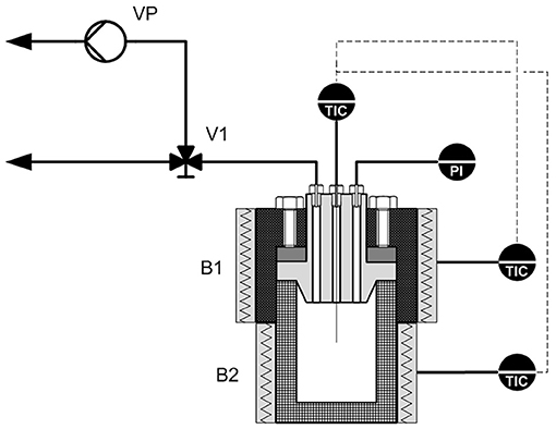
Figure 1. Schematic of the experimental set-up. B1, B2, electrical bands; PI, pressure gauge; TIC, temperature gauge; V1, three-ways valve; VP, vacuum pump.

Starch was dried in an oven at 60°C for 48 h and then sieved to 500–595 μm, fir was milled to the same size and then dried at 105°C for 48 h. The reactor, containing demineralized water and 10 g of biomass (water/biomass weight ratios: 3.5/1, 7/1, 14/1 for fir, 7/1 for starch), was sealed and evacuated. Experiments run for six different residence times (0, 10, 15, 30, 60, and 120 min), at 200°C (starch) and 250°C (fir), and under autogenous pressure (42.0 and 17.5 bar, respectively). The reactor warm-up took place at 9°C/min. The residence time of 0 means that the content was recovered at the end of the warm-up. The transient affects the conversion negligibly. The reactor end-point quenching lasted 4 min (from 200 to 150°C by in situ compressed air blowing, up to 30°C by immersion in a cold-water bath). The gas phase, mainly CO₂, was negligible, accounting for 3.5% of the dry biomass at the most. Liquid and solid products were separated by filtration, and the solid was dried at 105°C up to constant weight.

Analytical

All measurements were in triplicate, with a standard deviation of at most 4%. Hydrochar CHNS analyses (PerkinElmer-2440 series II elemental analyzer) went according to the ASTM D3176-89 standard test method for coal and coke, estimating the oxygen content by the difference (ash-free base). The liquid phase's electrical conductivity was measured with a conductivity meter (Amel Instruments 96117) using a temperature-integrate probe.

Computer Routines

All the routines were developed under the MATLAB^® platform, making extensive use of built-in functions. The programs served the purpose of this introductory and illustrative paper. More advanced, high-performance routines could derive from the basic examples directly. The interested reader could refer to comprehensive books (Tarantola, 2005; Gelman et al., 2013).

The Mersenne twister algorithm generated the necessary pseudorandom numbers. The programs ran on a standard PC without human intervention in the intermediate stages. The most demanding of the runs took 5 min of machine time to reach convergence.

Modeling

General Framework

A survey of HTC kinetics literature reveals that investigations on the residence time as an isolated parameter seldom appear. Usual approaches are to reduce model complexity by lumping time and temperature into the severity parameter and diminishing the laboratory duty with the design of experiments. However, only a comprehensive investigation of the time-course could help design the industrial process with the optimal reactor productivity. The hydrochar forms with two different stages, primary and secondary, partially overlapped and occurring at different rates (Lucian et al., 2019; Jung et al., 2020). The process exhibits two different characteristic times, and hence detailed kinetic studies should use time-data to the best of the experimental availabilities.

In the scarcity of data, the fit of complex, multi-parameter models with the traditional non-linear optimization methods could fail to locate the correct values of the kinetic constants. These iterative procedures do not guarantee per se to explore the parameter space exhaustively for reaching the global minimum of the misfit function (sum of squared errors). Moreover, the estimate of parameter uncertainty makes use of formulas derived from linear regression theory and gives approximate confidence regions. Techniques based on MCMC random walks help address these drawbacks, as already demonstrated in chemical engineering (Zhukov et al., 2015).

Another possible use of stochastic methods is the study of HTC reaction patterns. Most HTC models use mass-action kinetics networks, which lead to systems of ordinary differential equations solvable via numerical integration. Whenever the reacting population consists of large numbers of individuals, this deterministic approach gives satisfactory results. However, when considering a relatively low number of individuals, the reactions' underlying stochasticity could appear and give critical issues. This situation could well occur for biomass particles undergoing HTC so that stochastic simulation algorithms (SSA) could contribute to gain knowledge on the system dynamics and the distribution of products generated into the reactor. Statistic-based techniques imply many calculations but, nowadays, computing power is available at a relatively low cost, making massive calculation techniques accessible. The Monte Carlo methods of this study are one example of these number-crunching procedures. The programs explicitly developed for this paper demonstrate how to apply these statistical methods to HTC easily.

Programs

This study uses two different programs to perform regressions and test reaction networks, respectively referred to as programs (A) and (B).

Figure 2 is a schematic flow chart of the method adopted in program (A).

FIGURE 2

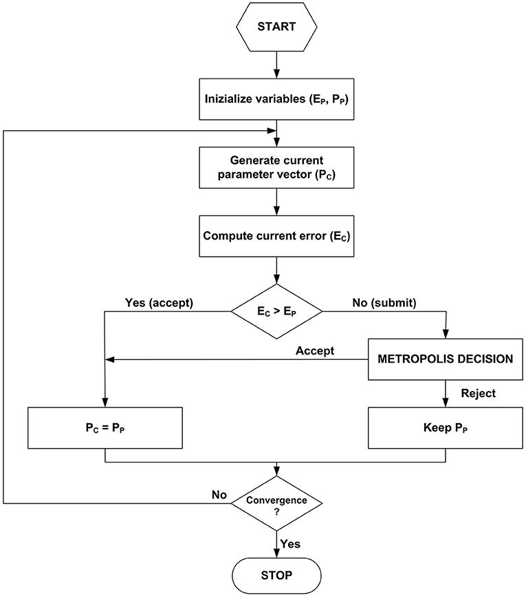
Figure 2. Schematic flowchart of program (A). See the text for details.

This routine searches for the global optimum performing a Brownian walk in the parameter space, driven by probability. The next iteration step depends only on the previous one. Hence, the process is a Markovian one. To locate the start-point, one needs a rudimentary knowledge of parameter estimates, typically coming from previous evidence or traditional fitting. Here, the start position is determined by altering each initial parameter estimates through a uniformly distributed random number. A random move is always accepted if it improves the fit, i.e., reduces the current value of the quadratic error function:

$\begin{array}{ll}{E}_c(P_c)={\displaystyle \sum }{(M(P_c)-D)}^2& (1)\end{array}$

where P_c is the current estimand vector, D the vector of depending variable observations, M the model response. The summation is over all the N experimental observations. The current values defined by Equation (1) are iteratively compared to those computed at the previous step (E_p, P_p). P_c is generated resorting to a jumping distribution. Each element of P_p receives a uniformly distributed random variation (±0.5%) in the present case. The program's core is the Metropolis decision, which accepts conditionally a fraction of moves that worsen the fit. This procedure allows the walker to escape from possible local minima and explore the surrounding portion of the space, searching for the global optimum. The acceptance check makes use of the ratio of conditional probabilities:

$\begin{array}{ll}A=\frac{p(P_C|D)}{p(P_P|D)}& (2)\end{array}$

The proper likelihood density functions p in Equation (2) are the exponentials of the errors (Tarantola, 2005). The jump is accepted if:

$\begin{array}{ll}Kexp\left[-\frac{1}{2}\left(E_c-E_p\right)\right]>r& (3)\end{array}$

where r is a uniformly distributed pseudorandom number between 0 and 1 and K a tunable scaling factor, whose correct value leads to an acceptance rate, i.e., the ratio of passed jumps to the total examined, between 25 and 35% (Gelman et al., 2013). The trial-and-error setting of K depends on the examined model and is inherent to classical Metropolis algorithms. More advanced procedures are available in the literature, not requiring the tuning. The present simplified form provides reliable results and serves well for this illustrative paper.

A good practice is to discharge the first half of the iterations (burn-in) to make the sequences less sensitive to the starting distribution. The recommended approach to assess the convergence is to compare different sequences, independent of each other and originating from different start-points. Let consider m parallel sequences of equal length n. For each scalar estimand P, the simulation draws are labeled P_{i, j} (i = 1,…, n; j = 1,…, m). The program computes B and W, the between- and within-sequence variances, respectively:

$\begin{array}{l}B=\frac{n}{m-1}{{\displaystyle \sum }}_{j=1}^m{\left({\overline{P}}_j-\stackrel{-}{\stackrel{-}{P}}\right)}^2,{\overline{P}}_j=\frac{1}{n}{{\displaystyle \sum }}_{i=1}^n{P}_{ij},\\ \stackrel{-}{\stackrel{-}{P}}=\frac{1}{m}{{\displaystyle \sum }}_{j=1}^m{\overline{P}}_j& (4)\end{array}$

$\begin{array}{ll}W=\frac{1}{m}{{\displaystyle \sum }}_{j=1}^m{s_j}^2,{s_j}^2=\frac{1}{n-1}{{\displaystyle \sum }}_{i=1}^n{\left(P_{ij}-{\overline{P}}_j\right)}^2& (5)\end{array}$

The monitoring of convergence of the iterative simulation occurs by estimating the factor by which the scale of the current distribution might reduce continuing the procedure in the limit n → ∞:

$\begin{array}{ll}\widehat{R}=\sqrt{\frac{\frac{n-1}{n}W+\frac{1}{n}B}{W}}& (6)\end{array}$

Equation (6) defines a reduction factor that tends to 1 as n → ∞. As a conservative choice, the program stops once each estimand parameter gives values <1.1. The second halves of all the sequences are collected and treated as a comprehensive sample from the target distribution. Typically, 30,000 iterations and 10 walkers were enough for an exhaustive analysis.

Figure 3 reports the schematic procedure for program (B), an elementary form of the classical Gillespie's algorithm (Erban and Chapman, 2019).

FIGURE 3

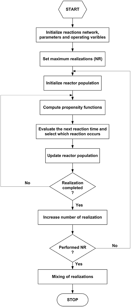
Figure 3. Schematic flowchart of program (B). See the text for details.

First, one defines the network of pseudo-reactions between the species ruling the HTC kinetics and the relative parameter values. Although this study analyzes simple, two-reactions mechanisms, more complex patterns are easily implementable. Once set the species population variables at time zero (typically, the total number of individuals equal to 100), the system evolution simulation proceeds autonomously. For each postulated reaction, the program recursively computes the propensity functions (α), i.e., the probability of a reaction to occur in the time interval (t, t+dt). The propensity is the product of the specific probability rate and the reaction degeneracy, i.e., the number of distinct interactions between reacting species. Elementary reactions give a simple formulation of the propensity. As an example, for the generic reaction between R1 and R2 to give P:

$\begin{array}{ll}\alpha =\left(\frac{k}{V}\right)R1(t)R2(t)dt& (7)\end{array}$

where R1(t) and R2(t) are the instantaneous numerosities of the two species, k the characteristic frequency of the reaction per unit volume V. According to Equation (7), all species are homogeneously distributed within the reactor. The extension to comprise heterogeneous compartments is not tricky.

In the presence of r simultaneous reactions, the total propensity α_T is simply the sum of all the individual ones:

$\begin{array}{ll}{\alpha }_T={{\displaystyle \sum }}_{i=1}^r{\alpha }_i(t)& (8)\end{array}$

The total propensity measures the system's reactivity, i.e., how likely a reaction is to occur in the infinitesimal time interval dt. The higher the propensity, the higher the rapidity of reacting system transformation. The probability that more than one reaction occurs in the time interval is an infinitesimal of higher-order and therefore negligible. The program generates the time elapsed before a reaction occurs (τ) and selects which one of the two reactions progresses through two uniformly distributed pseudo-random numbers between 0 and 1(r₁, r₂). Equation (9) computes the time of the subsequent reaction (τ) sampling from the exponential distribution:

$\begin{array}{ll}\tau =\frac{1}{{\alpha }_T}ln\left(\frac{1}{r_1}\right)& (9)\end{array}$

The instantaneous total propensity makes the reaction time to increase stochastically by unequal steps, of arbitrary units of measurement, according to the Markovian dynamics. The next reaction to take place at the current time is the first one if the following inequality verifies:

$\begin{array}{ll}{r}_2<\frac{{\alpha }_1}{{\alpha }_2}& (10)\end{array}$

In the opposite case, it is the second reaction that occurs. The discriminating inequality (10) could be generalized to consider multiple reaction networks easily. Once identified the active reaction, the program updates the species balances diminishing by one the reactants and increasing by one the products involved. The procedure iterates until a stop criterion verifies, i.e., one of the reactants drops to zero, or the time reaches the predefined maximum. The program repeats the stochastic simulations for a number NR of parallel realizations and averages across all the results to obtain the simulated time-course of all the species. From 20 to 100 realizations are enough to get a result statistically significant. The outputs of program (B) furnish a rapid detection of the system dynamics and select candidate reaction schemes like the traditional method of numerical integration of the differential equations. The examples detailed in the discussion of the results are explanatory of the procedure.

Results and Discussion

Table 1 summarizes the datasets over which the programs run and Table 2 details the results of the experiments of this study.

TABLE 1

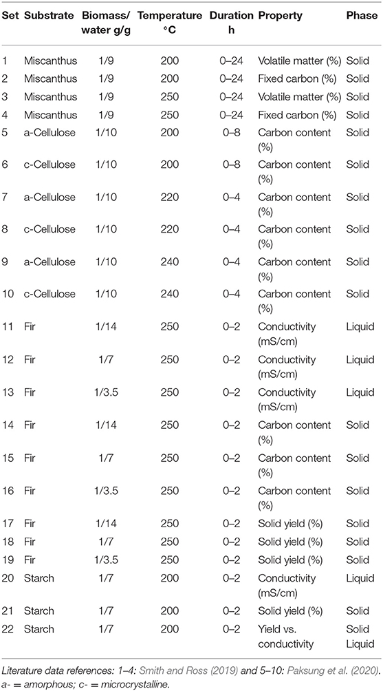
Table 1. Synopsis of the data from literature and from this study.

TABLE 2

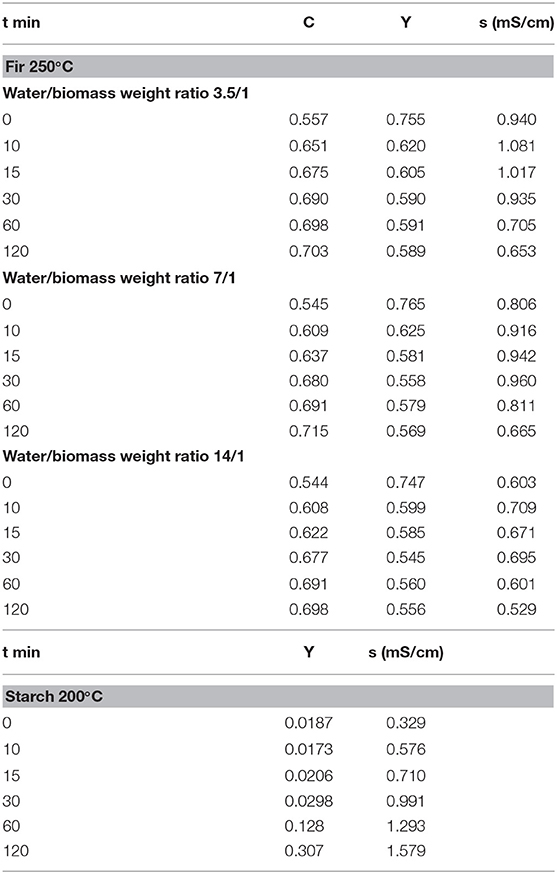
Table 2. Experimental results obtained in this study.

The datasets encompass a wide range of operational conditions and serve as a stress-test for assessing the routines' reliability. Substrates are representative of herbaceous biomass [miscanthus (Smith and Ross, 2019)], model carbohydrates [cellulose (Paksung et al., 2020)], lignocellulosic materials (fir) and agro-food industry scraps (potato starch). Temperature ranges from 200 to 250°C, reaction duration from 2 to 24 h, the solid-liquid ratio from 1:3.5 to 1:14. The programs analyzed the time course of significant properties of the hydrochar, e.g., mass yield, volatile matter, total carbon content, and fixed carbon. The liquid phase electrical conductivity was also studied as it previously proved to be a convenient lumped parameter for monitoring the reaction progress (Gallifuoco et al., 2018).

The misfit functions used two different model equations. For the data referring to the solid phase, the following logistic equation mostly proved to give the best fitting performances (Gallifuoco and Di Giacomo, 2018; Gallifuoco, 2019):

$\begin{array}{ll}M=P1+\frac{(P2-P1)}{1+{\left(\frac{t}{P3}\right)}^{P4}}& (11)\end{array}$

The time-course of liquid phase conductivity follows a series mechanism given by two first-order steps, formation plus depletion (Gallifuoco et al., 2018). Accordingly, the proper equation is:

$\begin{array}{ll}M=P1\left[1-exp(-P2t)\right]+P3exp(-P4t)& (12)\end{array}$

In both Equations (11, 12), t is the reaction time and P1…P4 the estimand parameters. In Equation (11), P3 is the time scale, P4 a shape factor, and P1 and P2 the final and the initial values, respectively. Equation (12) has two different time scales, P2 and P4. The initial value is P3, the final one P1. According to data of Table 1, the software performed 22 fittings of 4 parameters each, which sum up to 88 different estimates.

The use of model equations is an entry-level problem for illustrating the features of program (A). More advanced applications are possible, such as the inverse problem of fitting parameters to the system of ordinary differential equations coming from a hypothesized reaction network.

The misfit functions associated with Equations (9, 10) lie in the 5-dimensional space, and consequently, complete visualization of the random walks is not possible. Nevertheless, plots of any couple of parameters could illustrate the essential features. Figure 4 shows typical examples of the results and serves well in the discussion.

FIGURE 4

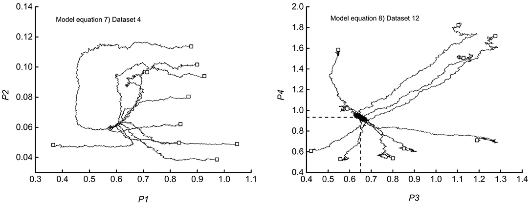
Figure 4. Examples of random walks on the space parameter.

The diagrams trace the 10 random walks from the start-point (□) to the end (♢). By way of comparison, the figure also locates the non-linear least square estimate (⋆). By inspection of the left-hand diagram, which refers to dataset 12 of Table 1, one could observe that the walkers, after the initial wandering in far, not significant regions, converge on the expected target. The right-hand diagram (dataset 4) shows more straight tracks that flow into a specific portion of the parameter plane, crowded enough to hide the endpoints. The numerical outputs show that all the walkers hit the same point, coincident with the least square estimate. The intersection of the two dashed segments locates the coordinates of the final estimate (0.647, 0.933). The trajectories in the right-hand diagram signal that the valley surrounding the minimum has steep walls. Figure 5 shows examples of the satisfactory accordance of predictions with experimental data. Figure 6 reports a selection of data vs. time plots and the fitting lines connected to the parameters' endpoint estimates.

FIGURE 5

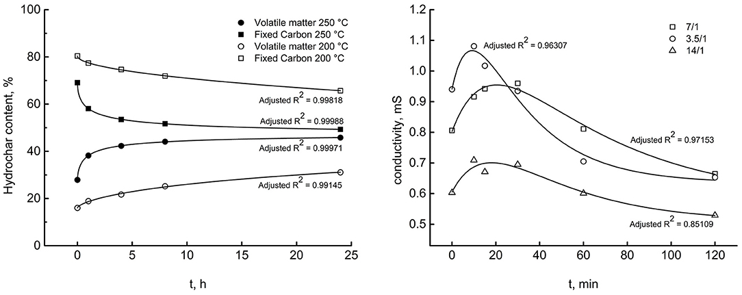
Figure 5. A selection of experimental data and regression lines estimated by program (A). Left, model Equation (11), datasets 1–4. Right, model Equation (12), datasets 11–13, effect of liquid/solid weight ratio.

FIGURE 6

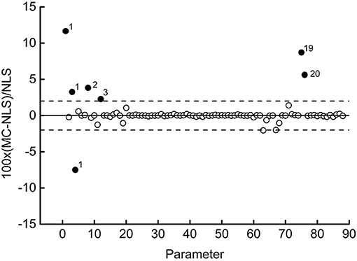
Figure 6. Synopsis of all the estimated parameters. Percent deviations between estimates: NLS, non-linear least-squares; MCMC, Markov chain Monte Carlo.

Other plots, not reported here to avoid crowding the paper, give similar results, so the discussion of Figure 6 assumes the character of generality. The adjusted R²s, shown next to the respective correlation curves, prove that the software works satisfactorily with both the model equation, whatever the HTC conditions were. The left diagram refers to Miscanthus at two reaction temperature and reports the time courses of hydrochar fixed carbon and volatile matter content. The right diagram refers to starch and records the evolution of liquid phase electrical conductivity at three different liquid/solid weight ratios.

Comparing the obtained parameter values with those coming from the traditional non-linear least-squares method (Levemberg-Marquardt algorithm) allows testing the reliability of the MCMC technique. Figure 7 summarizes the results obtained.

FIGURE 7

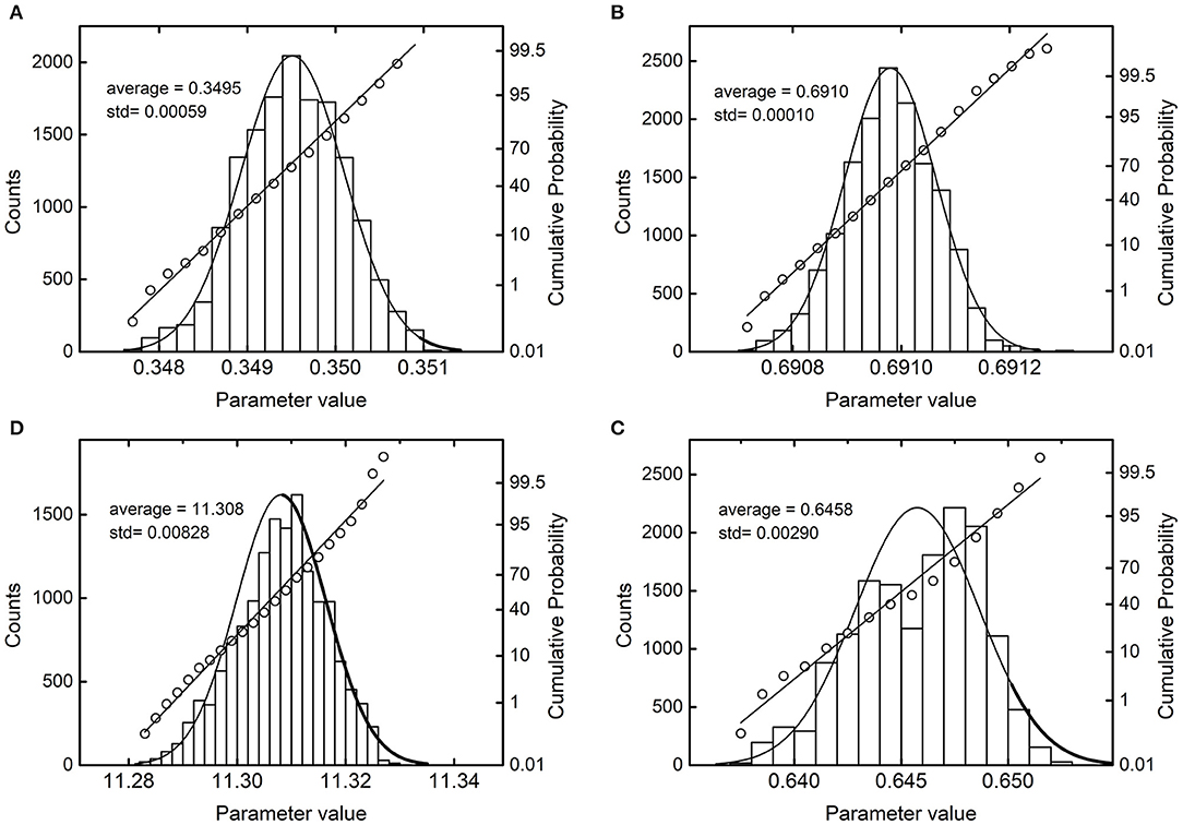
Figure 7. Probability density plots and probit plots of a selection of parameters. (A) Dataset 21, parameter P1; (B) dataset 3, parameter P2; (C) dataset 4, parameter P3; (D) dataset 10, parameter P4.

The diagram shows the relative percentage deviation between the value estimated by the program (MCMC) and that obtained with least squares (NLS) for each of the 88 parameters. Most of the points align with unity (full line), indicating substantial equality between the two estimates. Six values out of the 88 are within a ±2% deviation (dashed lines). The remaining 8 points (full symbol) deserve further discussion. The numbers to the right of symbols label the dataset to which the parameter belongs. So, three out of four parameters of dataset 1 differ significantly from the respective values obtained with the least-squares method.

Interestingly, in this case, the MCMC method found a global minimum, whose misfit function assumes a value lower than that of NLS. This circumstance also occurs for dataset 3, although to a lesser extent. Datasets 2 and 20 represent opposite cases, in which NLS performs better than MCMC. The increase of iterations above 30,000 did not improve the result, and one could conclude that these two cases deserve further investigation. A more precise diagnosis would require increasing the number of walkers to reduce the effect of individual deviations. For this study, however, one could conclude that the software passed the reliability test entirely. It can detect global minima that elude the NLS method.

NLS methods are fast algorithms for identifying the misfit function's global minimum with models of low dimension. With the increase in model dimensions, these techniques become inefficient and vulnerable to finding a local minimum closest to the starting point rather than the desired global minimum. To overcome this limit, one could repeat the optimization with various starting points and monitor if they all converge to the same solution. This stratagem is prone to become computationally expensive and troublesome as one complies with many parameters. Although this study analyzes few-parameters models, in some cases, NLS failed to find the global minimum. Changing the routine's conditioning and exploring up to 100 different starting points did not improve the performance. One could expect that the advantage of MCMC over NLS becomes even more evident with multi-parameter models. Conversely, the increase of the model complexity could make the computational cost of MCMC higher than that of traditional least-square methods. Hence, to deal with more detailed reaction schemes, one should resort to more sophisticated MCMC algorithms, well-established in the literature. It is worth overstepping the scope of this introductory study and prosecute the research in this way.

Finally, dataset 19 shows the value of one of its parameters which differs sensibly (+8.71%) from the corresponding one estimated by NLS, although the misfit function's value is substantially the same with the two methods. This last result warns not to accept any regression method ipso facto, especially when the estimated parameters are critical variables for the subsequent process design. The Bayesian paradigm considers parameters as random variables whose distributions are updated by the knowledge of experimental data. The steps after the burn-in period sample repeatedly from these distributions, and this furnishes valuable information on each parameter. Table 3 sums up all the results.

TABLE 3

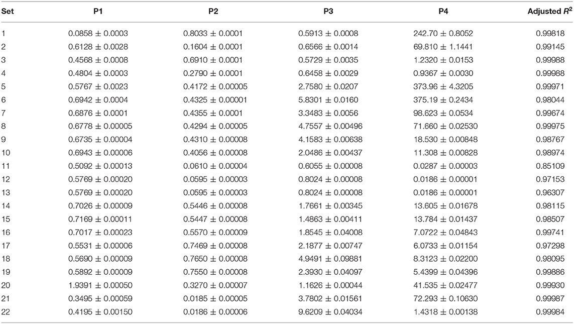
Table 3. Statistical properties of the algorithm (A) outputs.

One can observe that all the estimands deviate from the average value within a very narrow range. The satisfactory regressions of experimental data (adjusted R-square factors appear in the last column) reinforce the precision of estimates. Figure 7 visualizes the near-convergence samplings of four selected parameters and serves as an example of the general results.

For reference, each histogram shows the normal probability distribution. The probit analysis, which uses the cumulative probabilities to test the normality of the distribution, is superimposed to the histograms. The more the points align on a straight line, the more the observed distribution approximates the normal one. In Figure 7, the most significant deviations appear in C and D, where the distributions are slightly left-skewed. More in-depth elaborations are possible, although beyond the scope of this introductory study.

Program (B) run on reaction networks reported in Table 4.

TABLE 4

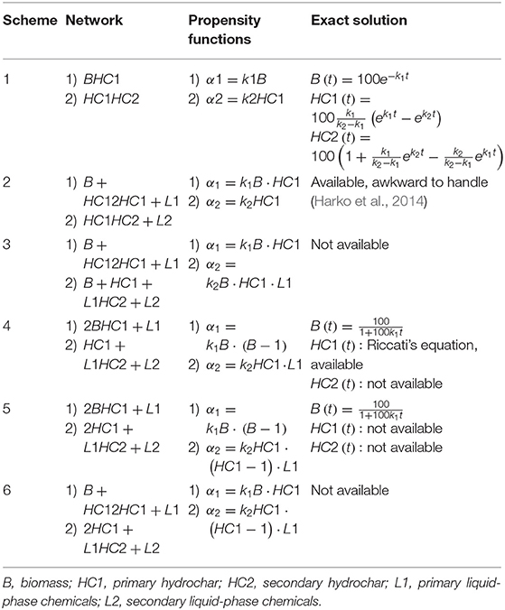
Table 4. Model networks tested with program (B).

All the schemes make use of mass-action kinetics between compartments and respect essential literature findings. As the amount of gaseous phase generated by the low-temperature hydrothermal reactions negligible, no compartment for gas species appear. Hydrochar formation is a two time-scale process, and accordingly, the networks involve two distinct pseudo-kinetic constants, k₁ and k₂. Moieties released in the liquid by primary hydrochar formation contribute to build-up secondary hydrochar, and the schemes entail liquid-phase compartments. As the reaction proceeds, the solid yield (recovered solid/biomass) should decrease, and hydrochar energy density should increase.

In the following, B stands for biomass, HC1 for primary hydrochar, HC2 for secondary hydrochar, and L1 an L2, respectively, for the corresponding liquid-phases substances. Scheme 1 is the simplest one. This naïve model, a test bench for assessing the reliability of program (B), conceives the HTC as a first-order two-step process and disregards the dynamics of liquid phases species. The related system of three ordinary differential equation has a straightforward solution, reported in Table 4. Figure 8 illustrates the results of the tests.

FIGURE 8

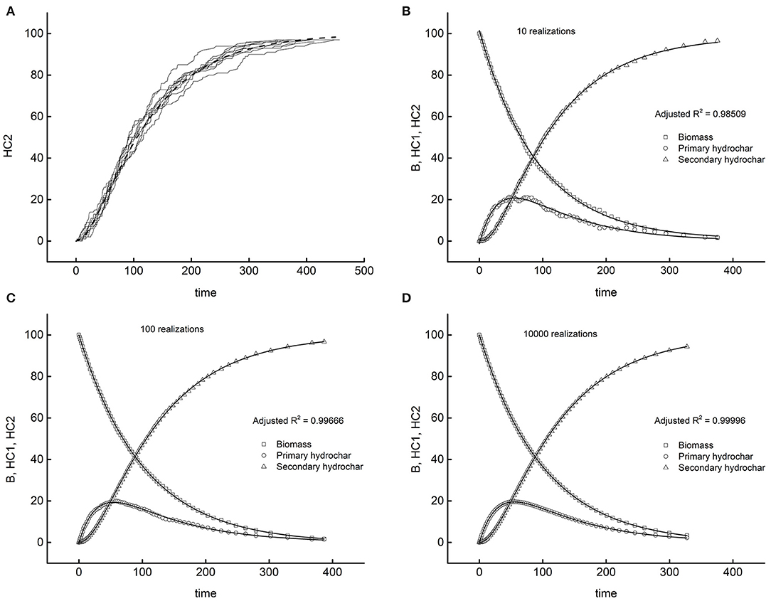
Figure 8. The test bench of program (B) with scheme 1. Dashed lines, exact solutions; symbols, simulations. (A) Ten realizations of secondary hydrochar dynamics. Remaining diagrams (B–D) averages on increasing number of realizations.

Diagram A traces 10 simulations of the dynamics of the secondary hydrochar, each originating from the same initial condition (t = 0, HC1 = HC2 = 0, B = 100). The random trajectories follow independent paths, relatively different from each other, but matching on average the exact solution (dashed line) reported in Table 4. Expectably, the more the realizations performed, the higher the precision of the results, as demonstrated by the other diagrams of the Figure. Each of them reports the averages across all realizations for the three species and the corresponding exact solutions. The number of realizations performed to simulate the system enlarges moving clockwise from the upper right diagram to the lower left one. One can easily verify that the precision of the simulations increases, as proved by the reported adjusted R-squares of the worst fitting among the three of each diagram. One could observe that 10 realizations suffice for obtaining a satisfactory average. The remaining diagrams demonstrate how the fluctuations reduce if one performs a higher number of simulations. Diagram D displays the simulation coming from 10,000 realizations, with just five seconds of computing time. It appears that program (B) correctly behaves, since the stochastic simulation tends to coincide with the exact solution in the limit of infinite realizations, and the computing task for attaining a satisfactory approximation is affordable.

The remaining schemes are worth considering as tentative, more detailed descriptions of the HTC reactions. The literature remarks on the solid-phase autocatalytic behavior of HTC (Brown, 1997; Paksung et al., 2020), and the first reaction of schemes 2, 3, and 6 accounts for this. For activating the process, a certain amount of HC1 should be present as the reactions start (time zero, reactor heated up to the setpoint temperature). Experimental evidence confirms that a partial biomass transformation occurs during the reactor warmup. The more the transient lasts, the higher the extent of modification. For example, in datasets 1–4, the per cent fixed carbon of native biomass is 12.3, those of time zero are 16.0 and 27.9, respectively, for 200–250°C (Smith and Ross, 2019). The finding is generally evident for lignocellulosic materials, as confirmed by the experiments of this study. Non-lignocellulosic biomass, such as starchy materials, could undergo the entire first step in the warmup. In eventuality, solid yields could increase with the reaction time. A cautious choice of the initial conditions could allow the simulation run in agreement with the experimental observations. The second reactions of Table 4 account for the formation of secondary hydrochar via interactions between liquid and solid phases. The schemes envisage the progressive reduction of solid-phase species, except for network 2 (solid balance of zero), which could adapt to cases of increasing solid yield. The improvement of these illustrative networks is straightforward, e.g., by considering different reactions. The present basic form serves the scope of this paper and gives remarkable results, easily comparable with the experimental data to steer the selection of the proper scheme. Figure 9 illustrates typical results.

FIGURE 9

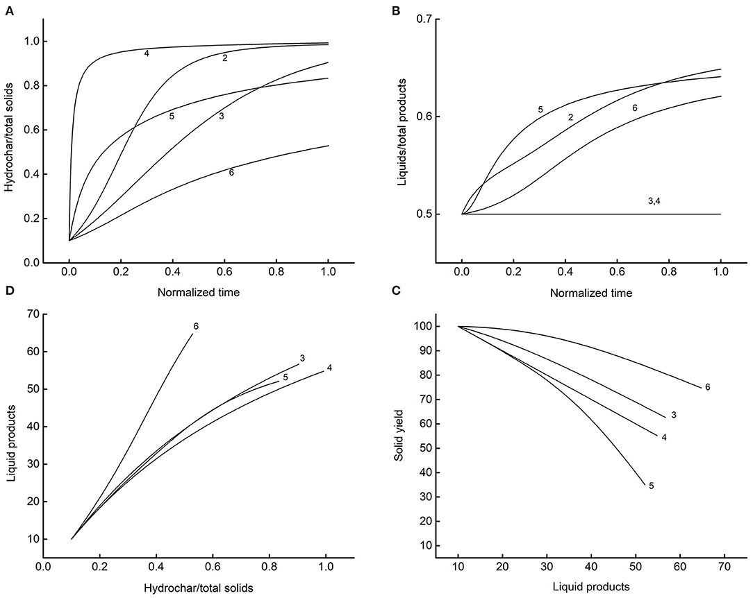
Figure 9. System dynamics associated with the reaction patterns of Table 4. The numbers next to lines label the scheme. (A) Time course of the conversion to hydrocar; (B) progression of liquid-phase moieties accumulation; (C) relationships between solid and liquid phases; (D) liquid-phase build-up as a function of solid conversion.

The simulations run on equal values of the parameters (k₁ = 20, k₂ = 1, initial HC1 = 10, initial L1 = 10). Diagram A reports the fraction of hydrochars in the solid phase as a function of the normalized reaction time (end-time equal to one). Each network displays recognizable dynamics, and this helps to link the proper model to the experimental data. Diagram B gives the corresponding distribution of the liquid to solid components. The differences between schemes persist, except for models 3 and 4, intrinsically structured to produce a constant ratio of liquid to solid products. Liquid-phase analyses, both of key components and lumped properties (Gallifuoco et al., 2018), could allow evidencing the best-fitting model. Diagram C and D show the relationships between liquid and solid phases retrievable at any time from the reactor. Definite patterns appear for all schemes in that the solid recovery decreases monotonously with the accumulation of liquid product (C), and this last gives clear trace of the conversion of biomass to hydrochar (D).

Overall, the results of Figure 9 stimulate further elaborations for comparing previsions with experiments. A detailed linking of stochastic simulations with experiments allow selecting the proper reaction network. Although the schemes of this study consider a restrict number of compartments, there are sufficient to illustrate the procedure. Figure 10 shows some examples of how to bring valuable information out of the results. Diagram A reports the fixed carbon of dataset 2 vs. the corresponding simulated property for four out of the six reaction schemes. The authors (Smith and Ross, 2019) reported the fixed carbon of the native biomass (12.3%) of the time-zero solid (16.0%), and that measured after 24 h of reaction (31.1%), reasonably due to the complete conversion. One could speculate that the fixed carbon measured at intermediate times should be due to the weighted contributes of the biomass not yet reacted and the hydrochar already produced.

FIGURE 10

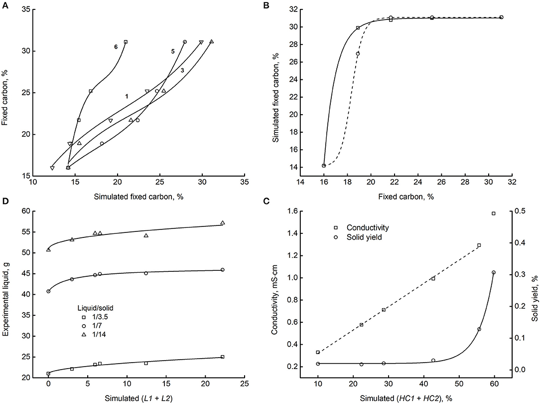
Figure 10. The matching of experiments with simulations. (A) Fixed carbon measured in dataset 2 as a function of the corresponding quantity for some reaction schemes. The numbers to the left of regression lines label the scheme. (B) Simulated vs. measured fixed carbon for scheme 2 (dashed line) and 4 (solid line). (C) Conductivity (left y-axis) and solid yield (right y-axis) of dataset 20 and 21 vs. the simulation of scheme 3. (D) Amount of liquid phase recovered by the reactor as a function of the corresponding simulation compartments. Datasets: 11, 12, and 13. Reaction scheme 6.

Similarly, the x-axis values weigh the amounts of B and (HC1 + HC2) with the experimental data. The diagram shows that the simulations match the experiments unambiguously. By the way, data fit very well third-degree polynomials (lines). Further investigation could disclose the essence of this finding and assess the possible theoretical foundations. Diagram B is analougus and refers to schemes 2 and 4. Although in these last cases, the polynomial fitting failed, ordered patterns appear connecting simulations and data unambiguously, as shown by the lines connecting points. Part C reports the direct relationship between datasets 20 and 21 and the simulated total hydrochar of reaction scheme 3. The left y-axis reports the liquid phase electrical conductivity, the right y-axis the solid yield. The solid line connecting the yields is an exponential which fits satisfactory the data (R² = 0.99919). The dashed line is a linear correlation (R² = 0.99876) of the conductivities, excluding the point on the upper right corner. Diagram C shows satisfactory matching trends and demonstrates that scheme 3 is predictive of the datasets analyzed. Finally, diagram D shows a good coupling of the amount of liquid recovered after the reaction and the corresponding compartments. Data refer to datasets 11, 12, and 13 as matched to model 6.

Figure 10 shows some of the many ways of linking experiments with simulations. One could envisage further fruitful implementations for steering the process of model assessments, obtaining at the same time valuable feedbacks on which part of the experimental investigation to strengthen. A more in-depth analysis requires identifying and quantifying liquid-phase key chemicals to match with the compartments of models. Experimental data on the dynamics of such compounds appear in the HTC literature seldom. As available, this evidence could contribute to more accurate validations.

The state-of-art on HTC kinetic modeling shows the success of both lumping and detailed descriptions of reaction networks. Models that describe the overall biomass conversion catch the autocatalytic progression of the condensed phase transformation satisfactorily (Pecchi et al., 2020). Mechanistic descriptions, involving up to a 10th of reactions and chemically defined liquid-phase products, result in a broader knowledge of the kinetic constants (Jung et al., 2020). This paper demonstrates that compartmental modeling, a sort of intermediate approach, could find room in the HTC kinetic studies. The research is proceeding this way.

Conclusions

The study demonstrates the usefulness of Bayesian statistics and Monte Carlo methods for studying biomass hydrothermal carbonization kinetics. Stochastic simulation of HTC reactions is a flexible tool for testing hypothesized networks and could improve the knowledge of the mechanism of biomass conversion. The approach could face the limit of computational expensiveness when extended to a thorough description of the reaction kinetics. The matter deserves future researches. Despite the basicity of the routines, the results are satisfactory. The estimation of the parameters furnishes regression coefficients as high as 0.9999 and detects the global minimum of the space parameters for all the datasets. The test of possible reaction schemes is straightforward. The upgrading to more sophisticated and efficient algorithms is clear-cut. It could exploit the vast library of software, readily available and long used in other areas of kinetics applied to chemical engineering. The proposed method has the potential to guide the selection of the correct kinetic model. It can flexibly simulate the dynamics of any experimentally measured property in both the solid and liquid phases.

Data Availability Statement

The original contributions presented in the study are included in the article/supplementary material, further inquiries can be directed to the corresponding author.

Author Contributions

AG conceived the work, developed the modelling, and the computers routines. AP and LT contributed equally in carrying out the experiments. All authors contributed to the article and approved the submitted version.

Conflict of Interest

The authors declare that the research was conducted in the absence of any commercial or financial relationships that could be construed as a potential conflict of interest.

References

Antero, R. V. P., Alves, A. C. F., de Oliveira, S. B., Ojala, S. A., and Brum, S. S. (2020). Challenges and alternatives for the adequacy of hydrothermal carbonization of lignocellulosic biomass in cleaner production systems: a review. J. Clean. Prod. 252:119899. doi: 10.1016/j.jclepro.2019.119899

CrossRef Full Text | Google Scholar

Avraamidou, S., Baratsas, S. G., Tian, Y., and Pistikopoulos, E. N. (2020). Circular economy - a challenge and an opportunity for Process Systems Engineering. Comput. Chem. Eng. 133:106629. doi: 10.1016/j.compchemeng.2019.106629

CrossRef Full Text | Google Scholar

Beers, K. J. (2006). Numerical Methods for Chemical Engineering. Cambridge: Cambridge University Press. doi: 10.1017/CBO9780511812194

CrossRef Full Text | Google Scholar

Brown, M. E. (1997). The Prout-Tompkins rate equation in solid-state kinetics. Thermochim. Acta 300, 93–106. doi: 10.1016/S0040-6031(96)03119-X

CrossRef Full Text | Google Scholar

Clark, J. H., Farmer, T. J., Herrero-Davila, L., and Sherwood, J. (2016). Circular economy design considerations for research and process development in the chemical sciences. Green Chem. 18, 3914–3934. doi: 10.1002/chin.201636255

CrossRef Full Text | Google Scholar

Dhaundiyal, A., Singh, S. B., Atsu, D., and Dhaundiyal, R. (2019). Application of Monte Carlo simulation for energy modeling. ACS Omega 4, 4984–4990. doi: 10.1021/acsomega.8b03442

CrossRef Full Text | Google Scholar

Erban, R., and Chapman, S. J. (2019). Stochastic Modelling of Reaction–Diffusion Processes. Cambridge: Cambridge University Press. doi: 10.1017/9781108628389

CrossRef Full Text | Google Scholar

Gallifuoco, A. (2019). A new approach to kinetic modeling of biomass hydrothermal carbonization. ACS Sustain. Chem. Eng. 7, 13073–13080. doi: 10.1021/acssuschemeng.9b02191

CrossRef Full Text | Google Scholar

Gallifuoco, A., and Di Giacomo, G. (2018). Novel kinetic studies on biomass hydrothermal carbonization. Bioresour. Technol. 266, 189–193. doi: 10.1016/j.biortech.2018.06.087

PubMed Abstract | CrossRef Full Text | Google Scholar

Gallifuoco, A., Taglieri, L., and Papa, A. A. (2020). Hydrothermal carbonization of waste biomass to fuel: a novel technique for analyzing experimental data. Renew. Energy 149, 1254–1260. doi: 10.1016/j.renene.2019.10.121

CrossRef Full Text | Google Scholar

Gallifuoco, A., Taglieri, L., Scimia, F., Papa, A. A., and Di Giacomo, G. (2017). Hydrothermal carbonization of Biomass: new experimental procedures for improving the industrial Processes. Bioresour. Technol. 244, 160–165. doi: 10.1016/j.biortech.2017.07.114

PubMed Abstract | CrossRef Full Text | Google Scholar

Gallifuoco, A., Taglieri, L., Scimia, F., Papa, A. A., and Di Giacomo, G. (2018). Hydrothermal conversions of waste biomass: assessment of kinetic models using liquid-phase electrical conductivity measurements. Waste Manag. 77, 586–592. doi: 10.1016/j.wasman.2018.05.033

PubMed Abstract | CrossRef Full Text | Google Scholar

Gelman, A., Carlin, J. B., Stern, H. S., Dunson, D. B., Vehtari, A., and Rubin, D. B. (2013). Bayesian Data Analysis, Bayesian Data Analysis. London: Chapman and Hall/CRC. doi: 10.1201/b16018

CrossRef Full Text | Google Scholar

Guo, Z., Yan, N., and Lapkin, A. A. (2019). Towards circular economy: integration of bio-waste into chemical supply chain. Curr. Opin. Chem. Eng. 26, 148–156. doi: 10.1016/j.coche.2019.09.010

CrossRef Full Text | Google Scholar

Harko, T., Lobo, F. S. N., and Mak, M. K. (2014). Exact analytical solutions of the Susceptible-Infected-Recovered (SIR) epidemic model and of the SIR model with equal death and birth rates. Appl. Math. Comput. 236, 184–194. doi: 10.1016/j.amc.2014.03.030

CrossRef Full Text | Google Scholar

Heidari, M., Dutta, A., Acharya, B., and Mahmud, S. (2018). A review of the current knowledge and challenges of hydrothermal carbonization for biomass conversion. J. Energy Inst. 92, 1779–1799. doi: 10.1016/j.joei.2018.12.003

CrossRef Full Text | Google Scholar

Ischia, G., and Fiori, L. (2020). Hydrothermal carbonization of organic waste and biomass: a review on process, reactor, and plant modeling. Waste Biomass Valor. doi: 10.1007/s12649-020-01255-3. [Epub ahead of print].

CrossRef Full Text | Google Scholar

Jung, D., Körner, P., and Kruse, A. (2020). Calculating the reaction order and activation energy for the hydrothermal carbonization of fructose. Chemie Ing. Tech. 92, 692–700. doi: 10.1002/cite.201900093

CrossRef Full Text | Google Scholar

Kruse, A., and Dahmen, N. (2018). Hydrothermal biomass conversion: Quo vadis? J. Supercrit. Fluids 134, 114–123. doi: 10.1016/j.supflu.2017.12.035

CrossRef Full Text | Google Scholar

Larragoiti-Kuri, J., Rivera-Toledo, M., Cocho-Roldán, J., Maldonado-Ruiz Esparza, K., Le Borgne, S., and Pedraza-Segura, L. (2017). Convenient product distribution for a lignocellulosic biorefinery: optimization through sustainable indexes. Ind. Eng. Chem. Res. 56, 11388–11397. doi: 10.1021/acs.iecr.7b02101

CrossRef Full Text | Google Scholar

Lee, S. Y., Sankaran, R., Chew, K. W., Tan, C. H., Krishnamoorthy, R., Chu, D.-T., et al. (2019). Waste to bioenergy: a review on the recent conversion technologies. BMC Energy 1:4. doi: 10.1186/s42500-019-0004-7

CrossRef Full Text

Li, L., Flora, J. R. V., and Berge, N. D. (2020). Predictions of energy recovery from hydrochar generated from the hydrothermal carbonization of organic wastes. Renew. Energy 145, 1883–1889. doi: 10.1016/j.renene.2019.07.103

CrossRef Full Text | Google Scholar

Lucian, M., Volpe, M., and Fiori, L. (2019). Hydrothermal carbonization kinetics of lignocellulosic agro-wastes: experimental data and modeling. Energies 12:516. doi: 10.3390/en12030516

CrossRef Full Text | Google Scholar

Murele, O. C., Zulkafli, N. I., Kopanos, G., Hart, P., and Hanak, D. P. (2020). Integrating biomass into energy supply chain networks. J. Clean. Prod. 248:119246. doi: 10.1016/j.jclepro.2019.119246

CrossRef Full Text | Google Scholar

Paksung, N., Pfersich, J., Arauzo, P. J., Jung, D., and Kruse, A. (2020). Structural effects of cellulose on hydrolysis and carbonization behavior during hydrothermal treatment. ACS Omega 5, 12210–12223. doi: 10.1021/acsomega.0c00737

PubMed Abstract | CrossRef Full Text | Google Scholar

Pecchi, M., Patuzzi, F., Benedetti, V., Di Maggio, R., and Baratieri, M. (2020). Kinetic analysis of hydrothermal carbonization using high-pressure differential scanning calorimetry applied to biomass. Appl. Energy 265:114810. doi: 10.1016/j.apenergy.2020.114810

CrossRef Full Text | Google Scholar

Román, S., Ledesma, B., Álvarez, A., Coronella, C., and Qaramaleki, S. V. (2020). Suitability of hydrothermal carbonization to convert water hyacinth to added-value products. Renew. Energy 146, 1649–1658. doi: 10.1016/j.renene.2019.07.157

CrossRef Full Text | Google Scholar

Safarian, S., Unnþórsson, R., and Richter, C. (2019). A review of biomass gasification modelling. Renew. Sustain. Energy Rev. 110, 378–391. doi: 10.1016/j.rser.2019.05.003

CrossRef Full Text | Google Scholar

Sherwood, J. (2020). The significance of biomass in a circular economy. Bioresour. Technol. 300:122755. doi: 10.1016/j.biortech.2020.122755

CrossRef Full Text | Google Scholar

Shields, B. J., Stevens, J., Li, J., Parasram, M., Damani, F., Martinez Alvarado, J. I., et al. (2021). Bayesian reaction optimization as a tool for chemical synthesis. Nature 590, 89–96. doi: 10.1038/s41586-021-03213-y

PubMed Abstract | CrossRef Full Text | Google Scholar

Smith, A. M., and Ross, A. B. (2019). The influence of residence time during hydrothermal carbonisation of miscanthus on bio-coal combustion chemistry. Energies 12:523. doi: 10.3390/en12030523

CrossRef Full Text | Google Scholar

Tarantola, A. (2005). Inverse Problem Theory and Methods for Model Parameter Estimation, Inverse Problem Theory and Methods for Model Parameter Estimation. Philadelphia, PA: Society for Industrial and Applied Mathematics. doi: 10.1137/1.9780898717921

CrossRef Full Text | Google Scholar

Terrell, E., Dellon, L. D., Dufour, A., Bartolomei, E., Broadbelt, L. J., and Garcia-Perez, M. (2020). A review on lignin liquefaction: advanced characterization of structure and Microkinetic modeling. Ind. Eng. Chem. Res. 59, 526–555. doi: 10.1021/acs.iecr.9b05744

CrossRef Full Text | Google Scholar

Tula, A. K., Eden, M. R., and Gani, R. (2020). Computer-aided process intensification: challenges, trends and opportunities. AIChE J. 66:e16819. doi: 10.1002/aic.16819

CrossRef Full Text | Google Scholar

Ubando, A. T., Felix, C. B., and Chen, W. H. (2020). Biorefineries in circular bioeconomy: a comprehensive review. Bioresour. Technol. 299:122585. doi: 10.1016/j.biortech.2019.122585

PubMed Abstract | CrossRef Full Text | Google Scholar

Usman, M., Chen, H., Chen, K., Ren, S., Clark, J. H., Fan, J., et al. (2019). Characterization and utilization of aqueous products from hydrothermal conversion of biomass for bio-oil and hydro-char production: a review. Green Chem. 21, 1553–1572. doi: 10.1039/C8GC03957G

CrossRef Full Text | Google Scholar

Weber, K., Li, T., Løvås, T., Perlman, C., Seidel, L., and Mauss, F. (2017). Stochastic reactor modeling of biomass pyrolysis and gasification. J. Anal. Appl. Pyrolysis 124, 592–601. doi: 10.1016/j.jaap.2017.01.003

CrossRef Full Text | Google Scholar

Zhan, L., Jiang, L., Zhang, Y., Gao, B., and Xu, Z. (2020). Reduction, detoxification and recycling of solid waste by hydrothermal technology: a review. Chem. Eng. J. 390:124651. doi: 10.1016/j.cej.2020.124651

CrossRef Full Text | Google Scholar

Zhukov, V. V., Laari, A., and Koiranen, T. (2015). Kinetic modeling of high-pressure pyrite oxidation with parameter estimation and reliability analysis using the Markov Chain Monte Carlo Method. Ind. Eng. Chem. Res. 54, 9920–9930. doi: 10.1021/acs.iecr.5b02374

CrossRef Full Text | Google Scholar