 Vincenzo Russo
 Henrik Grénman
 Tommaso Cogliano
 Riccardo Tesser
 Tapio Salmi
- 1Department of Chemical Sciences, University of Naples Federico II, Naples, Italy
- 2Laboratory of Industrial Chemistry and Reaction Engineering, Åbo Akademi University, Turku, Finland
In the present work, the extended shrinking film model (ESFM) was applied to a reversible reaction in which a solid dissolves and reacts with a component present in the liquid phase. The model considers the reactive solid dissolution in the liquid phase and the diminishing of its radius with the reaction time. Furthermore, the liquid film surrounding the particle, through which the liquid component diffuses to react with the dissolved solid, is considered radius dependent; thus, the model is based on the mass balance equations derived for the solid surface, liquid bulk, and the liquid film. The model consists of two ODEs and a PDE, solved numerically with gPROMS ModelBuilder 4.0. It was demonstrated that the model can cover a wide range of operation conditions, and it shows a high degree of flexibility, allowing the application to several kinds of solid-fluid processes, such as esterification, gasification, and steam cleaning for the removal of dangerous and polluting gases (CO2, SO2) from the main process stream and NO capture.
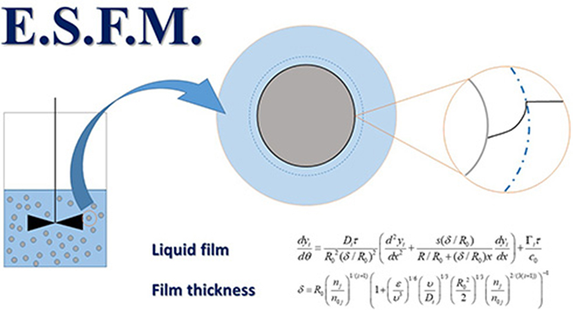
Graphical Abstract. Extended Shrinking Film Model (E.S.F.M.) for fluid-solid systems.
Highlights
- Application of the extended shrinking film model (ESFM)
- Liquid-solid reversible reaction as a case study
- Non-reactive system was simulated
- Film thickness variation along with time and particle radius
- Non ideal particles surface was considered
- General model equations for the application on different solid shapes.
Introduction
In the chemical industry, a lot of solid-fluid processes of high importance are applied, such as reduction of iron oxides, combustion of solid fuels, gasification of coal, and removal of pollutants. Moreover, more solid-fluid systems appear nowadays in chemical reaction engineering, due to the increasing use of biomass technology. The general approach for heterogeneous reactions, more specific for solid-fluid reactions, is based on the porosity of the solid. The reaction system, which considers a non-porous reactant, present fewer steps than a reaction system with a porous one. In the former case, the intraparticle diffusion is avoided, and the reaction system presents the diffusion of the component through the film because the external solid surface is present. When the chemical reaction rate is rapid, the diffusion is the rate-limiting step, so a one-step reaction system is present. Furthermore, the film thickness transfer between the phases is considered constant during the overall process as it is related to the mass and diffusion coefficients and calculated through the dimensionless Sherwood number (Sherwood et al., 1975). Customarily, the analysis of the reactions with negligible porosity, under isothermal conditions has been based on the shrinking core model (Levenspiel, 1972). Most kinetic models existing in literature to describe the solid-fluid reactions (Gibilaro et al., 1970; Williams et al., 1972; Park and Levenspiel, 1975; Jidaspow et al., 1976; Fan et al., 1977; Verbaan and Crundwell, 1986; Box and Prosser, 1989) are based on gas-solid heterogenous reactions. About the application of a reactive solid inside liquid media, few articles are present in literature with the application of the above-mentioned kinetic model (Lindman and Simonsson, 1979; Ranjan Jena et al., 2003). Moreover, some of them present simplifications on the kinetic model as negligible diffusion resistance toward the particle or the simple application of the film theory (Le Coenta et al., 2003). The present article is aimed to enhance the application of the film theory on solid-liquid reaction system with a non-porous solid reactant through the application of the extended film shrinking model (EFSM). The substantial difference compared to the simpler film theory is the film thickness dependence on the radial coordinate of the particle (Green and Perry, 2007), which shrinks during the reaction. The physical steps involved during the reaction of a solid immersed in a liquid are (1) partial dissolution of the solid component at the solid surface; (2) diffusion of the liquid component from the bulk toward the solid surface through the film surrounding the particle; and (3) chemical reaction in the liquid film and liquid bulk. Starting from the identification and consideration of the physical steps, the model was set up through mass balances for each phase involved in the reaction with the aim to applicate the present model to various reaction systems as demonstrated in our previous work (Russo et al., 2017; Salmi et al., 2017).
Model Development
Extended Shrinking Film Model (ESFM)
The ESFM is based on the following hypotheses (Figure 1):
• A non-porous solid reactant dissolves and reacts with the compounds presents in the liquid phase.
• The reaction takes place simultaneously in the film surrounding the particle, and in the bulk phase, the faster the reaction is, the more dominant the film reaction becomes.
• The film surrounding the particle is particle radius dependent (t2 > t1 > 0), indeed, the smaller the radius becomes as reaction proceeds, the thinner the film is (δ).
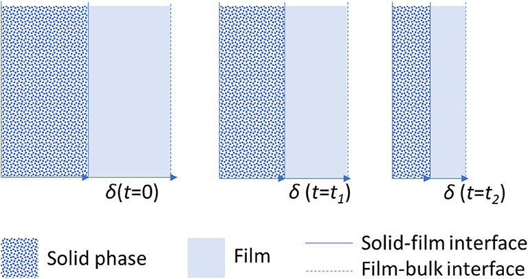
Figure 1. Solid-liquid reaction system: evolution with time of the shrinking solid and shrinking film.
However, the film thickness depends not only on the particle radius but a contribution by the degree of mixing of the reaction system is considered, too. As it is well-known, the thickness of the stagnant liquid film around the solid particle diminishes as the stirring rate of the system is increased, leading to the decrease of the particle radius due to the consumption of the solid reactant, thus to a more dominant bulk-phase reaction. These conditions are achievable in laboratory-scale experiments, in which a high stirring efficiency is easily materialized. In the industrial scale, however, it is not always possible to reach diffusion-free conditions in the treatment of dissolving solid materials when liquids and film reactions become prevailing. During the reaction, the particle dissolves reducing its radius symmetrically, however, different solid particle shapes can be considered, such as spheres, cylinders, slabs, or realistic more irregular particle geometries. No reaction inside the particle occurs as either the solid is considered non-porous or the reactions sufficiently fast to avoid any diffusion resistance inside the particle. Furthermore, for the sake of simplicity, solid particles of equal size and isothermal conditions are considered. Evidently, a more rigorous approach could consider both particle size distribution and energy balance equations. The reaction system is simulated in a batch reactor with ideal mixing, thus allowing to apply uniform concentrations into the liquid bulk phase excluding local deviations in the system. To set up the model, the mass balance needs to be written into the different zones of the system in which the reaction takes place. As discussed above, after the solid dissolution the reaction occurs only into the liquid film surrounding the particle and into the bulk of the liquid phase, so three zones need to be accounted for the mass balance, these are the solid surface, the liquid film, and the bulk of the liquid phase. Dimensionless equations were derived to express the fundamental relations between the quantities appearing in the model and to perform the numerical computations in a rational way. In the model we have a couple of ordinary differential equations (ODEs), which are the dimensionless concentrations in the liquid bulk (17) and the dimensionless amount of the solid substance (23). Additionally, partial differential equations (PDEs) are included that represent the dimensionless profiles in the liquid film (5). The latter is solved by choosing a second-order centered finite difference formula for the spatial derivatives (the number of discretization points was 40) to convert the PDEs to ODEs. The model equations were solved numerically by using the advanced modeling tool gPROMS Model Builder v.4 software (Russo et al., 2015a,b).
A little reminder about the derivatization of the equations used in the model are reported below; for more details, see our previous work (Salmi et al., 2017).
Liquid Film: Mass Balances and Film Thickness
Considering an infinitesimal control volume inside the liquid film, between the solid surface and the liquid bulk, the mass balance for a dissolved component (i) can be written as:
where Ni denotes the molar flux, A is the surface through which the components diffuse, Γi is the generation rate in the case of a single chemical reaction, and ΔV is the volume of element. For more details, see the list of symbols.
The difference between the diffusion fluxes is Δ(NiA), the amount of substances (ni) is equal to ciΔV. The volume element ΔV in Equation 1 is let to shrink (ΔV → 0), and Equation 2 is obtained after straightforward mathematical substitutions:
Equation 2 is presented in a very general form, where the shape factor (s) allows the application on different kinds of particle shapes. The shape factor s = 2 corresponds to a spherical particle, s = 1 a long cylinder, and s = 0 is a slab. For a real particle with a non-ideal surface, the shape factors can have non-integer values even exceeding 2 (Salmi et al., 2010). The non-ideality of the surface is typically assigned to surface aspects, such as cracks and craters as well as to limited porosity.
Fick's law is applied to describe the molar flux (Ni), and after developing the derivative in Equation 2, the mass balance become:
The radial coordinate changes between the value r = R on the solid surface to r = R + δ at the interphase between the liquid film and the liquid bulk.
The generation rates (Γi) are expressed by a standard stoichiometric approach:
where R denotes the reaction rate, νi is the stoichiometric coefficient of component i in the reaction.
Dimensionless film coordinate [x = (r-R)/δ)], concentration (yi = ci/c0) and time (θ = t/τ) are introduced, where δ is the film thickness, c0 the initial concentration, and τ an arbitrary reaction time. The mass balance equation for a component i in the film becomes:
where Di τ/R02 is the first dimensionless number defined (AD1), representing the extent of the molecular diffusion compared to the initial particle radius.
The following boundary conditions are needed to solve the PDE:
• x = 0: yi = (saturation of the solid components at the surface)
• x = 0: ∂yi/∂x = 0 (liquid-phase component at the surface)
• x = 1: yi = yi' (bulk-phase conditions valid at the end of the film)
According the to the film theory, the film thickness is δ = Di/kLi. It is calculated by using the standard correlation relating the Sherwood number (Sh) to the Reynolds (Re) and Schmidt (Sc) numbers (Wakao, 1984). The application to a stirred tank allows an estimation of the Reynolds number with the Kolmogorov correlation (Temkin, 1977).
The following equation was derived for the film thickness (δ) (Salmi et al., 2017):
Some considerations based on the amount of substance present into the reaction system can adapt the equations into a form better suited to practical calculations. Considering a generic instant of time, the amount of substance is nj = nP ρPVP/MP, where nP is the total number of particles in the system. Similarly, the initial amount of substance is n0j = nPρPV0P/MP. For a general geometry VP/V0P = (R/R0)s + 1. Finally, the relationship between the particle radius and the amount of substance is obtained,
Inserting the relationship into the expression for film thickness in Equation 6, the following equation is obtained:
Equation 8 reveals that the film thickness diminishes from the initial value to zero as the solid reactant (j) is consumed. The film thickness for a fixed chemical system can be diminished by stirring: with increasing the stirring speed, the energy dissipated per time (ε) increases and the film thickness decreases according to Equation 8.
The ratio R/R0 is obtained from Equation 7
A dimensionless film thickness is defined as follows:
which can be compressed defining a dimensionless number (AD2 = α) including both physical parameters and the dissipated energy of the stirring device:
Bulk-Phase Balances
The mass balance of the dissolved component (i) in the liquid bulk phase can be written as
The liquid volume (VL) is assumed to remain constant as declared above. After division by the liquid volume we obtain:
where aP represents the total outer particle surface area-to-liquid volume ratio, and it is expressed as AP/VL. For a general geometry aP/a0P = (R/R0)s.
The balance equation becomes now
After inserting the relationship between the amount of substance and the radius in Equation 7, the balance equation becomes:
The flux at the film-bulk interface is calculated from.
Finally, introducing dimensionless concentration and time, the liquid bulk balance equation is transformed to a dimensionless form:
where Dia0τ/R0 is the third dimensionless number (AD3), meaning the ratio between the diffusivity of the component weighted by the specific surface area and the initial radius of the particle. As revealed, AD1 and AD3 are related to each other as function of similar quantities.
The flux at the film-bulk interface is calculated from
Solid-Phase Balances
The mass balance equation for a solid phase component (j) is given by
where Nj denotes the diffusion flux at the dimensionless coordinate x = 0, that is, at the outer surface of the particle. The total outer surface area is A = aVL = a0 (R/R0)sVL as discussed above. The Fick's law gives the flux, which in this case becomes
The balance equation for a general particle geometry can be written as:
After inserting the relationship between the amount of substance and the radius in Equation 7, the liquid bulk balance is obtained:
The solid-phase balance equation is transformed to a dimensionless form by introducing the dimensionless time:
where c0VL/n0j is the fourth dimensionless number (AD4).
Contribution Analysis and Modeling Approach
The contribution analysis of each phase allows to know in which extent the reaction is proceeds either in the film or in the bulk phase. The contribution of the film and bulk phases to the process is evaluated calculating the instantaneous contributions of each reactions in the film and in the bulk phase, respectively. The time to the shift between the film to the bulk-dominant reaction (tshift) is measured as the inflection point of the relative contribution analysis of both film and bulk phases.
The relative contributions of the film (F) and bulk (B) for the reaction can be calculated from the following equations:
a more detailed derivation of Equations 24 and 25 is reported by Salmi et al. (2017).
As a summary, the model to be implemented consists of Equations 5, 11, 17, and 23. The set of ordinary and partial differential equations constituting the model were solved numerically using gPROMS ModelBuilder v. 4.0 software, discretizing the film thickness with a second-order centered finite difference approach, adopting 50 points of discretization grid.
Results and Discussion
In the present article the model was applied, first, to an elementary and reversible homogeneous reaction, in which a solid component B, dispersed into a liquid, dissolves, and then reacts with a component (A) present in the liquid phase. The reaction scheme is summarized below:
1. B(s) → B Dissolution
2. A + B ↔ C Reaction
As the reaction occurs in both bulk and film phases, it is necessary to define the reaction rate expressions in each phase:
For the reaction, a simple second-order reversible rate expression was adopted in which the term (ci) and (ci') are the concentration of the i-specie referred to the liquid film and the liquid bulk, respectively.
The model was applied on several reaction conditions investigating the influence of either the operation conditions or the physical parameters on the behavior of the system. Table 1 shows the parameters used in each simulation; the shape factor (s) was set equal to 3 to simulate a realistic solid particle. In addition, to calculate a0, the molar mass of the solid was fixed to 0.1 kg/mol and the solid density to 2,000 kg/m3.
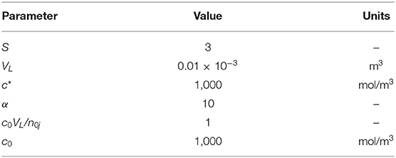
Table 1. Parameters used for the simulations.
The characteristic time, needed to make our calculation time dimensionless, was chosen arbitrarily to be τ = 1s. Due to the high number of simulations (about 60) Table 2 shows the parameters ranges adopted in the numerical simulation tests.
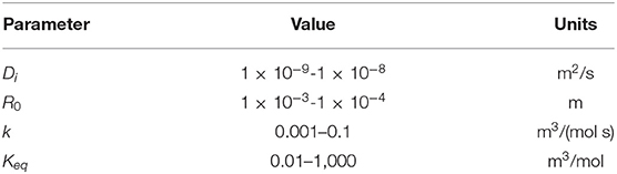
Table 2. Range adopted for each parameter selected for the sensitivity study.
Figure 2 shows the trend of the dissolution time (tdis) against the kinetics and equilibrium constant at different value of the first dimensionless number. The white zones indicate areas of the space of parameters not investigated. The absolute value of the dissolution time changes with the dimensionless number, passing from hundreds of seconds (AD1 = 1 × 10⁻³) to just 1 s (AD1 = 1). In general, as AD1 is a function of both Di and R0, an increase in AD1 value can be justified by either a higher molecular diffusivity or a lower particle radius. In both cases, the diffusion resistances become less influential, leading to a decrease of the dissolution time, as revealed in Figure 2.
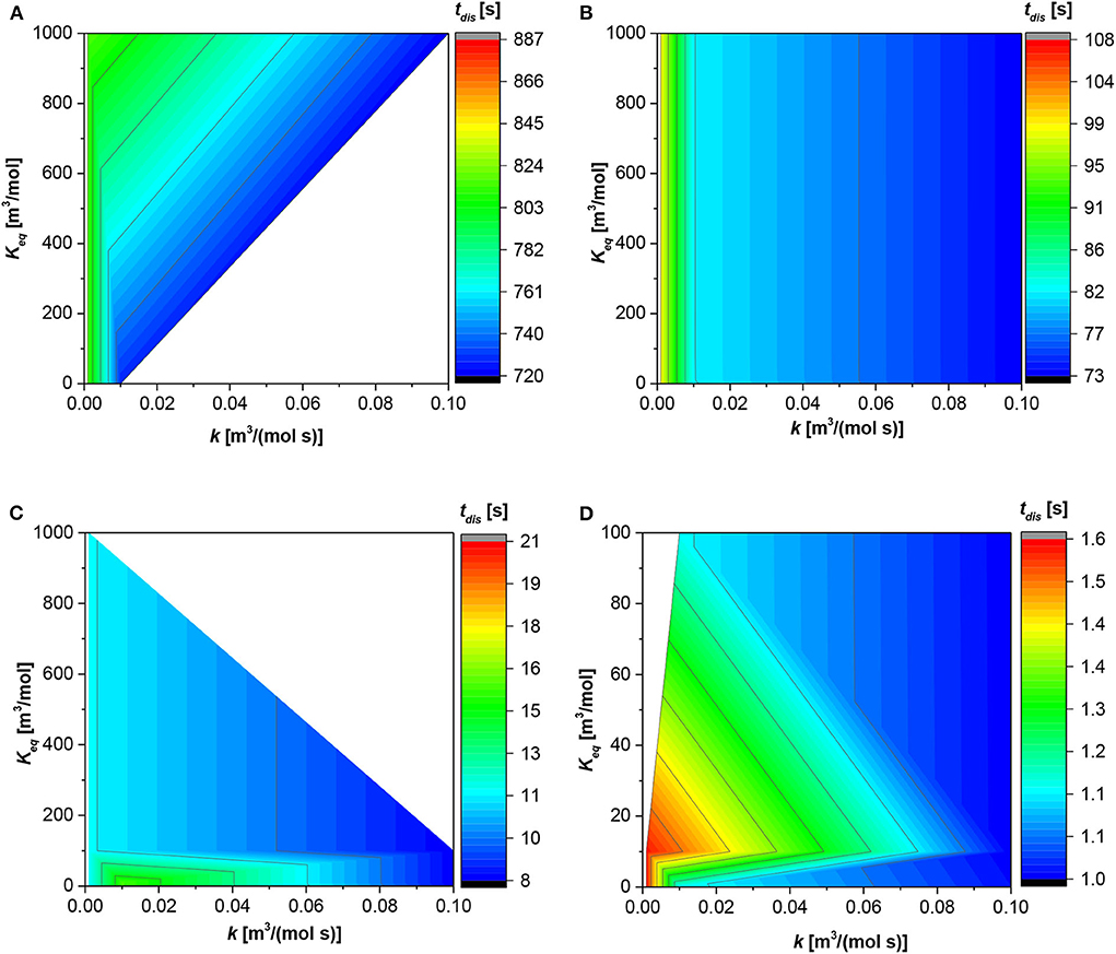
Figure 2. Contour plot for the dissolution time (tdis) along the reaction and equilibrium constant. (A) First dimensionless number (AD1) = 1 × 10⁻³ [-]; (B) AD1 = 1 × 10⁻² [-]; (C) AD1 = 1 × 10⁻¹ [-]; (D) AD1 = 1 [-].
For the lower AD1 (Figure 2A), the particle “lives” in the system for much time with respect to the other cases. The dissolution time increases by increasing the equilibrium constant, when the reaction rate constant is >0.01 [m3/(mol s)]. Contrarily, at lowest reaction rate constant (<0.01[m3/(mol s)]) the dissolution time is the same, at each equilibrium constant value.
The situation is more linear for Figure 2B in which the higher the reaction constant, the faster the dissolution time. In this case, the dissolution time is independent from the equilibrium constant; in fact, at each value of the latter, the dissolution time is the same.
About Figure 2C, the trend is in general analogous to the first two figures, the dissolution time decreases with the reaction constant; the higher the reaction constant the faster the dissolution time. The situation is different at low values of the equilibrium constant (<100 [m3/mol]); in fact, the dissolution time presents a maximum at reaction constant equal to 0.015 [m3/(mol s)], and it decreases both diminishing and increasing the reaction constant.
Finally, Figure 2D shows the situation with the higher dimensionless number (AD1 = 1), in this situation the dissolution time is lower. The trend can be divided into two ranges. The first one is for an equilibrium constant higher than 10, and the dissolution time is faster, increasing either the reaction or equilibrium constant. Contrarily, at equilibrium constant values <10 [m3/mol], the dissolution time is faster either with increasing the reaction rate constant or decreasing the equilibrium constant. The slower dissolution time for this situation is at an equilibrium constant close to 10 [m3/mol] and a lower value of the reaction rate constant.
Figure 3 shows the trend of the shift time (tshift); this time suggests when the reaction pass from the liquid film to the liquid bulk or vice versa. As demonstrates in the previous paragraph, the contribution at the bulk or film is given by the instantaneous contributions of each reaction in each phase. The trend of the shift time is quite similar to the dissolution time displayed in Figure 2. The time requested for the shift from the film to the bulk, for the first dimensionless number equal to 1 × 10⁻³, is higher than in the other three situations in which the shift time is <1 s. In this situation (Figure 3A), the higher the reaction constant the higher the shift time; however, the fixed the reaction rate constant the shift time is quite similar increasing the equilibrium constant. Regarding Figure 3B, the situation is linear. The shift time increases with the reaction constant from 0.01 [s], at the lowest value of the former for every value of equilibrium constant, to 0.15 [s] at the highest value of the former for every value of the equilibrium constant.
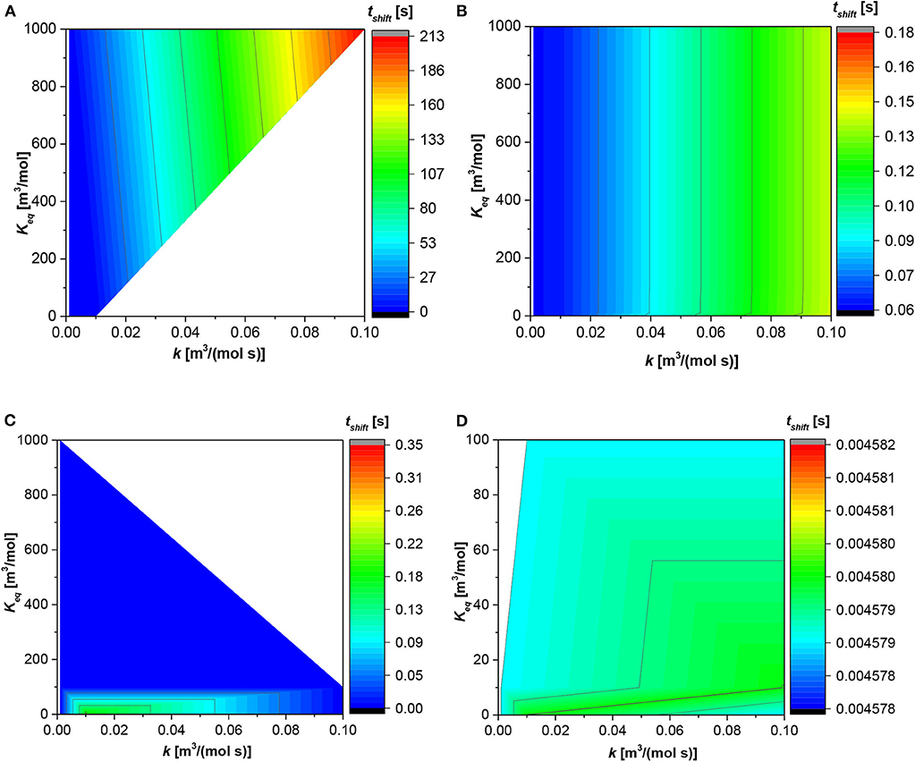
Figure 3. Contour plot for the shift time (tshift) along the reaction and equilibrium constant. (A) First dimensionless number (AD1) = 1 × 10⁻³ [-]; (B) AD1 = 1 × 10⁻² [-]; (C) AD1 = 1 × 10⁻¹ [-]; (D) AD1 = 1 [-].
Figure 3C shows an appreciable change in the shift time only for the equilibrium constant value below 100 [m3/mol]. In fact, above this magnitude, independent of the reaction constant, the shift time is the lowest. On the contrarily, under 100 [m3/mol] the maximum shift time in localized at the reaction rate constant equal to 0.02 [m3/(mol s)] and moving either at lower or higher reaction rate constant the shift time diminishes. Finally, in Figure 3D, the situation is different. The shift time presents a maximum between two local minima present at both low equilibrium and reaction constant and high reaction constant and low equilibrium constant, respectively.
Figures 4–6 represent the shift from the film to the liquid bulk with respect to some operating variable. The passage from the total contribution of the film to liquid bulk is due to the diminishing size of particle and consequently of the film thickness, as declared in the present model.
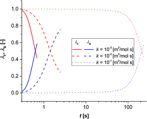
Figure 4. Contribution analysis results for bulk (blue lines) and film (red lines). Simulation conditions Di = 1 × 10⁻⁹ [m2/s], R0 = 1 × 10⁻³ [m], Keq = 0.1 [-].
In Figure 4, the time to the shift was calculated parametric with the reaction rate constant. As revealed, the shift changes of two orders of magnitude passing from 0.6 [s] when k = 1 × 10⁻³ [m3/(mol s)], to about 220 [s] when k = 1 × 10⁻¹ [m3/(mol s)].
Figure 5 shows the shift time with the diffusion of the i-component through the film as a parameter; in this case, the time for passing from the film to the bulk is instantaneous in both situations. However, a higher order of magnitude is required for the slower diffusion rate. This result is expected; in fact, a higher diffusion allows a rapid contact between the dissolved solid, and the compound in the liquid phase leads to a faster diminishing of the solid particle and film thickness. Consequently, the momentaneous contributions of the liquid bulk became higher than that of the film and the reaction pass from the latter to the former.
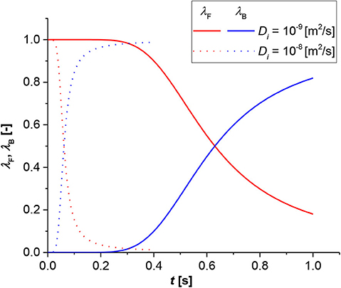
Figure 5. Contribution analysis results for bulk (blue lines) and film (red lines). Simulation conditions R0 = 1 × 10⁻³ [m], k = 1 × 10⁻³ [m3/(mol s)], Keq = 1 × 10⁻³ [-].
Figure 6 represents the shift time with the equilibrium constant as parameter. In this case, the shift time has the same order of magnitude for all the simulations within the set. The difference between the equilibrium constant equal to 1 [m3/mol] and 10 [m3/mol] is very minor. Contrarily, the shift time for the equilibrium constant value equal to 0.1 [m3/mol] is higher. This means that at higher equilibrium constants, the system approaches an irreversible state; thus, the influence of the chemical equilibrium becomes negligible on the reaction rate, and the shift time moves to lower values as the transition between film to bulk phase becomes the fastest possible.
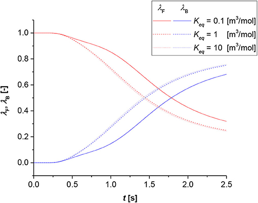
Figure 6. Contribution analysis results for bulk (blue lines) and film (red lines). Simulation conditions Di = 1 × 10⁻⁹ [m2/s], R0 = 1 × 10⁻³ [m], k = 1 × 10⁻³ [m3/(mol s)].
Finally, the model was tested on the system without reaction to evaluate the dissolution time (tdis) of the solid particle with respect to the dimensionless numbers (AD1 and AD3). In Figure 7, AD1 and AD3 were plotted vs. tdis, and not vice versa, as the figure is more illustrative as such.
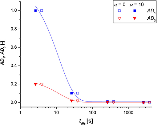
Figure 7. Dimensionless numbers (AD1 blue symbols and line, AD3 red symbols and lines) vs. the dissolution time (tdis) at α = 0 (no stirring, empty symbol) and α = 10 (high stirring value, full symbol), for a non-reactive system.
Recalling that AD1 and AD3 are both proportional to the molecular diffusivity and the reverse of the initial particle radius, the trends with the dissolution time are qualitatively similar. As revealed, by either increasing the particle radius or decreasing the molecular diffusivity, a corresponding increase of the dissolution times was calculated. This information is rather logical as bigger particles need more time to dissolve and react; the same occurs if the solute has a low molecular mobility within the stagnant liquid film. Moreover, the variations in AD1 and AD3 parameters look appreciable when increasing the dimensionless stirring parameter (α), even if the trends are logical, because by increasing the stirring rate, a lower dissolution time was estimated.
Conclusions
The ESFM was successfully applied on bimolecular solid-liquid reversible reaction kinetics. The simulations were based on a general liquid-solid reaction system in which a non-ideal shape factor of the solid was considered, revealing the flexibility and the power of the ESFM model. A detailed investigation was conducted studying the cases of reversible reaction and the analogous non-reactive system, demonstrating how the operation conditions and the physical parameters affect the performances of the system.
The reported investigation revealed that both the initial particle radius of the solid phase and the physical nature of the involved components, that is, the molecular diffusivity, are crucial factors to determine the time of shift between the regimes. Thus, grinding correctly, the solid phase could lead to faster kinetics. Moreover, the eventual presence of chemical equilibrium could reduce the overall rate of the process. The non-reactive system case confirmed the high influence of the initial particle radius and the molecular diffusivity on the dissolution time, a fact even more evident when the system is stirred at higher rates.
General hypotheses were applied to simplify the mathematical treatment; however, a more specific and appropriate model development could be considered to further improve the model, as introducing the particle size distribution, as well energy balances for highly exothermic or endothermic reactions.
Data Availability Statement
All datasets generated for this study are included in the article/supplementary material.
Author Contributions
VR: conceptualization, supervision, and formal analysis. HG: conceptualization and formal analysis. TC: software and writing—original draft. RT: software. TS: conceptualization and supervision. All authors contributed to the article and approved the submitted version.
Conflict of Interest
The authors declare that the research was conducted in the absence of any commercial or financial relationships that could be construed as a potential conflict of interest.
Acknowledgments
University of Naples Federico II is acknowledged for funding The international agreement between University of Naples Federico II (IT) and Åbo Akademi University (FI) that allowed the exchange between researchers of the two affiliations, making the realization of this work possible. The economic support from Akademi of Finland is gratefully acknowledged (Academy Professor's grant given to TS).
References
Box, J. C., and Prosser, A. P. (1989). A general model for the reaction for several minerals and several reagents in heap and dump leaching. Hydrometallurgy 16, 77–92. doi: 10.1016/0304-386X(86)90053-8
Fan, L. S., Miyanami, K., and Fan, L. T. (1977). Transient analysis of isothermal fluid-solid reactions systems: modeling the sigmoidal conversion-time behaviour of a gas-solid reaction. Chem. Eng. J. 13, 13–20. doi: 10.1016/0300-9467(77)80003-8
Gibilaro, L. J., Jioia, F., and Greco, G. (1970). Unsteady-state diffusion in a porous solid containing dead-ended pores. Chem. Eng. J. 1, 85–90. doi: 10.1016/0300-9467(70)85001-8
Green, D. W., and Perry, R. H. (2007). Perry's Chemical Engineers', 8th Edn. New York, NY: McGraw-Hill.
Jidaspow, D., Dharia, D., and Leung, L. (1976). Gas purification by porous solids with structural changes. Chem. Eng. Sci. 31, 337–344. doi: 10.1016/0009-2509(76)80002-4
Le Coenta, A. L., Tayakout-Fayollea, M., Couennea, F., Briancona, S., Lietoa, J., Fitremann-Gagnaireb, J., et al. (2003). Kinetic parameter estimation and modelling of sucrose esters synthesis without solvent. Chem. Eng. Sci. 58, 367–376. doi: 10.1016/S0009-2509(02)00474-8
Lindman, N., and Simonsson, D. (1979). On the application of the shrinking core model to liquid—solid reactions. Chem. Eng. Sci. 34, 31–35. doi: 10.1016/0009-2509(79)85175-1
Park, J. Y., and Levenspiel, O. (1975). The crackling core model for the reaction of solid particles. Chem. Eng. Sci. 30, 1207–1214. doi: 10.1016/0009-2509(75)85041-X
Ranjan Jena, P., De Jayanta, S., and Basu, K. (2003). A generalized shrinking core model applied to batch adsorption. Chem. Eng. J. 95, 143–154. doi: 10.1016/S1385-8947(03)00097-4
Russo, V., Kilpiö, T., Di Serio, M., Tesser, R., Santacesaria, E., Murzin, D. Y., et al. (2015a). Dynamic non-isothermal trickle bed reactor with both internal diffusion and heat conduction: arabinose hydrogenation as a case study. Chem. Eng. Res. Design 102, 171–185. doi: 10.1016/j.cherd.2015.06.011
Russo, V., Kilpiö, T., Hernandez Carucci, J., Di Serio, M., and Salmi, T. (2015b). Modeling of microreactors for ethylene epoxidation and total oxidation. Chem. Eng. Sci. 134, 563–571. doi: 10.1016/j.ces.2015.05.019
Russo, V., Salmi, T., Carletti, C., Murzin, D., Westerlund, T., Tesser, R., et al. (2017). Application of an extended shrinking film model to limestone dissolution. Ind. Eng. Chem. Res. 56, 13254–13261. doi: 10.1021/acs.iecr.7b01654
Salmi, T., Grénman, H., Bernas, H., Wärnå, J., and Murzin, D. Y. (2010). Mechanistic modelling of kinetics and mass transfer for a solid–liquid system: leaching of zinc with ferric iron. Chem. Eng Sci. 65, 4460–4471. doi: 10.1016/j.ces.2010.04.004
Salmi, T., Russo, V., Carletti, C., Kilpiö, T., Tesser, R., Murzin, D., et al. (2017). Application of film theory on the reactions of solid particles with liquids: shrinking particles with changing liquid films. Chem. Eng. Sci. 160, 161–170. doi: 10.1016/j.ces.2016.11.026
Temkin, M. I. (1977). Transfer of dissolved matter between a turbulently moving liquid and particles suspended in it. Kinetika i Kataliz 18, 493–496.
Verbaan, B., and Crundwell, F. K. (1986). An electrochemical model for the leaching of a sphalerite concentrate. Hydrometallurgy 16, 345–359. doi: 10.1016/0304-386X(86)90009-5
Wakao, N. (1984). Recent Analysis of Chemically Reacting Systems, eds L. K. Doraiswamy. New Delhi: Wiley Eastern.
Williams, R. J., Calvelo, A., and Cunningham, R. E. (1972). A general asymptotic analytical solution for non-catalytic gas-solid reactions. Can. J. Chem. Eng. 50, 486–490. doi: 10.1002/cjce.5450500407
Nomenclature
A surface area, m2
a surface area-to-volume ratio, m2/m3
AD1 AD1=Di τ/R02, the first dimensionless number, -
AD2 AD2 = α, the second dimensionless number, -
AD3 AD3=Dia0τ/R0, the third dimensionless number, -
AD4 AD4=c0VL/n0j, the fourth dimensionless number, -
c concentration, mol/m3
D diffusion coefficient, m2/s
k reaction rate constant, m3/(mols)
kL mass transfer coefficient, m/s
Keq equilibrium constant, m3/mol
M molar mass, kg/mol
N diffusion flux, mol/(m2·s)
n amount of substance, mol
R particle radius, m
r radial coordinate, m
s shape factor, -
T temperature, K
t time, s
V volume, m3
x dimensionless film coordinate, -
y dimensionless concentration, -
Greek letters
α dimensionless number, -
δ film thickness, m
Γ, Γ' generation rate, mol/(m3·s)
ε dissipated energy, W/kg
θ dimensionless time, -
λ normalized contribution, -
ν stoichiometric coefficient, -
υ kinematic viscosity, m2/s
τ characteristic reaction time, s
Dimensionless numbers
Re Reynolds number, -
Sc Schmidt number, -
Sh Sherwood number, -
Subscripts and superscripts
B bulk phase
F film
i liquid-phase and general component index
j solid-phase component index
L liquid phase
P particle
0 initial quantity
* saturated state
Keywords: modeling, shrinking particle, reactive solids, ESFM, film theory
Citation: Russo V, Grénman H, Cogliano T, Tesser R and Salmi T (2020) Advanced Shrinking Particle Model for Fluid-Reactive Solid Systems. Front. Chem. Eng. 2:577505. doi: 10.3389/fceng.2020.577505
Received: 29 June 2020; Accepted: 19 August 2020;
Published: 06 October 2020.
Edited by:
Vincenzo Palma, University of Salerno, ItalyReviewed by:
Heather Trajano, University of British Columbia, CanadaSimona Renda, University of Salerno, Italy
Copyright © 2020 Russo, Grénman, Cogliano, Tesser and Salmi. This is an open-access article distributed under the terms of the Creative Commons Attribution License (CC BY). The use, distribution or reproduction in other forums is permitted, provided the original author(s) and the copyright owner(s) are credited and that the original publication in this journal is cited, in accordance with accepted academic practice. No use, distribution or reproduction is permitted which does not comply with these terms.
*Correspondence: Vincenzo Russo, di5ydXNzb0B1bmluYS5pdA==