 Xian-hua Xie
 Yu-jie Huang1
 Guo-sheng Han
- 1Key Laboratory of Jiangxi Province for Numerical Simulation and Emulation Techniques, Gannan Normal University, Ganzhoiu, China
- 2Key Laboratory of Intelligent Computing and Information Processing of Ministry of Education and Hunan Key Laboratory for Computation and Simulation in Science and Engineering, Xiangtan University, Xiangtan, China
- 3School of Economics, Zhengzhou University of Aeronautics, Zhengzhou, China
Introduction: The species diversity of microbiomes is a cutting-edge concept in metagenomic research. In this study, we propose a multifractal analysis for metagenomic research.
Method and Results: Firstly, we visualized the chaotic game representation (CGR) of simulated metagenomes and real metagenomes. We find that metagenomes are visualized with self-similarity. Then we defined and calculated the multifractal dimension for the visualized plot of simulated and real metagenomes, respectively. By analyzing the Pearson correlation coefficients between the multifractal dimension and the traditional species diversity index, we obtain that the correlation coefficients between the multifractal dimension and the species richness index and Shannon diversity index reached the maximum value when q = 0, 1, and the correlation coefficient between the multifractal dimension and the Simpson diversity index reached the maximum value when q = 5. Finally, we apply our method to real metagenomes of the gut microbiota of 100 infants who are newborn and 4 and 12 months old. The results show that the multifractal dimensions of an infant's gut microbiomes can distinguish age differences.
Conclusion and Discussion: There is self-similarity among the CGRs of WGS of metagenomes, and the multifractal spectrum is an important characteristic for metagenomes. The traditional diversity indicators can be unified under the framework of multifractal analysis. These results coincided with similar results in macrobial ecology. The multifractal spectrum of infants’ gut microbiomes are related to the development of the infants.
Introduction
The study of species diversity in ecology has a long history (Kempton and Taylor, 1976; Hubalek, 2000). The diversity indices can be divided into two categories:α diversity index and β diversity index. All diversity indices referred to in this report are α diversity index which can be characterized by species richness, Shannon diversity index, and Simpson diversity index in macrobial (plants/animals). In the field of macrobial ecology, species richness increases with the increase of ecological area, and species–area relationship (SAR) can be formulated as S(A)=cA, where A is area, S(A) is the number of species in A, c and z are constants. SAR is a famous formula in ecological study (Borda-de-Água et al., 2002). On the basis of SAR, Harte and Kinzig pointed out that the formula indicates the self-similarity of species number and area (Harte and Kinzig, 1997). As a main feature of fractals, self-similarity can be described by
When q<0, zq emphasizes the character of rare species; when q>0,zq emphasizes the common species. z0 implies the relationship between the logarithm of species richness [ln(S(A))] and the logarithm of the area [ln(A)]. z1 implies the relationship between the logarithm of the Shannon diversity (SHD) index and the logarithm of the area. z2 implies the relationship between the logarithm of the Simpson diversity (SID) index and the logarithm of the area.
In microbial diversity studies, it remains a challenge to identify bacterial strains in metagenome and microbiome samples by using computational analysis of short-read sequences (Kuleshov et al., 2016); hence, the main difference in diversity indices between macrobial and microbial is that the concept of “species” has been substituted by “OTUs”. The number of operation taxonomic units (OTUs) within a community is akin to species richness within macrobial systems (Stegen et al., 2016). Similar to macrobial ecology, species richness, Shannon diversity index, and Simpson diversity index were used to describe the species diversity of a microbial community (Leinster and Cobbold, 2012). However, there is still a lack of study to unify these diversity indicators into a single framework.
Fractal analysis has been applied in DNA sequence analysis for more than 30 years (Joel, 1990; Berthelsen et al., 1992). For example, chaos game representation (CGR) is a classical method (Joseph and Sasikumar, 2006), and it can map DNA sequences into a unit square as follows:
Where PA=(0,0),Pc=(0,1),PG=(1,0), and PT=(1,1) correspond to four nucleotides A, C, G, and T, respectively, CGR0=(0.5,0.5).
According to Karamichalis et al. (2016), CGRs also have been subjected to multifractal analysis (which measures the degree of self-similarity within the image). Based on the visualization of DNA sequence, its multifractal spectrum (Vélez et al., 2010; Moreno et al., 2011) can be defined as follows:
where ϵ is the side length of grid, Mi is the count of point in the ith grid, and M0is the summation of all Mi. Furthermore, the multifractal dimensions of DNA sequence can be defined by . In practical computation, the above-mentioned formula can be rewritten as follows:
Then, D(q) can be calculated by linear fitting and ln(ϵ) (Vélez et al., 2010; Moreno et al., 2011).
Inspired by Karamichalis et al. (2016), the research group of Vélez studied the Caenorhabditis elegans genome (Vélez et al., 2010) and the human genome (Moreno et al., 2011) by multifractal formalism. Their results showed that the human (Homo sapiens) genome has stronger multifractality than that of C. elegans at the chromosome level. Similarly, Zhou et al. (2005) studied the discrimination problem of coding and non-coding DNA sequence. Their results suggest that coding and non-coding DNA sequence have different multifractal characteristics in the same genome. Pandit et al. (2012) studied the classification of HIV-1 by using multifractal dimensions of genomes. These results suggested that multifractal characteristics can measure the complexity of genes and genomes. Recently, Olyaee et al. used the CGR method to extract several valuable features from genomic sequences of SARS-CoV-2 (Olyaee et al., 2020). In 2021, Kania and Sarapata, 2021 studied the robustness of the chaos game representation to mutations and its application in an alignment-free method. On the basis of fractal scaling analysis, latterly, Meraz et al. (2022) characterized the organization of the SARS-CoV-2 genome sequence.
In order to further study the generalization of CGR, in 2019, Ge et al., 2019 generalized CGR to higher-dimensional spaces while maintaining its bijection, keeping such a method sufficiently representative and mathematically rigorous compared to previous attempts. In this frame, Dick and Green studied the proteome-wide protein prediction problem by chaos game representations and deep learning (Dick and Green, 2020). Ni et al. (2021) studied the gene sequence phylogenetic problem by frequency chaos game representation with perceptual image hashing.
For additive methods for genomic signatures of CGR, Karamichalis et al. (2016) reported their research results. They proposed the general concept of additive DNA signature of a set (collection) of DNA sequences. For example, the composite DNA signature combines information from DNA fragments and organellar, and the assembled DNA signature combines information from many short DNA subfragments (e.g., 100 base pairs) of a given DNA fragment. They concluded that such additive signatures could be used with raw unassembled next-generation sequencing (NGS) read data when high-quality sequencing data are not available.
Motivated by Karamichalis et al. (2016), in this study, we apply the fractal and multifractal methods to species diversity analysis of microbiomes. First, we visualize the simulated metagenomes and real metagenomes. Then, we compute the multifractal dimensions of simulated metagenomes and study the relationship between their multifractal dimensions and species diversity indices. Last, we compute multifractal dimensions of real metagenomes of 100 infants’ gut microbiomes when they are newborn, 4 months, and 12 months.
Materials, methods, and results
Metagenome datasets
The whole genomic sequences (WGS) (.fasta files) were downloaded from the NCBI database (ftp://ftp.ncbi.nlm.nih.gov/genomes/). The WGS for real metagenomes (.gz files) were downloaded from the NCBI SRA database (https://www.ncbi.nlm.nih.gov/sra).
Dataset 1: Simulated high-diversity metagenome set generated from the genomes of 10 distantly related major bacterial species used in Dubinkina et al. (2016). For each simulated metagenome, the number of reads is 10M and the read length is 1,000 bp. The high-diversity set includes 100 metagenomes generated from the genomes of 10 distantly related major bacterial species accounting for more than 90% of all reads in the Chinese group. The species used in dataset 1 are listed in Table 1. The abundances in dataset 1 are listed in Supplementary Table S1. In this simulation, the number of reads is 100 K and the read length is 1,000 bp.
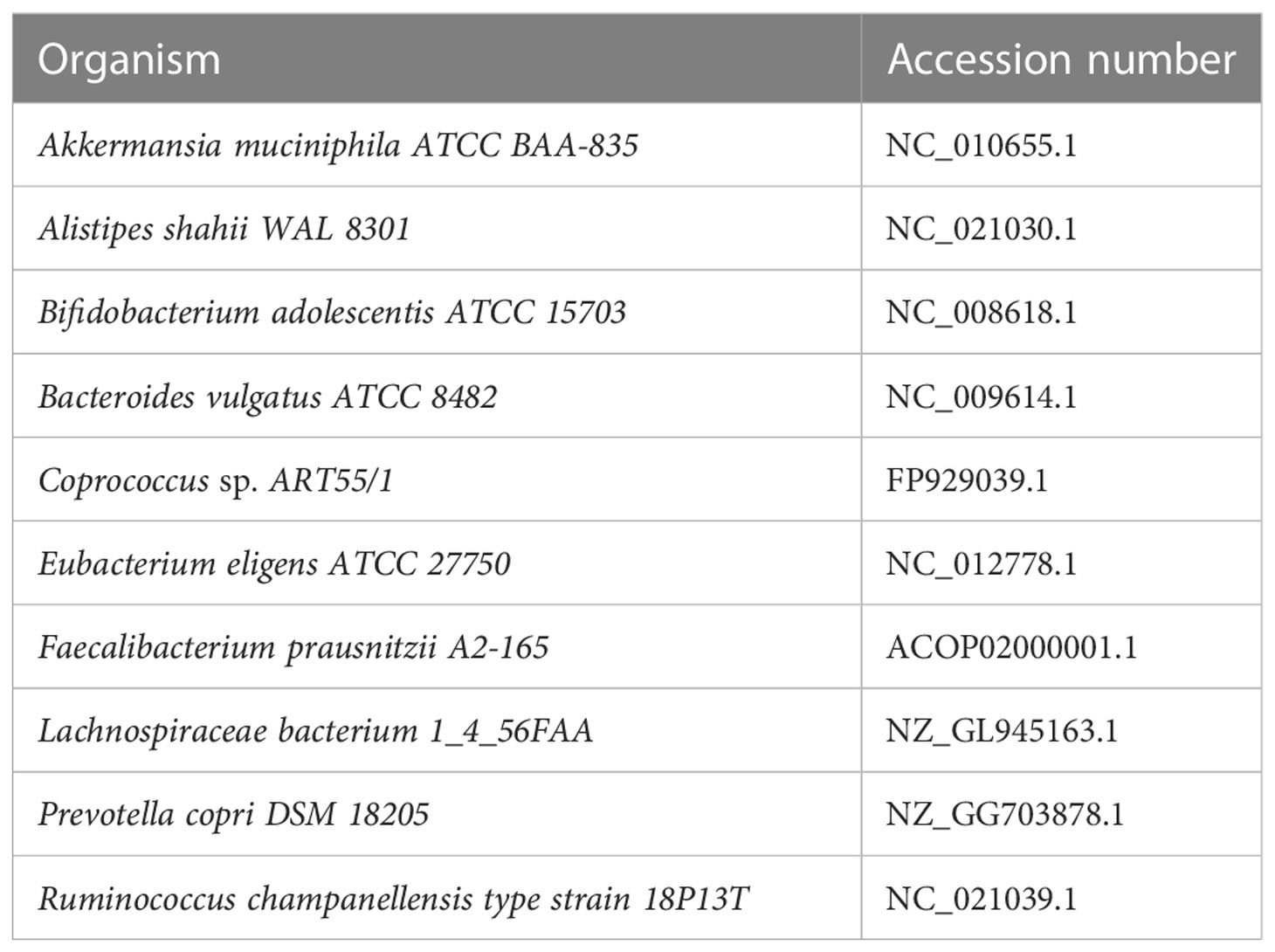
Table 1 Species and accession numbers used in dataset 1.
Dataset 2: Simulated low-diversity metagenome set generated from the genomes of 10 closely related major bacterial species used in Dubinkina et al. (2016). The species used in dataset 2 are listed in Table 2. The abundances in dataset 2 are listed in Supplementary Table S2. In this simulation, the number of reads is 100 K and the read length is 1000 bp.
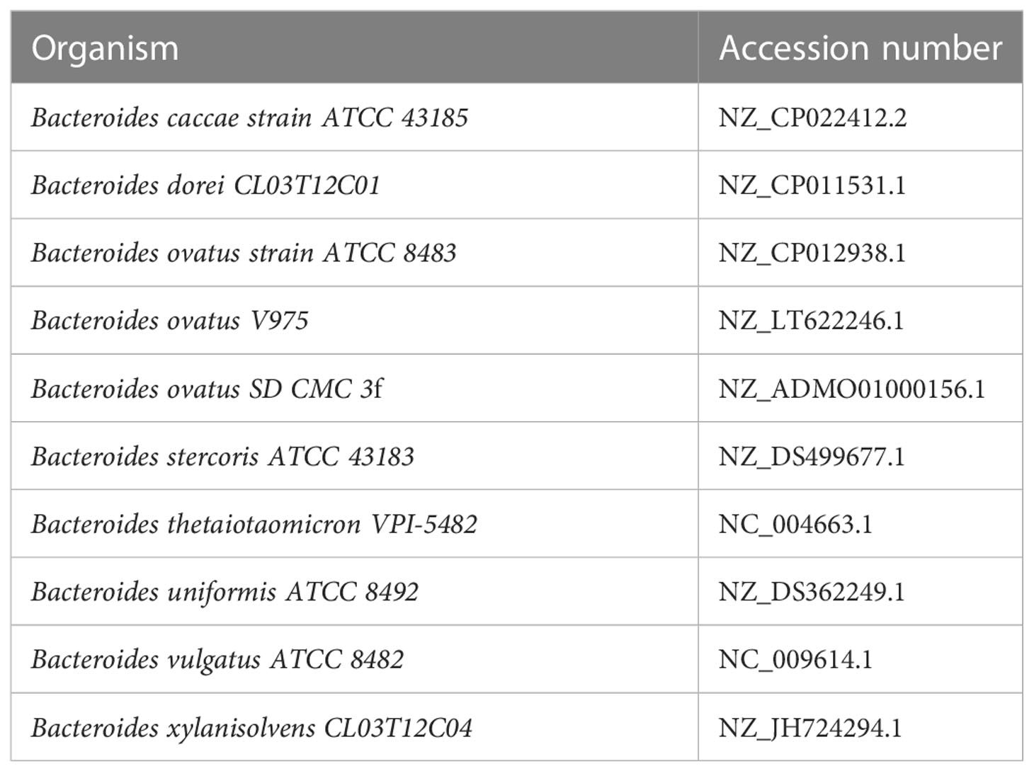
Table 2 Species and accession numbers used in dataset 2.
Dataset 3: There are 400 WGS for real metagenomes of 100 infants’ and their mother’s gut microbiota. It includes 300 infants’ fecal metagenomes when they are newborn, 4 months, and 12 months, and 100 fecal metagenomes of their mothers. This dataset was used in Bäckhed et al. (2015) and the accession number is PRJEB6456. The study was approved by the Regional Ethical Review Board in Lund. Informed consent was obtained from all mothers.
Visualization of metagenomes
Consider the alphabet Ω={A, C, G, T} and let S={s1,s2, ,sm} be a WGS metagenome dataset, we set si=si1si2 si,ni as the ith reads in S, and sik∈Ω is the kth nucleotide of reads si. To represent a WGS dataset of metagenome in the form of a CGR plot, a unit square was used, whose four vertices were labeled as A=(0,0), C=(0,1), G=(1,0), and T=(1,1). For a given metagenome dataset S={ s1,s2,⋯,sm } , which includes m reads, the kth nucleotide of reads corresponds to CGRik=CGRi,k-1+0.5*(Pik-CGRi,k-1,Pi=PA,PC,PG, or PT, i=1,2,…,m, where PA=(0,0), PC=(0,1), PG=(1,0), and PT=(1,1) correspond to the four nucleotides A, C, G, and T, respectively,CGRi0=(0.5,0.5). In order to avoid “large number annihilating small number”, we discarded the first 10 points of each read.
Based on the plotting point above, we split the unit square into 256 × 256, 512 × 512, 1,024 × 1,024, and 2,048 × 2,048 small squares in turn and then we counted the number of points in every small square. Figure 1 is an example of dataset 2.
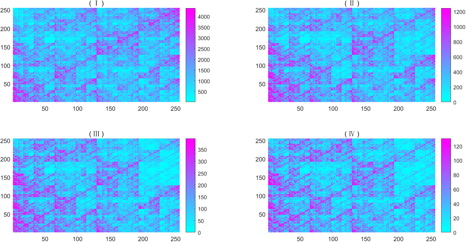
Figure 1 Heat map of simulated metagenome of dataset 2, the abundance are 0.016928832, 0.30559462, 0.120814049, 0, 0.07959993, 0.00894306, 0.03682631, 0.37768779, 0.00570905, and 0.04789635. The dissolution of (I) is 256×256; (II) is an image magnified by a factor of 2 from the upper left part of (I); (III) is an image magnified by a factor of 2 from the upper left part of (II); and (IV) is an image magnified by a factor of 2 from the upper left part of (III). For better visibility, we regarded the number exceeding the threshold as the threshold, whose values are taken three times the mean value.
Fractal and multifractal spectrum of metagenome
From Figure 1, we found that all CGRs seem to be self-similar. Thus, we intended to study their fractal and multifractal properties. On the basis of visualization of metagenome sequence, one can define its multifractal spectrum by Eq. (1).
Furthermore, one can define multifractal dimension by . In practical computation, one can compute D(q) by linear fitting between ln(M(ϵ,q)) and ln(ϵ) according to Eq. (2). Figure 2 shows the linear fit between (i.e., ln(M(ϵ,q))) and ln(ϵ) of the simulated metagenome.
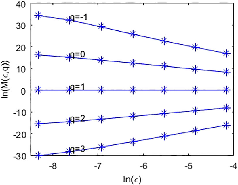
Figure 2 Linear fit of ln(M(ϵ,q)) and ln(ϵ), where ϵ is set to 2-6,2-7,2-8,2-10,2-11,2-12, and 2-13, respectively.
In metagenomic research, for a given community, a WGS dataset of metagenome is actually a collection of simple random-sampling reads from the given community (i.e., the abundance values of bacteria is fixed). In this experiment, we simulated 100 metagenomes from a given abundance of 10 bacteria. Figure 3 demonstrates the multifractal dimensions of 100 simulated metagenomes (i.e., 100 simple random samplings) from dataset 1 and 100 simulated metagenomes from dataset 2. In a modest PC [Intel(R) Core(TM) i7-9750H CPU @ 2.60GHz, 8 GB RAM], the present method only needs 6 h 54 m 43 s for computing the multifractal dimensions of 100 simulated metagenomes from dataset 1 and 6 h 50 m 42 s for computing the multifractal dimensions of 100 simulated metagenomes from dataset2.
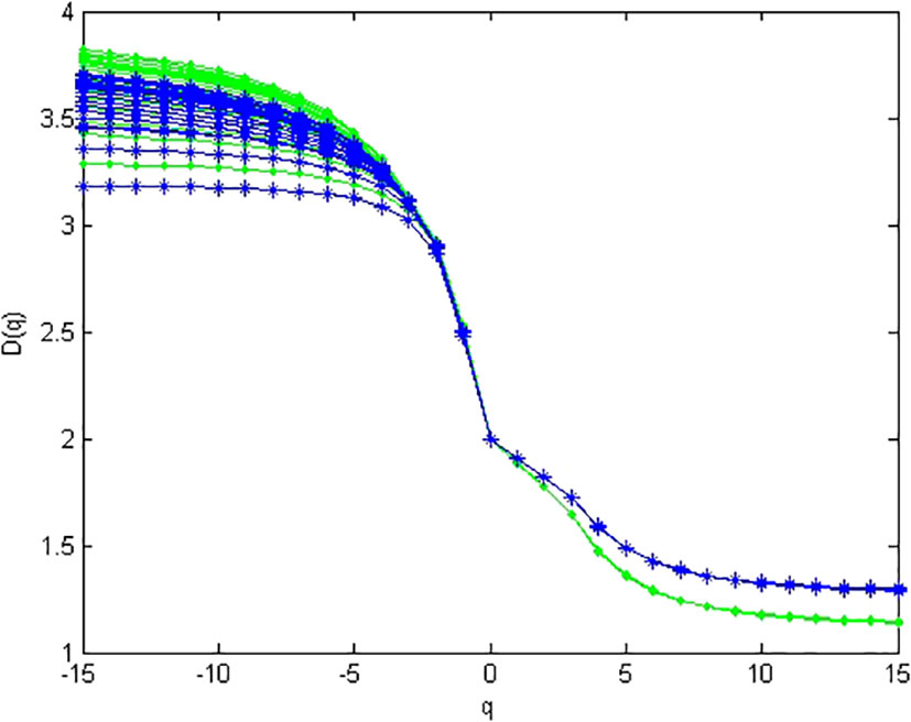
Figure 3 Multifractal dimensions of simulated genome. Green asterisks represented the D(q) of samples simulated from high-diversity communities, and blue dots represented the D(q) of samples simulated from low-diversity communities. For each sample from the same community, the abundances are given in Table S1 (the last line in the table).
From Figure 3, we can find that multifractal dimension curves of different simulated metagenomes from the same abundance are unstable when q < 0, and they are stable when q ≥ 0. Hence, we only consider D(q) for q ≥ 0 in the multifractal spectrum of metagenome.
The relationship between multifractal spectrum and microbial diversity indices of metagenomes
In order to study the relationship between the multifractal spectrum and diversity indices of metagenomes, we simulated 100 metagenomes whose abundance is known, and then their species richness index, Shannon diversity index, Simpson diversity index, and multifractal dimensions are calculated. Based on these results, the Pearson correlation coefficients are calculated according to varying q.
The Pearson correlation coefficients between species richness diversity indices and multifractal dimension are plotted in Figure 4. The plot suggests that the Pearson correlation coefficient between species richness indices and multifractal dimensions reach its maximum (0.85) at q = 0. Similarly, the Pearson correlation coefficients (Figure 5) between species Shannon diversity indices and multifractal dimensions reach its maximum (0.88) at q = 1. The Pearson correlation coefficient (Figure 6) between species Simpson diversity indices and multifractal dimensions reaches 0.87 at q = 2, while the Pearson correlation coefficients between species Simpson diversity indices and multifractal dimensions reach their maximum (0.89) at q = 5.
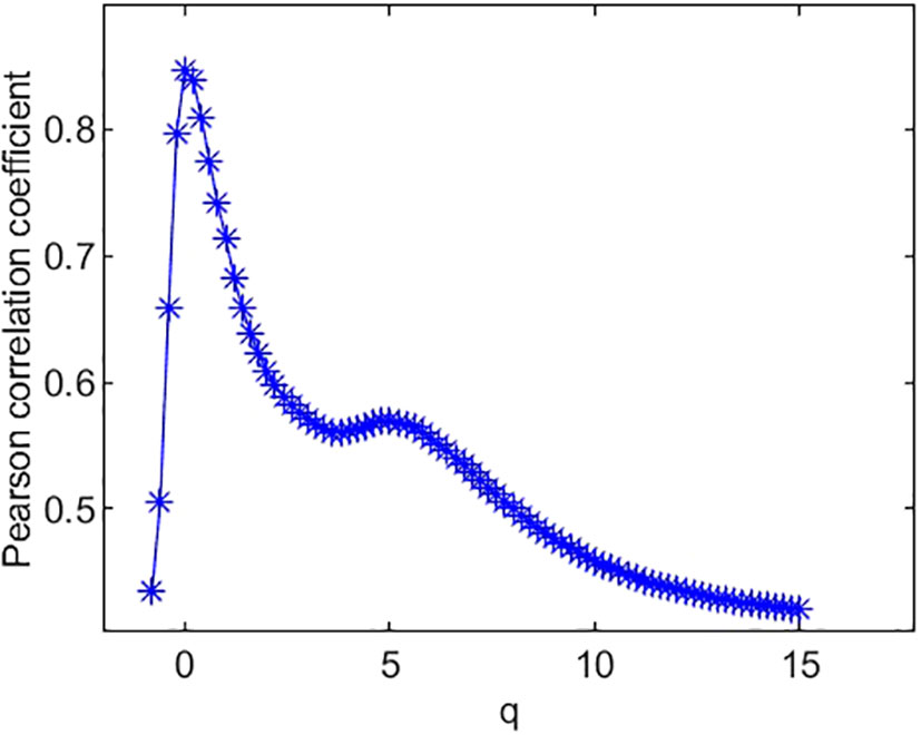
Figure 4 Pearson correlation coefficient of species richness and multifractal dimension D(q).
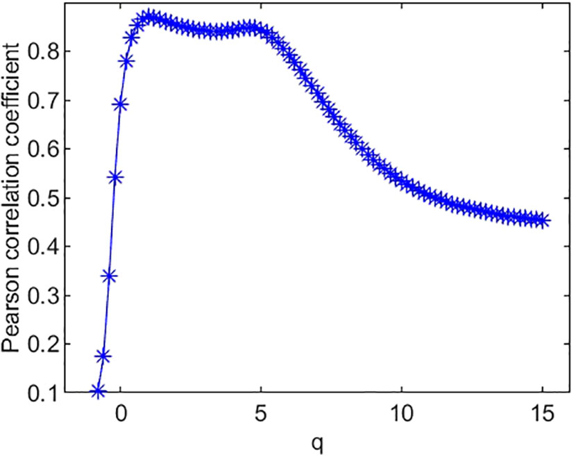
Figure 5 Pearson correlation coefficient of species’ Shannon diversity index and multifractal dimension D(q).
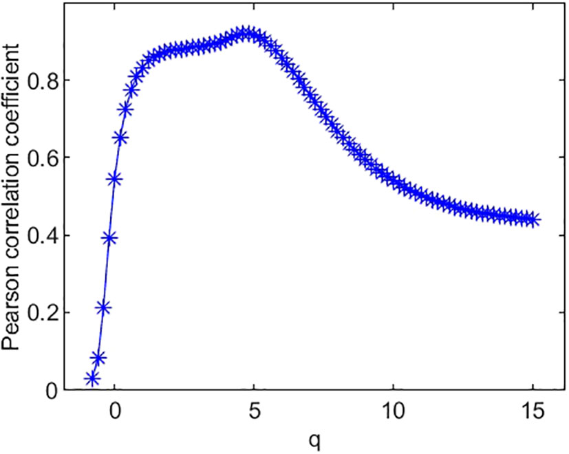
Figure 6 Pearson correlation coefficient of species’ Simpson diversity index and multifractal dimension D(q).
Application of multifractal dimension in metagenomes to infant’s gut microbiome
In order to apply the multifractal analysis to real metagenomes, we selected 100 infants’ fecal WGS datasets of 300 metagenomes [there are three samples, including 12 months (12 M), 4 months (4 M), and newborn (baby) for each infant] and 100 corresponding gut metagenomes of their mothers to mine potential information of its multifractal dimensions.
As an example, we plotted multifractal dimensions of a selected gut microbiome of a baby in Figure 7. The plot demonstrates the multifractal dimensions of gut microbiomes of an infant and his/her mother when he/she is a newborn (baby) and 4 months and 12 months old. Our method consumed 23 h 5 m 46 s for multi-fractal dimensions of the 400 metagenomes. Figure 9 suggests that the D(0) (fractal dimension),D(1) (information dimension), and D(2) (correlation dimension) are increasing with growth. In other words, their gut microbial diversity is developing with growth. In order to study the generality of this property, we calculated the mean value and standard deviation of 100 multifractal dimensions of infants at 12 months and 4 months, when they were a baby, and their mothers, respectively.
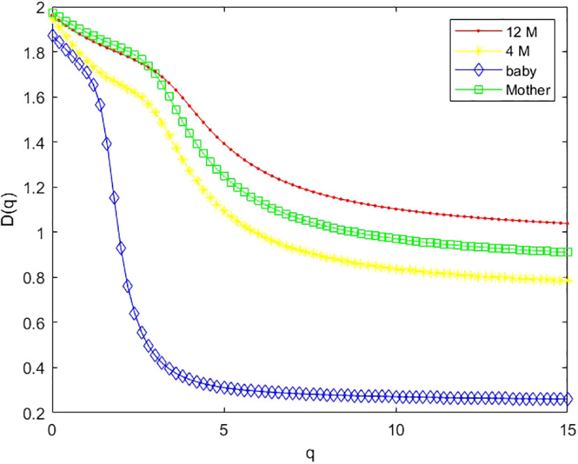
Figure 7 Multifractal dimension of the gut microbiome of the infant when he/she is 12 months old (12 M), 4 months old (4 M), and a newborn baby (baby), and her mother (M).
From Figure 8, we also found that D(0), D(1), and D(2) are increasing with growth in total. In order to obtain the statistical significance of these results, we tested their statistical significance, the results of which are shown in Table 3. From Table 3, we conclude that D(0), D(1), and D(2) are increasing with the growth in statistical significance.
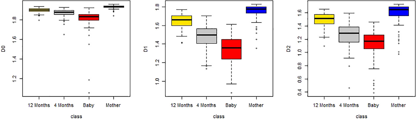
Figure 8 Boxplots of D(0), D(1), and D(2) of multifractal dimension of gut microbiomes of infants when they are 12 months old, 4 months old, and a baby, and that of the mother.
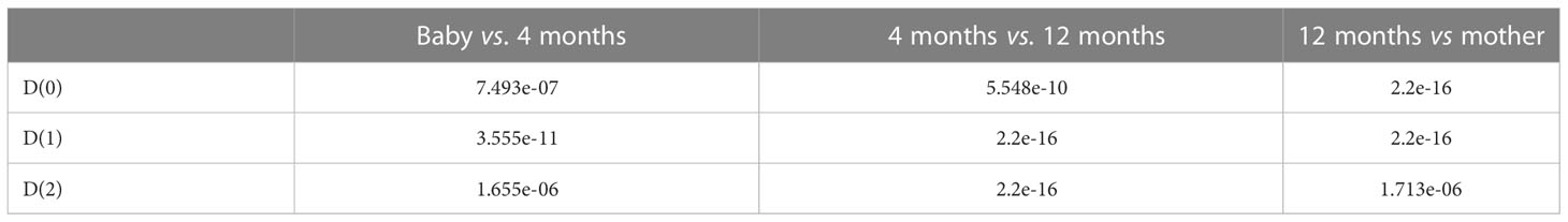
Table 3 p-values of the one-sided t-test of dataset 3 (alternative hypothesis: less).
For dataset 3, there are 100 infants’ gut microbiomes. We grouped each infant gut micobiome as one group, and there are 100 groups of gut microbiomes. For each group, we calculated the difference between 12 months and 4 months, 12 months and newborn, and 4 months and newborn, respectively. In order to observe the overall characteristics of these multifractal dimensions, we plotted the mean value of 100 multifractal dimensions of gut microbiomes in Figure 9. From Figure 9, we can draw similar conclusions to the above.
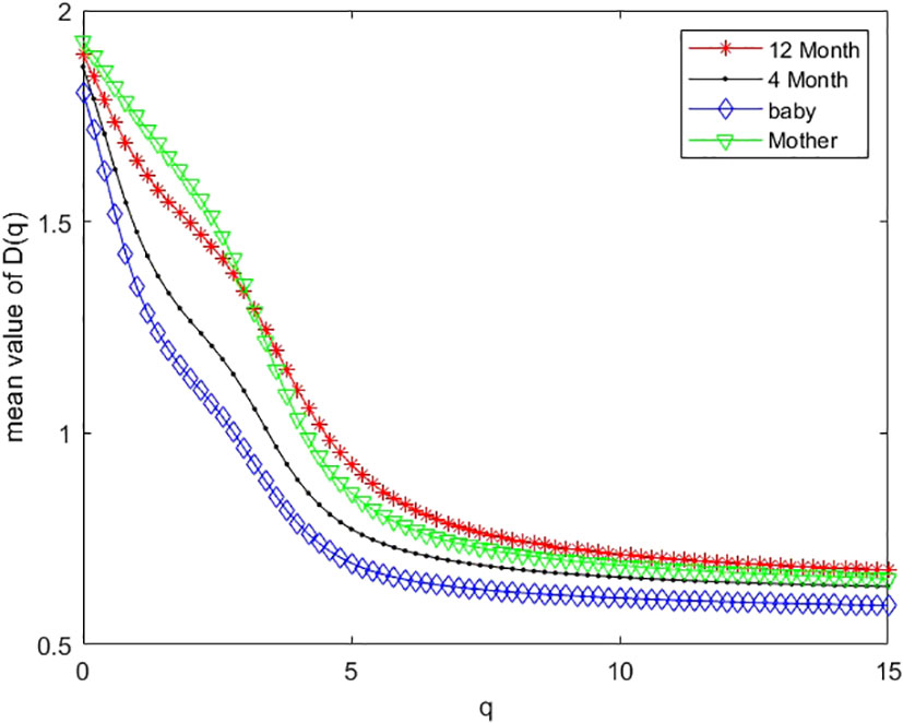
Figure 9 Mean values of multifractal dimension of 100 infants’ gut microbiomes when they are 12 months old (12 M), 4 months old (4 M), and a newborn baby (baby), and that of their mother (M).
In order to evaluate the discriminating power of gut microbiomes’ multifractal dimensions in ages of infants, we used multifractal dimensions D(q) (q from to 15 with step 0.2) of infants at 12 months and 4 months, when they were a baby, and the mothers’ gut microbiomes to discriminate by linear discriminant analysis (LDA) in R (Xu et al., 2021). It consumed only 87 s to differentiate. Table 4 demonstrates the back discriminant results of infants at 12 months and 4 months, when they were a baby, and mothers by LDA. From Table 4, we know that the accurate rate of the mothers’ gut microbiomes (90 out of 100) is best discriminated by multifractal dimensions. We also apply LDA with leave-one-out cross-validation to the dataset; the accuracy rate is 74.79%.
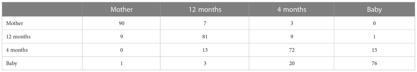
Table 4 Table of back discriminating results of 400 metagenomes.
Discussion and conclusions
In this study, we studied metagenomes by multifractal analysis. From the results above, we obtained the following conclusions:
(i) From the CGR visualization of metagenomes (Figure 1), we find that there exists statistical self-similarity in these CGR visualizations of metagenomes. From Figure 2, we concluded that there is linearity between (i.e., ln(M(ϵ,q))) and ln(ϵ) for simulated WGS metagenomes. Figure 3 demonstrates 100 simulated WGS metagenome samples from two given abundance, suggesting that the D(q) of metagenomes is stable when q≥0 and unstable when q<0 [as we know, when q<0, D(q) emphasizes the rare species (k-mers); in nature, reads of metagenome were sampled from microbial genomes, and the copy numbers of rare k-mers are unstable, so that D(q) was unstable]. These results guide us to study multifractal dimensions of metagenomes only for q≥0 in the following study. These results show that there is a multifractal character in CGRs of WGS of metagenomes.
(ii) From Figure 4, we can see that the Pearson correlation coefficients of species richness indices and D(q) reach their maximums when q=0. Similarly, we can find that the Pearson correlation coefficients of Shannon diversity indices and D(q) reach their maximums when q=1 from Figure 5, and that the Pearson correlation coefficients of Simpson diversity indices and D(q) approach their maximums when q=2 (the maximums are valued at q=5) from Figure 6. These results roughly coincide with the results of macrobial ecology in [4]. On the whole, the scatter plot of Shannon diversity indices and the corresponding D(1) demonstrated in Figure 5 show that D(1) is increasing with the increase of Shannon diversity indices of metagenomes. Figure 6 shows that D(2) is increasing with the increase of Simpson diversity indices of metagenomes. These results show that there are linearly correlated relationships between multifractal dimensions and traditional diversity indices. They also suggest that multifractal dimensions can reflect the microbial diversity in metagenomic research and the traditional diversities can be unified by the frame of multifractal analysis.
(iii) In research on real metagenomes, the multifractal dimensions of the gut microbiome of one mother and her baby are demonstrated in Figure 7; this plot shows that the multifractal dimensions of gut microbiome of baby are increasing with the infants (newborn, 4 months, and 12 months). The boxplot of Figures 8, 9 show that this law holds on the whole for babies on average. The back discriminant results of multifractal dimensions of gut microbiomes of infants demonstrated in Table 3 show that the infants’ age can be discriminated by their multifractal spectrum of CGR visualization of gut microbiomes in total. Specifically, newborn results are the best. The gut microbiomes of a 4-month-old baby can be confused more easily. For leave-one-out cross-validation, the accurate rate reached 74.97%, suggesting that the multifractal spectrum of gut microbiomes for infants can discriminate their ages powerfully.
In conclusion, there is self-similarity among the CGRs of WGS of metagenomes, and the multifractal spectrum is an important characteristic for metagenomes. The multifractal spectrum of metagenomes is related to species diversity and the development of gut microbiomes of infants.
In our study, the advantages were that the algorithm does not need alignment and that it required less computing resources than aligned methods. The disadvantage was that the algorithm cannot obtain a detailed composition and species abundance from metagenomes.
Data availability statement
The datasets presented in this study can be found in online repositories. The names of the repository/repositories and accession number(s) can be found in the article/Supplementary Material.
Ethics statement
The studies involving human participants were reviewed and approved by the Regional Ethical Review. Written informed consent to participate in this study was provided by the participants’ legal guardian/next of kin.
Author contributions
Conceptualization, X-HX and Y-LM. Methodology, X-HX and Z-GY. Software, X-HX and Y-LM. Validation, X-HX, Y-LM, Z-GY and G-SH. Formal analysis, X-HX and Y-JH. Resources, X-HX. Data curation, X-HX. Writing—original draft preparation, X-HX and Z-GY. Writing—review and editing, X-HX and Z-GY. Visualization, X-HX. Supervision, Z-GY. All authors contributed to the article and approved the submitted version.
Funding
This research was funded by the National Natural Science Foundation of China (11871061), the Natural Science Foundation of Jiangxi province (2021BAB201006), the open project of Key Laboratory of Intelligent Computing and Information Processing of Ministry of Education (Xiangtan University) grant number 2018ICIP04, and the Science and Technology Project of Jiangxi Provincial Education Department, grant number GJJ170820.
Conflict of interest
The authors declare that the research was conducted in the absence of any commercial or financial relationships that could be construed as a potential conflict of interest.
Publisher’s note
All claims expressed in this article are solely those of the authors and do not necessarily represent those of their affiliated organizations, or those of the publisher, the editors and the reviewers. Any product that may be evaluated in this article, or claim that may be made by its manufacturer, is not guaranteed or endorsed by the publisher.
Supplementary material
The Supplementary Material for this article can be found online at: https://www.frontiersin.org/articles/10.3389/fcimb.2023.1117421/full#supplementary-material
Supplementary Table 1 | The abundances in dataset 1
Supplementary Table 2 | The abundances in dataset 2.
References
Bäckhed, F., Roswall J. Peng, Y., Feng, Q., Jia Petia, H. K., et al (2015). Dynamics and stabilization of the human gut microbiome during the first year of life. Cell Host Microbe 17, 690–703. doi: 10.1016/j.chom.2015.04.004
Berthelsen, C. L., Glazier, J. A., Skolnick, M. H. (1992). Global fractal dimension of human DNA sequences treated as pseudorandom walks. Phys. Rev. A 45, 8902. doi: 10.1103/PhysRevA.45.8902
Borda-de-Água, L., Hubbell, S. P., McAllister, M. (2002). Species-area curves, diversity indices, and species abundance distributions: A multifractal analysis. Am. Nat. 159, 138–155. doi: 10.1086/324787
Dick, K., Green, J. R. (2020). “Chaos game representations & deep learning for proteome-wide protein prediction,” in 2020 IEEE 20th international conference on bioinformatics and bioengineering (BIBE) (IEEE).
Dubinkina, V., Ischenko, D., Ulyantsev, V., Tyakht, A., Alexeev, D. (2016). Assessment of k-mer spectrum applicability for metagenomic dissimilarity analysis. BMC Bioinf. 17, 38. doi: 10.1186/s12859-015-0875-7
Ge L. Liu, J., Zhang, Y., Dehmer, M. (2019). Identifying anticancer peptides by using a generalized chaos game representation. J. Math. Biol. 78, 441–463. doi: 10.1007/s00285-018-1279-x
Harte, J., Kinzig, A. P. (1997). On the implications of species-area relationships for endemism, spatial turnover, and food web patterns. Oikos 80, 417. doi: 10.2307/3546614
Hubalek, Z. (2000). Measures of species diversity in ecology: an evaluation. Folia ZOOL 49, 241–260. doi: 10.1159/000021733
Joel, J. H. (1990). Chaos game representation of gene structure. Nucleic Acids Res. 8, 2163–2170. doi: 10.1093/nar/18.8.2163
Joseph, J., Sasikumar, R. (2006). Chaos game representation for comparison of whole genomes. BMC Bioinf. 7, 243. doi: 10.1186/1471-2105-7-243
Kania, A., Sarapata, K. (2021). The robustness of the chaos game representation to mutations and its application in free-alignment methods. Genomics 113 (3), 1428–1437. doi: 10.1016/j.ygeno.2021.03.015
Karamichalis, R., Kari, L., Konstantinidis, S., Kopecki, S., Reyes, S. (2016). Molecular distance maps: An alignment-free computational tool for analyzing and visualizing DNA sequences,Doctor of philosophy (Ontario, Canada: The University of Western Ontario).
Kari, L., Konstantinidis, S., Kopecki, S., Reyes, S. (2016). Additive methods for genomic signatures. BMC Bioinf. 17, 313. doi: 10.1186/s12859-016-1157-8
Kempton, R. A., Taylor, L. R. (1976). Models and statistics for species diversity. Nature 262, 818–820. doi: 10.1038/262818a0
Kuleshov, V., Jiang, C., Zhou, W., Jahanbani, F., Batzoglou, S., Snyder, M., et al. (2016). Synthetic long-read sequencing reveals intraspecies diversity in the human microbiome. Nat. Biotechnol. 34, 64–69. doi: 10.1038/nbt.3416
Leinster, T., Cobbold, C. A. (2012). Measuring diversity: the importance of species similarity. Ecology 93, 477–489. doi: 10.1890/10-2402.1
Meraz, M., Vernon-Carter, E. J., Rodriguez, E., Alvarez-Ramirez, J. (2022). A fractal scaling analysis of the SARS-CoV-2 genome sequence. Biomed. Signal Process. Control 73, 103433. doi: 10.1016/j.bspc.2021.103433
Moreno, P. A., Patricia, E., Vélez, E., Garreta, L. E., Díaz, N., Amador, S., et al. (2011). The human genome: A multifractal analysis. BMC Genomics 12, 506. doi: 10.1186/1471-2164-12-506
Ni, H., Mu, H., Qi, D. (2021). Applying frequency chaos game representation with perceptual image hashing to gene sequence phylogenetic analyses. J. Mol. Graphics Model. 107, 107942. doi: 10.1016/j.jmgm.2021.107942
Olyaee, M. H., Pirgazi, J., Khalifeh, K., Khanteymoori, A. (2020). RCOVID19: Recurrence-based SARS-CoV-2 features using chaos game representation. Data Brief 32, 106144. doi: 10.1016/j.dib.2020.106144
Pandit, A., Dasanna, A. K., Sinha, S. (2012). Multifractal analysis of HIV-1 genomes. Mol. Phylogenet. Evol. 62, 756–763. doi: 10.1016/j.ympev.2011.11.017
Stegen, J. C., Hurlbert, A. H., Bond-Lamberty, B., Chen, X., Anderson, C. G., Chu, R. K., et al. (2016). Aligning the measurement of microbial diversity with macroecological theory. Front. Microbiol. 7, 1487. doi: 10.3389/fmicb.2016.01487
Vélez, P. E., Garreta, L. E., Martínez, E., Diaz, N., Amador, S., Tischer, I., et al. (2010). The caenorhabditis elegans genome: a multifractal analysis. Genet. Mol. Res. Gmr 9, 949. doi: 10.4238/vol9-2gmr756
Xu, L., Raitoharju, J., Iosifidis, A., Gabbouj, M. (2021). Saliency-based multilabel linear discriminant analysis. IEEE Trans. Cybernetics PP (99), 1–14. doi: 10.1109/TCYB.2021.3069338
Keywords: diversity index, multifractal, metagenome, gut metagenome, chaos game representation (CGR)
Citation: Xie X-h, Huang Y-j, Han G-s, Yu Z-g and Ma Y-l (2023) Microbial characterization based on multifractal analysis of metagenomes. Front. Cell. Infect. Microbiol. 13:1117421. doi: 10.3389/fcimb.2023.1117421
Received: 06 December 2022; Accepted: 09 January 2023;
Published: 26 January 2023.
Edited by:
Qi Wu, Institute of Microbiology (CAS), ChinaReviewed by:
Jingbo Xia, Huazhong Agricultural University, ChinaLifeng Zhu, Nanjing Normal University, China
Xu Shaoyuan, Hanshan Normal University, China
Copyright © 2023 Xie, Huang, Han, Yu and Ma. This is an open-access article distributed under the terms of the Creative Commons Attribution License (CC BY). The use, distribution or reproduction in other forums is permitted, provided the original author(s) and the copyright owner(s) are credited and that the original publication in this journal is cited, in accordance with accepted academic practice. No use, distribution or reproduction is permitted which does not comply with these terms.
*Correspondence: Xian-hua Xie, eHhpYW5odWFAc2luYS5jb20uY24=