Application of a novel numerical simulation to biochemical reaction systems

Recent advancements in omics and single-cell analysis highlight the necessity of numerical methods for managing the complexity of biological data. This paper introduces a simulation program for biochemical reaction systems based on the natural number simulation (NNS) method. This novel approach ensures the equitable treatment of all molecular entities, such as DNA, proteins, H₂O, and hydrogen ions (H⁺), in biological systems. Central to NNS is its use of stoichiometric formulas, simplifying the modeling process and facilitating efficient and accurate simulations of diverse biochemical reactions. The advantage of this method is its ability to manage all molecules uniformly, ensuring a balanced representation in simulations. Detailed in Python, NNS is adept at simulating various reactions, ranging from water ionization to Michaelis–Menten kinetics and complex gene-based systems, making it an effective tool for scientific and engineering research.

1 Introduction

In recent years, single-cell and multi-omics data analysis has attracted attention in the field of molecular cell biology (Lim et al., 2023; Massimino et al., 2023; Baysoy et al., 2024). In particular, analysis using machine learning models, such as deep learning, has been active (Lin et al., 2022; Gunawan, et al., 2023; Wagle et al., 2024). However, understanding stoichiometric reactions is still considered essential to understand gene expression and protein enzyme functions in detail. This paper proposes a simulation program for biochemical reaction systems based on the natural number simulation (NNS) method. NNS offers a simplified approach for modeling biochemical reactions stoichiometrically and performing computations of the time course of the reactions. This method excels in its straightforward formulation process and is particularly suitable for complex biological systems (Blinov et al., 2004; Browning et al., 2022; Huizing et al., 2022) because of the absence of complicated reaction formulas using mathematical equations.

Various models have been considered to represent complex biological systems, including ordinary differential equations and Gillespie’s algorithm (Gillespie, 1977; Ullah and Wolkenhauer, 2011; Alon, 2019). For example, metabolic reaction systems continue to be vigorously analyzed in detail using differential equations (Khodayari and Maranas, 2016; Himeoka and Mitarai, 2022). Petri nets substantially contribute to analyzing biochemical reaction networks by integrating stochastic algorithms and/or non-parametric strategies. This progression has resulted in the emergence of specialized forms such as signaling Petri nets, large-scale metabolic models, and multilevel biological models using colored Petri nets, indicating their increasing utility in the analysis of complex systems (Ruths et al., 2008; Rohr, 2018; Brinkrolf et al., 2021; Shaikh et al., 2022; Liu et al., 2023).

However, ordinary differential equations require complex formulations of reaction rate equations. Stochastic simulations require detailed formulations of chemical reaction networks, which may limit their usefulness, particularly for large-scale simulations. Petri net-based simulations offer a comprehensive framework for formulating chemical reaction networks involving specific elements such as places, transitions, arcs, and markings. However, modeling actual biochemical reaction systems requires consideration of the definition of the number of tokens and their correspondence to the number of molecules. In addition, when introducing stochastic models, it is necessary to explicitly define the timing of firing.

The NNS method implemented in Python is very easy to model because the procedure for determining detailed time evolution is included in the computational algorithm. Requiring only the stoichiometric equation, its rate constants, and the initial number of molecules, the new algorithm, based on a probabilistic binomial distribution, immediately calculates the number of molecules after one calculation step for the elements in the model system. It is crucial to emphasize the necessity of precise rate constant determination to depict the system accurately. Nevertheless, the simplicity of the formulation has the advantage of allowing the optimization process to be easily performed.

Recent advancements in non-parametric analytical techniques also present an intriguing possibility for NNS (Ruths et al., 2008; Rohr, 2018). By meticulously setting the initial molecular counts, rate constants, and stoichiometric equations, an analysis comparable to those seen in studies of complex signaling networks may be achieved. This approach could potentially enhance the applicability and accuracy of NNS for modeling intricate biochemical systems.

Contrary to traditional methods, such as ordinary differential equations and Gillespie’s algorithm, which might not optimally represent complex biological systems (Gillespie, 1977; Alon, 2019), NNS provides a more precise simulation even for a small number of molecules in DNA-related reactions. It uses stoichiometric equations with rate constants for specific and selective processes such as transcription and translation (Watson et al., 2014). Moreover, the binomial distribution in NNS facilitates calculating informational and entropic metrics, including Shannon’s entropy (Shannon, 1948; Adriaans and van Benthem, 2008). Examples of these calculations are discussed later in the paper.

2 Methods

Our method calculates time-developing stoichiometric reactions using a binomial algorithm. Consider the general reaction as Equation 1:

$q_1{X}_1+q_2{X}_2+\cdots +q_s{X}_s\stackrel{k}{\to }{r}_1{Y}_1+r_2{Y}_2+\cdots +r_t{Y}_t(1)$

X₁, X₂, $\cdots$, X_s denote molecular elements before the reaction while Y₁, Y₂, $\cdots$, Y_t represent those after the reaction. The coefficients q_i and r_i are reaction orders. The subscripts “s” and “t” are natural numbers, with no limitation on their sizes. The rate constant k implies the probability of forming Y₁, Y₂, $\cdots$, Y_t. In the NNS approach, reaction orders are consistently natural numbers because they necessitate dealing with element counts as natural numbers at all times. Our methodology accommodates stoichiometric reactions without limiting specific chemical formulas, thereby ensuring the conservation of the atom number.

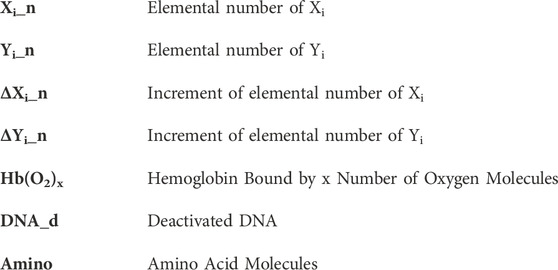
Initial element counts are necessary for computing the time evolution. X_i_n and Y_i_n are defined as the elemental number of X_i and Y_i; then, the following calculation in Equations 2, 3 with Equations 4, 5 provide the decrement and increment quantities of the elements.

$∆X_i\_n=-q_i\times R_{binomial}\left(n,p\right)(2)$

$∆Y_i\_n=r_i\times R_{binomial}\left(n,p\right)(3)$

$n={\mathit{int}\left(\frac{X_i\_n}{q_i}\right)}_{\mathit{min}}(4)$

$p=\prod _{i\ne \mathit{min}}\frac{k\bullet \left(\frac{X_i\_n}{q_i\bullet N}\right)}{1+k\bullet \left(\frac{X_i\_n}{q_i\bullet N}\right)}(5)$

R_binomial(n, p) generates random numbers following the binomial distribution, returning natural numbers (Rohr, 2018). In this function, n denotes a trial number, each of which can be either a success or a failure (binary outcomes). The parameter p specifies the probability of success in each trial. The function provides the total number of successes in n trials. NumPy’s random binomial (n, p) achieves this. The function returns one successful natural number under n, including zero. Stochastic simulation often uses these discrete numbers (Székely and Burrage, 2014; Gholami and Ilie, 2021). The trial number n is represented with the minimum integer value among X₁_n/q₁, X₂_n/q₂, X₃_n/q₃, so on. The probability p is derived based on the rate constant k, the reaction order q_i, a normalization parameter N, and X_i_n, except for $\frac{k\bullet \left(\frac{X_i\_n}{q_i\bullet N}\right)}{1+k\bullet \left(\frac{X_i\_n}{q_i\bullet N}\right)}$ with $\frac{X_i\_n}{q_i}$ selected in Equation 4. In a calculation step, X_i_n becomes X_i_n + ΔX_i_n and Y_i_n becomes Y_i_n + ΔY_i_n. The rate constant k in NNS is semantically the same as the rate constant that appears in the stoichiometric equation defined by concentration. However, k in this study is defined as a constant that affects the stochastic results defined in Equation 5. The rate constant k, the number of elements, and the normalization constant N determine the probability p, as indicated by Equation 5. The k value influences the probability variation between 0 and 1 and the reaction rate, but it is not the same as the conventional rate constant.

Equations 4, 5 have some minor formulas. One is in the case of a one-element reaction as Equation 6:

$\text{aX}\to r_1{Y}_1+r_2{Y}_2+\cdots +r_t{Y}_t\text{\hspace{0.17em}with\hspace{0.17em}}\mathrm{a}\text{\hspace{0.17em}rate\hspace{0.17em}constant\hspace{0.17em}}\mathrm{k}(6)$

X is a molecular element, and a is an order. The decrement ΔX_n and increment ΔY_i_n are derived from the following formulas as Equations 7, 8 with Equations 9, 10:

$∆X\_n=-a\times R_{binomial}\left(n,p\right)(7)$

$∆Y_i\_n=r_i\times R_{binomial}\left(n,p\right)(8)$

$\mathit{n}=\mathit{int}\left(\frac{\mathit{X}\_\mathit{n}}{\mathit{a}}\right)(9)$

$\mathit{p}=\frac{\mathit{k}}{\mathbf{1}+\mathit{k}}(10)$

where X_n is the number of the element X.

Another exceptional reaction type is as Equation 11:

$\mathbf{\text{aX\hspace{0.17em}}}\to \mathbf{0}\left(\text{zero}\right),\text{with\hspace{0.17em}}\mathrm{a}\text{\hspace{0.17em}rate\hspace{0.17em}constant\hspace{0.17em}}\mathrm{k}(11)$

This expression indicates that element X is decomposed and disappears, so Equation 3 does not work. Thus, only X decreases with Equation 7 with Equation 9, 10.

Another type of reaction is defined as a linear decreasing and increasing reaction for one element. One needs these reactions for the mathematical formulation of linear changes via molecular addition and subtraction. The linear decreasing case is defined similarly to Equation 11 as Equation 12:

$\text{aX\hspace{0.17em}}\to 0\left(\text{zero}\right)\text{\hspace{0.17em}by\hspace{0.17em}linear},\text{with\hspace{0.17em}}\mathrm{a}\text{\hspace{0.17em}rate\hspace{0.17em}constant\hspace{0.17em}}\mathrm{k}(12)$

Moreover, the increment of X is determined by the following Equation 13:

$∆\mathit{X}\_\mathit{n}=-\mathit{a}\times {\mathit{R}}_{\mathit{b}\mathit{i}\mathit{n}\mathit{o}\mathit{m}\mathit{i}\mathit{a}\mathit{l}}\left(\mathbf{1},\mathit{p}\right)(13)$

where p is the same as in Equation 10.

Subsequently, the linear increasing case is defined by the following reaction as Equation 14:

$\mathbf{0}\left(\mathit{z}\mathit{e}\mathit{r}\mathit{o}\right)\to \mathit{b}\mathit{Y}\text{\hspace{0.17em}by\hspace{0.17em}linear},\text{with\hspace{0.17em}}\mathrm{a}\text{\hspace{0.17em}rate\hspace{0.17em}constant\hspace{0.17em}}\mathrm{k}(14)$

The following Equation 15 also determines the increment of Y:

$∆\mathit{Y}\_\mathit{n}=\mathit{b}\times {\mathit{R}}_{\mathit{b}\mathit{i}\mathit{n}\mathit{o}\mathit{m}\mathit{i}\mathit{a}\mathit{l}}\left(\mathbf{1},\mathit{p}\right)(15)$

where p is the same as in Equation 10.

A biological system has numerous incredible reactions (Nelson and Cox, 2021). One can easily define each reaction if one knows the elements before and after the reaction, their orders, and rate constants.

Executing an input file in Spyder, an Integrated Development Environment requires setting “fName = “inp_file.txt”” in the main program (i.e., binomial_v016.py) and then utilizing the “Run” command. For command line execution, the command “$ python binomial_v016.py inp_file.txt” yields similar outcomes to Spyder’s run. Therefore, it is essential to position the input file in the program’s directory or one level above it.

This file needs to define calculation time, elements, reactions, and plots (Table 1). Currently, model systems are defined in text files. Currently, a Python program is available on GitHub that converts xml files that conform to Systems Biology Markup Language into text files for NNS. Users can perform calculations via NNS by setting the appropriate initial number of elements and rate constants.

Table 1

Table 1. Standard input file style. The *Time, *Element, *Reaction, and *Plot are commands for calculation in an input file.

The *Reaction statement has numerous definitions (Supplementary Tables S1, S2), including the above formulas used to calculate reaction increments.

The *ElementInOut statement implemented definition statements to express the inflow and outflow of molecules in and out of the system (Supplementary Table S3). The author developed the Python program used for this algorithm, and it is available under the MIT license on GitHub at https://github.com/taka-b/binomial/tree/binomial_v016_01 (Sato, 2023). This algorithm is publicly accessible and can be used by anyone without any charge. Figure 1A shows the calculation for schematic flow, while Figure 1B depicts the detailed calculation algorithm. The simplicity of the proposed procedure is demonstrated through six examples using their corresponding input files.

Figure 1

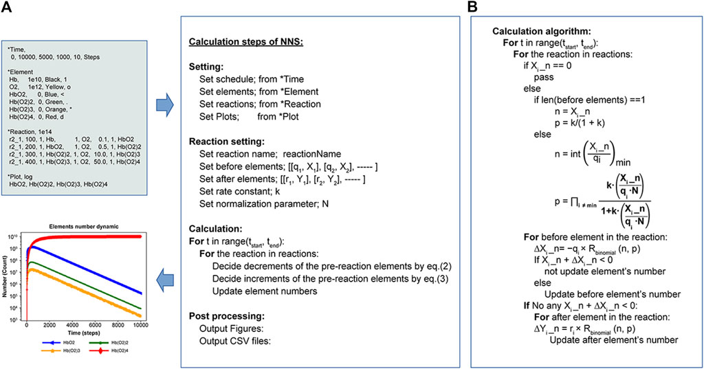
Figure 1. Calculation flow and algorithm of NNS. (A) Workflow executed by Python programs. The upper left shows an input file (Supplementary Figure S2A for an example), and the lower left depicts the resulting graph (Figure 5 for an example). (B) Detailed NNS calculation algorithm of the calculation in the Calculation steps of NNS: (A).

3 Results

Some example calculations are shown below. Note that the user only needs to prepare a text file for the calculations to obtain the results. The important point is to carefully formulate the stoichiometric equation and give appropriate rate constants.

The following results are obtained for calculations based on the text file shown in each figure. The start and end times are defined by *Time; for example, zero, 10,000, displays the results of calculations for every step from zero to 10,000. If you want to compare these results with actual experimental results, you will need units and rate constants that correspond to the experimental results. Here, however, the units of calculation are denoted in Steps, and figures show changes in the number of elements.

3.1 Simple reaction model

Consider a simple reaction with rate constant k_on as Equation 16:

$\mathit{A}+\mathit{B}\to \mathit{C},\text{with\hspace{0.17em}rate\hspace{0.17em}constant\hspace{0.17em}}{k}_{on}(16)$

where A and B represent protein molecules that irreversibly bind to form C.

Figure 2A is an input file (details in Table 1) defining one reaction r2_1_100 (details in Supplementary Table S1), where the calculation spans time zero to 10,000 in dimensionless units. In the actual calculation, each increase or decrease in the number of elements is calculated according to the above algorithm for each increase or decrease. The user must assign the appropriate time unit for a particular system. Here, for the sake of schematic calculation, the unit of time is used as the calculation unit Steps. NNS uses natural numbers, and as shown in Figure 2B, the y-axis represents the number of elements, guaranteeing an accurate number of elements.

Figure 2

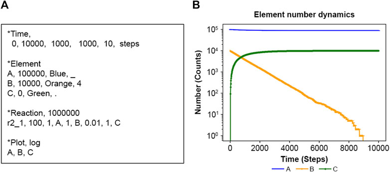
Figure 2. (A) Input text and (B) calculation result of (A).

In contrast, Supplementary Figure S1 introduces the inverse reaction r1_2_200 as Equation 17.

$\mathit{C}\to \mathit{A}+\mathit{B},\text{with\hspace{0.17em}rate\hspace{0.17em}constant\hspace{0.17em}}{\mathrm{k}}_{\text{off}}(17)$

The rate constant k_off differs from k_on in Equation 16 due to the thermodynamic principle in the system (Craig et al., 2021). Supplementary Figure S1 shows the equilibrium numbers of A, B, and C.

3.2 Water ionization

NNS can perform water ionization. Water, H₂O, usually dissociates slightly into proton ions (H⁺) and hydroxyl ions (OH⁻), representing a dynamical equilibrium between dissociation and reassociation. Figures 3A, B are input files in this scenario. Suitable rate constants show this equilibrium in Figures 3C, D. Notably, NNS accounts for system size through normalization parameters. Although the input files present different initial water molecule counts, their rate constants remain consistent. These normalization parameters adjust the system size by changing the success probability, p, in Equation 5. If a pseudo pH is defined as Equation 18:

$\mathit{p}\mathit{s}\mathit{e}\mathit{u}\mathit{d}\mathit{o}\mathit{p}\mathit{H}=-{\mathit{log}}_{\mathbf{10}}\left(\frac{\mathit{n}\mathit{u}\mathit{m}\mathit{b}\mathit{e}\mathit{r}\mathit{o}\mathit{f}\mathit{H}+}{\mathit{n}\mathit{u}\mathit{m}\mathit{b}\mathit{e}\mathit{r}\mathit{o}\mathit{f}\mathit{H}\mathbf{2}\mathit{O}}\right)(18)$

Figure 3

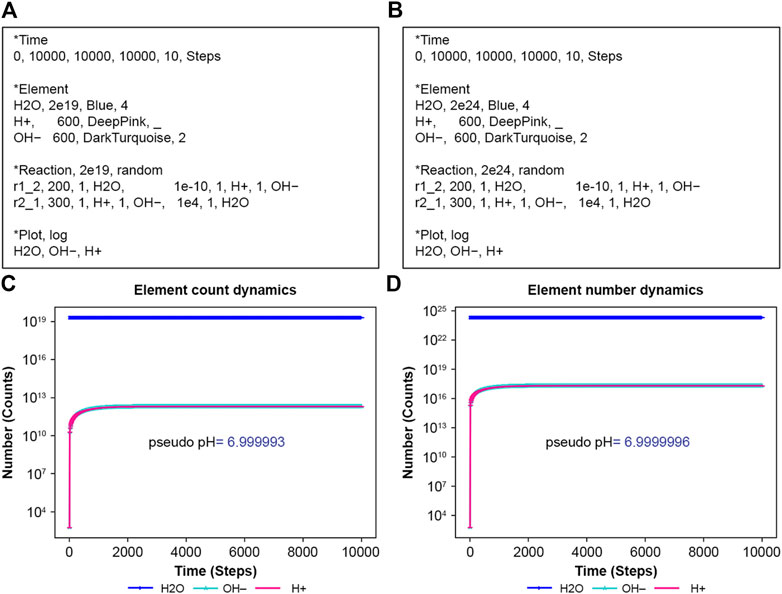
Figure 3. Ionization of water. H₂O means water, H₂O; H+ hydrogen ion H⁺; and OH–hydroxide ion, OH⁻. (A) Input text with N = 2e19 and (B) with N = 2e24. (C) The calculation result of (A,D) that of (B).

The results from Equation 18 using Figures 3B, D simulating data have almost the same values, 6.999993 and 6.9999996, respectively. The exact rate constants for the dissociation of water and recombination of proton ions (H⁺) and hydroxyl ions (OH⁻) remain unknown. Therefore, the horizontal axis in Figures 3C, D is labeled in Steps, the unit of calculation. If the exact values of these rate constants are known, the appropriate unit of time should be determined accordingly.

3.3 Michaelis–Menten model

Michaelis–Menten kinetics (Gilbert et al., 2006) is applied using NNS. In Figure 4A, E is an enzyme, S is the substrate, ES is the enzyme-substrate complex, and P is the product (Craig et al., 2021). The corresponding scheme is as Equation 19:

$\mathit{S}+\mathit{E}\rightleftarrows \mathit{E}\mathit{S}\to \mathit{E}+\mathit{P}(19)$

Figure 4

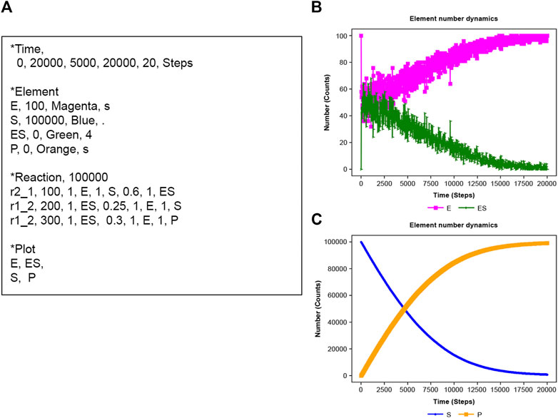
Figure 4. Michaelis–Menten kinetics. (A) Input text. (B) Results of E (enzyme) and ES enzyme-substrate complex). (C) Results of S (substrate) and P (product).

NNS defined three reactions in the input file. The total E number (E_n + ES_n) is constant, though E and ES fluctuate in time series (Figure 4B). Furthermore, S decreases with increasing P (Figure 4C).

3.4 Monod–Wyman–Changeux allosteric model

NNS can manage allosteric models (Goodey and Benkovic, 2008; Machado et al., 2015; Wodak et al., 2019). The allosteric transition of hemoglobin is one of the most interesting behaviors because of molecular adaptation in vertebrates (Eaton, 2022). Supplementary Figure S2A features an input file for the binding of oxygen to hemoglobin at different rate constants, 0.1, 0.5, 10, and 50. However, Supplementary Figure S2B uses a constant rate of 0.1. Figure 5A illustrates the allosteric effect; its increasing rate of oxyhemoglobin (Hb(O₂)₄) binding was higher than that observed in the no allosteric effect model of Figure 5B initially (Supplementary Figure S3A). The ratios of Hb(O₂)₄ to other complexes are also consistently higher than those observed in the non-allosteric model (Supplementary Figure S3B).

Figure 5

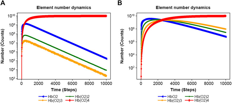
Figure 5. Results of the Monod–Wyman–Changeux allosteric model. (A) Result of Supplementary Figure S2A with rate constants: 0.1, 0.5, 10, and 50. (B) Result of Supplementary Figure S2B, with rate constants: 0.1, 0.1, 0.1, and 0.1.

3.5 Feedback loop model

NNS supports the models of feedback loops in biological systems, which are common regulatory mechanisms (Ferrazzi et al., 2011; Alon, 2019). Figure 6 depicts a feedback loop where a stimulus activates DNA, but the resultant protein then deactivates DNA into DNA_d (deactivated DNA). Supplementary Figure S4’s input file models ribonucleotide (Ribonucleotide) and amino acid (Amino) as singular types. The advantage of NNS is its ability to represent individual DNA molecules and deliver their specific properties. In Figure 7 the DNA is inactivated by the protein, mRNA production is stopped, and protein production is suppressed.

Figure 6

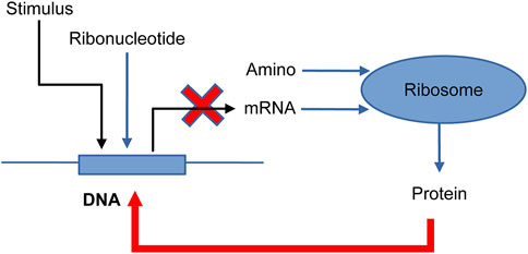
Figure 6. Feedback system model for one-gene DNA (Alon, 2019). Stimulus: protein molecules bind DNA; DNA: one gene; Ribonucleotide: some ribonucleotides; mRNA: messenger-RNA; Amino: some amino acids; Ribosome: ribosome for translation; and Protein: a protein made by the ribosome. DNA is transcribed into mRNA, which is then translated into Protein. The protein binds to DNA to deactivate and is modified into DNA_d (deactivate). (Reproduced from Alon, 2019, with permission from Chapman and Hall/CRC).

Figure 7

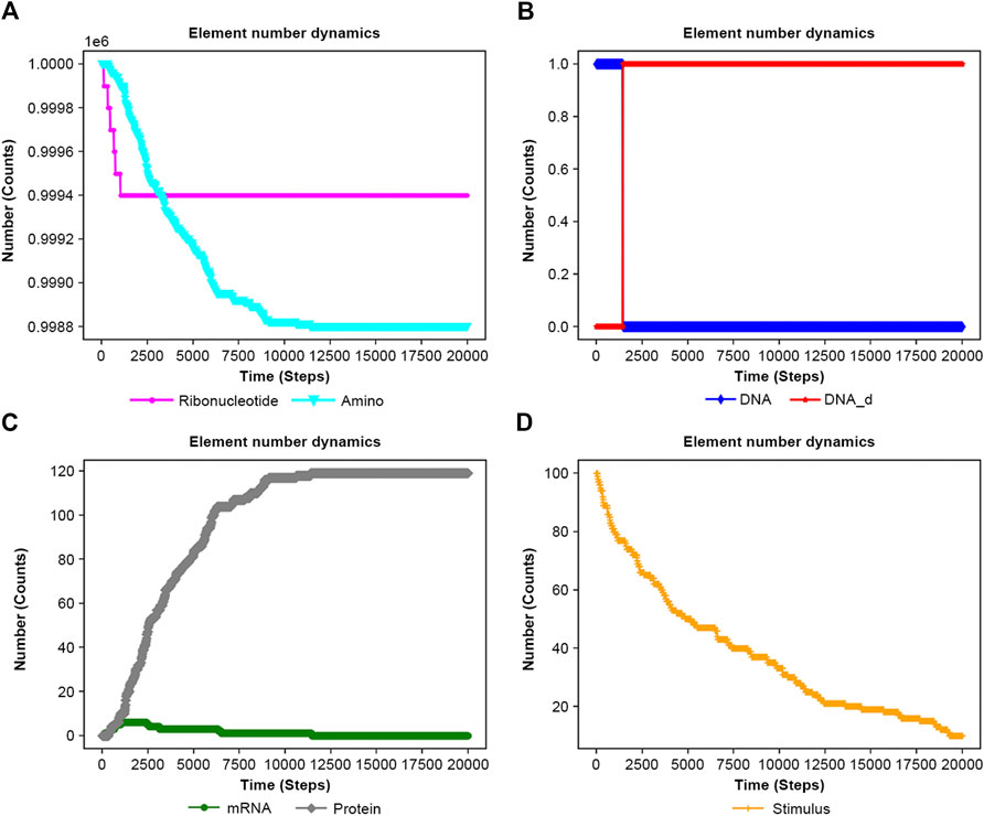
Figure 7. Results of the feedback system of the input file are in Supplementary Figure S4. (A) RNA and Amino. (B) DNA and DNA_d. (C) mRNA and Protein. (D) Stimulus.

Figure 7 and Supplementary Figure S5 exhibit contrasting results with and without feedback, respectively, highlighting the protein’s role in limiting DNA activation in feedback systems.

3.6 Feed-forward loop in a biological system

The feed-forward loop is a prevalent biological system (Kremling et al., 2008; Macía et al., 2009; Le and Kwon, 2011). Figure 8 depicts a schematic reaction process (Alon, 2019). Stimuli Sx and Sy ultimately promote protein pZ production. The system encompasses 10 elements, two input elements and six reactions, whose detailed functions are shown in the input file of Supplementary Figure S6. Using *elementInOut (Supplementary Table S3) and shifting the inflow timing of Sx and Sy as shown in Supplementary Figure S6 affects the behavior of the protein, as shown in Figure 9: Sy is inputted later than Sx, the production of Pz is delayed. On the other hand, in Supplementary Figures S7, S8, Sx and Sy are inputted simultaneously, there is no significant delay in Pz. The flexibility of NNS proves to be a valuable tool for modeling such a system.

Figure 8

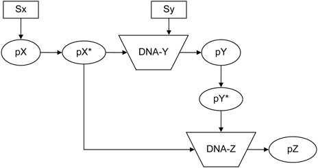
Figure 8. Feed-forward system (Alon, 2019). Sx and Sy: Stimuli; pX, pY, and pZ: proteins; pX* and pY*: activated proteins of pX and pY; DNA-Y and DNA-Z: DNA for each protein pY and pZ. (Reproduced from Alon, 2019, with permission from Chapman and Hall/CRC).

Figure 9

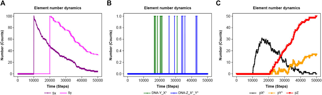
Figure 9. Results of the feed-forward system in Supplementary Figure S6 until time = 50,000 steps. Sx and Sy are added at 10,000 and 20,000 steps, respectively. (A) Sx and Sy. (B) DNA-Y_X* and DNA-Z_X*_Y*. (C) pX*, pY*, and pZ.

4 Discussion

Entropy and information are concepts related to information theory (Baez and Pollard, 2016), and stochastic processes with probability parameters can enrich our understanding of reaction systems. In our approach, parameters n and p are determined via reaction conditions and are described in the Methods section. The information on reaction is defined as Equation 20:

$\mathit{I}\_\mathit{r}\mathit{e}\mathit{a}\mathit{c}\mathit{t}\mathit{i}\mathit{o}\mathit{n}\left(\mathit{t},{\mathit{X}}_{\mathit{t}};{\mathit{n}}_{\mathit{t}},{\mathit{p}}_{\mathit{t}}\right)=-{\mathit{log}}_{\mathbf{2}}\left(\mathit{b}\mathit{i}\mathit{n}\mathit{o}\mathit{m}\mathit{i}\mathit{a}\mathit{l}\left({\mathit{X}}_{\mathit{t}};{\mathit{n}}_{\mathit{t}},{\mathit{p}}_{\mathit{t}}\right)\right)(20)$

where binomial ($X;n,p$) represents a binomial distribution function with a stochastic variable X (Successes) determined using n and p for each reaction step t (Chanda et al., 2020), as illustrated in Supplementary Figure S9.

The I_reaction provides insight into the reaction dynamics, and its value increases as reactions proceed.

Drawing from the Shannon entropy (Ben-Naim, 2012), the reaction entropy (RE) can be defined as Equation 21:

$\mathit{R}\mathit{E}\left(\mathit{t};{\mathit{n}}_{\mathit{t}},{\mathit{p}}_{\mathit{t}}\right)=-{\displaystyle \sum _{{\mathit{X}}_{\mathit{t}}=\mathbf{0}}^{{\mathit{n}}_{\mathit{t}}}}\mathit{b}\mathit{i}\mathit{n}\mathit{o}\mathit{m}\mathit{i}\mathit{a}\mathit{l}\left({\mathit{X}}_{\mathit{t}};{\mathit{n}}_{\mathit{t}},{\mathit{p}}_{\mathit{t}}\right){\mathit{log}}_{\mathbf{2}}\left(\mathit{b}\mathit{i}\mathit{n}\mathit{o}\mathit{m}\mathit{i}\mathit{a}\mathit{l}\left({\mathit{X}}_{\mathit{t}};{\mathit{n}}_{\mathit{t}},{\mathit{p}}_{\mathit{t}}\right)\right)(21)$

The RE is illustrated in Supplementary Figure S10 as a function of n and p, and it captures the inherent randomness in reaction and activity of reactions (Baez and Pollard, 2016; Roach, 2020; Uda, 2020).

Using a DNA-type reaction example from Figure 7 and Supplementary Figure S4, the accumulated information on the reaction is calculated using Equation 22.

$\mathit{I}{\mathit{R}}_{\mathit{a}\mathit{c}\mathit{c}\mathit{u}\mathit{m}\mathit{u}\mathit{l}\mathit{a}\mathit{t}\mathit{e}}\left(\mathit{t},{\mathit{X}}_{\mathit{t}};{\mathit{n}}_{\mathit{t}},{\mathit{p}}_{\mathit{t}}\right)=-{\displaystyle \sum _{{\mathit{t}}_{\mathit{k}}=\mathbf{0}}^{\mathit{t}}}{\mathit{log}}_{\mathbf{2}}\left(\mathit{b}\mathit{i}\mathit{n}\mathit{o}\mathit{m}\mathit{i}\mathit{a}\mathit{l}\left({\mathit{X}}_{{\mathit{t}}_{\mathit{k}}};{\mathit{n}}_{{\mathit{t}}_{\mathit{k}}},{\mathit{p}}_{{\mathit{t}}_{\mathit{k}}}\right)\right)(22)$

Figure 10 shows the results of Equation 22, and Figure 11 presents the RE values. Here, the RE values represent the results obtained from Equation 21 using Figure 7 and Supplementary Figure S4. Information on reaction and RE offers fundamental tools for dissecting reaction properties and understanding the complexity of biochemical systems.

Figure 10

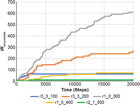
Figure 10. Accumulated information on the reaction was obtained using Equation 22 in the case of a feedback loop shown in Figure 7 and Supplementary Figure S3.

Figure 11

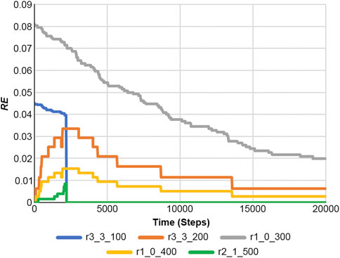
Figure 11. Reaction entropies of Equation 21 at any time in the case of a feedback loop of Figure 7 and Supplementary Figure S3.

Data availability statement

The datasets presented in this study can be found in online repositories. The names of the repository/repositories and accession number(s) can be found in the article/Supplementary Material.

Author contributions

TS: Conceptualization, Data curation, Formal Analysis, Software, Writing–original draft, Writing–review and editing.

Funding

The author(s) declare no financial support was received for the research, authorship, and/or publication of this article.

Acknowledgments

I want to thank my colleagues Kunihiko Oishi, Chika Morimoto, Minami Sakamoto, and Tatsuro Omori, who are all on my company team, for useful discussion.

Conflict of interest

Author TS was employed by Zeon Corporation.

Publisher’s note

All claims expressed in this article are solely those of the authors and do not necessarily represent those of their affiliated organizations, or those of the publisher, the editors and the reviewers. Any product that may be evaluated in this article, or claim that may be made by its manufacturer, is not guaranteed or endorsed by the publisher.

Supplementary material

The Supplementary Material for this article can be found online at: https://www.frontiersin.org/articles/10.3389/fcell.2024.1351974/full#supplementary-material

References

Adriaans, P., and van Benthem, J. (2008). Handbook of philosophy of information. Amsterdam: Elsevier Science Publishers.

Google Scholar

Alon, U. (2019). An introduction to system biology. 2nd ed. New York: Chapman and Hall/CRC.

Google Scholar

Baez, J. C., and Pollard, B. S. (2016). Relative entropy in biological systems. Entropy 18, 46. doi:10.3390/e18020046

CrossRef Full Text | Google Scholar

Baysoy, A., Bal, Z., Satija, R., and Fan, R. (2024). The technological landscape and applicatons of single-cell multi-omics. Nat. Rev. Mol. cell Biol. 24, 696–713. doi:10.1038/s41580-023-00615-w

CrossRef Full Text | Google Scholar

Ben-Naim, A. (2012). Entropy and the second law: interpretation and misss-interpretationsss teaneck. Singapore: World Scientific Publishing Inc.

Google Scholar

Blinov, M. L., Faeder, J. R., Goldstein, B., and Hlavacek, W. S. (2004). BioNetGen: software for rule-based modeling of signal transduction based on the interactions of molecular domains. Bioinformatics 20, 3289–3291. doi:10.1093/bioinformatics/bth378

PubMed Abstract | CrossRef Full Text | Google Scholar

Brinkrolf, C., Ochel, L., and Hofestädt, R. (2021). VANESA: an open-source hybrid functional Petri net modeling and simulation environment in systems biology. Biosystems 210, 104531. doi:10.1016/j.biosystems.2021.104531

PubMed Abstract | CrossRef Full Text | Google Scholar

Browning, A. P., Drovandi, C., Turner, I. W., Jenner, A. L., and Simpson, M. J. (2022). Efficient inference and identifiability analysis for differential equation models with random parameters. PLOS Comput. Biol. 18, e1010734. doi:10.1371/journal.pcbi.1010734

PubMed Abstract | CrossRef Full Text | Google Scholar

Chanda, P., Costa, E., Hu, J., Sukumar, S., Van Hemert, J., and Walia, R. (2020). Information theory in computational biology: where we stand today. Entropy (Basel) 22, 627. doi:10.3390/e22060627

PubMed Abstract | CrossRef Full Text | Google Scholar

Craig, N. L., Green, R. R., Greider, C. C., Wolberger, C., and Storz, G. G. (2021). “Molecular biology,” in Principles of genome function. 3rd ed (England: Oxford University Press).

CrossRef Full Text | Google Scholar

Eaton, W. A. (2022). A retrospective on statistical mechanical models for hemoglobin allostery. J. Chem. Phys. 157, 184104. doi:10.1063/5.0127585

PubMed Abstract | CrossRef Full Text | Google Scholar

Ferrazzi, F., Engel, F. B., Wu, E., Moseman, A. P., Kohane, I. S., Bellazzi, R., et al. (2011). Inferring cell cycle feedback regulation from gene expression data. J. Biomed. Inf. 44, 565–575. doi:10.1016/j.jbi.2011.02.002

PubMed Abstract | CrossRef Full Text | Google Scholar

Gholami, S., and Ilie, S. (2021). Reducing stochastic discrete models of biochemical networks. Appl. Math. 12, 449–469. doi:10.4236/am.2021.125031

CrossRef Full Text | Google Scholar

Gilbert, D., Fuss, H., Gu, X., Orton, R., Robinson, S., Vyshemirsky, V., et al. (2006). Computational methodologies for modelling, analysis and simulation of signalling networks. Brief. Bioinform. 7, 339–353. doi:10.1093/bib/bbl043

PubMed Abstract | CrossRef Full Text | Google Scholar

Gillespie, D. T. (1977). Exact stochastic simulation of coupled chemical reactions. J. Phys. Chem. 81, 2340–2361. doi:10.1021/j100540a008

CrossRef Full Text | Google Scholar

Goodey, N. M., and Benkovic, S. J. (2008). Allosteric regulation and catalysis emerge via a common route. Nat. Chem. Biol. 4, 474–482. doi:10.1038/nchembio.98

PubMed Abstract | CrossRef Full Text | Google Scholar

Gunawan, I., Vafaee, F., Meijering, E., and Lock, J. G. (2023). An introduction to representation learning for single-cell data analysis. Cell Rep. Methods 3, 100547. doi:10.1016/j.crmeth.2023.100547

PubMed Abstract | CrossRef Full Text | Google Scholar

Himeoka, Y., and Mitarai, N. (2022). Emergence of growth and dormancy from a kinetic model of the Escherichia coli central carbon metabolism. Phys. Rev. Research 4, 043233. doi:10.1103/PhysRevResearch.4.043223

CrossRef Full Text | Google Scholar

Huizing, G. J., Peyré, G., and Cantini, L. (2022). Optimal transport improves cell–cell similarity inference in single-cell omics data. Bioinformatics 38, 2169–2177. doi:10.1093/bioinformatics/btac084

PubMed Abstract | CrossRef Full Text | Google Scholar

Khodayari, A., and Maranas, C. D. (2016). A genome-scale Escherichia coli kinetic metabolic model k-ecoli457 satisfying flux data for multiple mutant strains. Nat. Commun. 7, 13806. doi:10.1038/ncomms13806

PubMed Abstract | CrossRef Full Text | Google Scholar

Kremling, A., Bettenbrock, K., and Gilles, E. D. (2008). A feed-forward loop guarantees robust behavior in Escherichia coli carbohydrate uptake. Bioinformatics 24, 704–710. doi:10.1093/bioinformatics/btn010

PubMed Abstract | CrossRef Full Text | Google Scholar

Le, D. H., and Kwon, Y. K. (2011). NetDS: a cytoscape plugin to analyze the robustness of dynamics and feedforward/feedback loop structures of biological networks. Bioinformatics 27, 2767–2768. doi:10.1093/bioinformatics/btr466

PubMed Abstract | CrossRef Full Text | Google Scholar

Lim, J., Park, C., Kim, M., Kim, H., Kim, J., and Lee, D. S. (2023). Advances in single-cell omics and multiomics for high-resolution molecular profiling. Exp. Mol. Med. 56, 515–526. doi:10.1038/s12276-024-01186-2

CrossRef Full Text | Google Scholar

Lin, X., Tian, T., Wei, Z., and Hakonarson, H. (2022). Clustering of single-cell multi-omics data with a multimodal deep learning method. Nat. Commun. 13, 7705. doi:10.1038/s41467-022-35031-9

PubMed Abstract | CrossRef Full Text | Google Scholar

Liu, F., Heiner, M., and Gilbert, D. (2023). Protocol for biomodel engineering of unilevel to multilevel biological models using colored Petri nets. STAR Protoc. 4, 102651. doi:10.1016/j.xpro.2023.102651

PubMed Abstract | CrossRef Full Text | Google Scholar

Machado, D., Herrgård, M. J., and Rocha, I. (2015). Modeling the contribution of allosteric regulation for flux control in the central carbon metabolism of E. coli. Front. Bioeng. Biotechnol. 3, 154. doi:10.3389/fbioe.2015.00154

PubMed Abstract | CrossRef Full Text | Google Scholar

Macía, J., Widder, S., and Solé, R. (2009). Specialized or flexible feed-forward loop motifs: a question of topology. BMC Syst. Biol. 3, 84. doi:10.1186/1752-0509-3-84

PubMed Abstract | CrossRef Full Text | Google Scholar

Massimino, M., Martorana, F., Stella, S., Vitale, S. R., Tomarchio, C., Manzella, L., et al. (2023). Single-cell analysis in the omics era: technologies and applications in cancer. Genes 14, 1330. doi:10.3390/genes14071330

PubMed Abstract | CrossRef Full Text | Google Scholar

Nelson, D. L., and Cox, M. M. (2021). Lehninger principles of biochemistry. 8th ed. New York: W. H. Freeman and Company.

Google Scholar

Roach, T. N. F. (2020). Use and abuse of entropy in biology: a case for caliber. Entropy (Basel) 22, 1335. doi:10.3390/e22121335

PubMed Abstract | CrossRef Full Text | Google Scholar

Rohr, C. (2018). Discrete-time leap method for stochastic simulation. Fundam. Inf. 160, 181–198. doi:10.3233/FI-2018-1680

CrossRef Full Text | Google Scholar

Ruths, D., Muller, M., Tseng, J. T., Nakhleh, L., and Ram, P. T. (2008). The signaling Petri net-based simulator: a non-parametric strategy for characterizing the dynamics of cell-specific signaling networks. PLOS Comput. Biol. 4, e1000005. doi:10.1371/journal.pcbi.1000005

PubMed Abstract | CrossRef Full Text | Google Scholar

Sato, T. (2023). Application of a novel numerical simulation to biochemical reaction systems. Available at: https://binomial-simulation.com/en/python (Accessed August 14, 2023).

Google Scholar

Shaikh, B., Smith, L. P., Vasilescu, D., Marupilla, G., Wilson, M., Agmon, E., et al. (2022). BioSimulators: a central registry of simulation engines and services for recommending specific tools. Nucleic Acids Res. 50, W108–W114. doi:10.1093/nar/gkac331

PubMed Abstract | CrossRef Full Text | Google Scholar

Shannon, C. E. (1948). A mathematical theory of communication. Bell Syst. Tech. J. 27, 379–423. doi:10.1002/j.1538-7305.1948.tb01338.x

CrossRef Full Text | Google Scholar

Székely, T., and Burrage, K. (2014). Stochastic simulation in systems biology. Comput. Struct. Biotechnol. J. 12, 14–25. doi:10.1016/j.csbj.2014.10.003

PubMed Abstract | CrossRef Full Text | Google Scholar

Uda, S. (2020). Application of information theory in systems biology. Biophys. Rev. 12, 377–384. doi:10.1007/s12551-020-00665-w

PubMed Abstract | CrossRef Full Text | Google Scholar

Ullah, M., and Wolkenhauer, O. (2011). Stochastic approaches for systems biology. New York: Springer.

Google Scholar

Wagle, M. M., Long, S., Chen, C., Liu, C., and Yang, P. (2024). Interpretable deep learning in single-cell omics. Bioinformatics 40, btae374. doi:10.1093/bioinformatics/btae374

PubMed Abstract | CrossRef Full Text | Google Scholar

Watson, J. D., Baker, T. A., Bell, S. P., Gann, A., Levine, M., and Losick, R. (2014). Molecular biology of the gene. 7th ed. London: Pearson.

Google Scholar

Wodak, S. J., Paci, E., Dokholyan, N. V., Berezovsky, I. N., Horovitz, A., Li, J., et al. (2019). Allostery in its many disguises: from theory to applications. Structure 27, 566–578. doi:10.1016/j.str.2019.01.003

PubMed Abstract | CrossRef Full Text | Google Scholar

Nomenclature