 Zahra Eidi1†
 Mehdi Sadeghi
95% of researchers rate our articles as excellent or good
Learn more about the work of our research integrity team to safeguard the quality of each article we publish.
Find out more
ORIGINAL RESEARCH article
Front. Cell Dev. Biol. , 30 July 2024
Sec. Morphogenesis and Patterning
Volume 12 - 2024 | https://doi.org/10.3389/fcell.2024.1310265
This article is part of the Research Topic Network-based Mathematical Modeling in Cell and Developmental Biology View all 10 articles
The spatial arrangement of variant phenotypes during stem cell division plays a crucial role in the self-organization of cell tissues. The patterns observed in these cellular assemblies, where multiple phenotypes vie for space and resources, are largely influenced by a mixture of different diffusible chemical signals. This complex process is carried out within a chronological framework of interplaying intracellular and intercellular events. This includes receiving external stimulants, whether secreted by other individuals or provided by the environment, interpreting these environmental signals, and incorporating the information to designate cell fate. Here, given two distinct signaling patterns generated by Turing systems, we investigated the spatial distribution of differentiating cells that use these signals as external cues for modifying the production rates. By proposing a computational map, we show that there is a correspondence between the multiple signaling and developmental cellular patterns. In other words, the model provides an appropriate prediction for the final structure of the differentiated cells in a multi-signal, multi-cell environment. Conversely, when a final snapshot of cellular patterns is given, our algorithm can partially identify the signaling patterns that influenced the formation of the cellular structure, provided that the governing dynamic of the signaling patterns is already known.
The duality of variety and organization is among the canonical concerns in biology. During the course of development in multicellular organisms, although successive cell divisions lead to the creation of diverse cells, it does not result in colony-like accumulation of piled-up cells. Although, in principle, the genetic material of every single cell of an organism is the same, influenced by variant stimulants, they are capable of generating highly complex spatial patterns (Liu and Warmflash, 2021; Dubrulle et al., 2015; Heemskerk et al., 2019; and van Boxtel et al., 2015). A diverse range of chemical stimuli, as underlying drivers of non-genetic variations, act at multiple scales (Shahbazi et al., 2019). These stimuli play a crucial role in directing cell fate determination in stem cells at the individual cell level (Britton et al., 2021). On the other hand, collective processes such as tissue homeostasis, wound healing, angiogenesis, and tumorigenesis are intimately linked with competing environmental chemical cues (Schweisguth and Corson, 2019). Understanding the mechanisms underlying the generation and maintenance of these ordered spatial assemblies could potentially aid in the development of novel strategies for controlling tissue organization and function in vitro and in vivo.During the development of multicellular organisms, tissues are created through the spatial arrangement of differentiated cells. Although modeling the formation of a spatial arrangement from a single stem cell is complex, it becomes even more complicated in reality as tissues are formed from the spatial arrangement of cells from different stem cells. This process requires intercellular signal transmission, which affects gene expression regulation and intracellular decision-making.Internal mechanisms are responsible for generating the right proportion of different types of specialized cells, distributing them in their right position, and maintaining the organized structure in the presence of intercellular chemical signaling agents (Khorasani and Sadeghi, 2022). Cells also sense and respond to mechanical stimuli and the physical properties of their environment via induced downstream genetic regulatory networks (Valet et al., 2022; Lenne et al., 2021; Wagh et al., 2021). Several multi-stable regulatory networks play their role as the internal decision-makers of dividing cells (Khorasani and Sadeghi, 2022). This study investigates the impact of various chemical signals on the mechanism by which multiple stem cells generate intricate tissue structures and tries to provide a deeper understanding of the mechanisms behind morphological variations. In reality, the formation of intermediate structures during embryo development or the formation of a tissue consisting of cells with different phenotypes and with organization in their spatial arrangement without a previous template is a complex problem, and modeling them using the simplest possible assumptions can lead to a better comprehension of the development process in multicellular organisms.We would like to answer these questions, or, more realistically, get any enlightenment about the following: first, in the presence of variant positional cues, how can spatially organized populations give rise to and maintain large-scale inhomogeneities starting from an initially roughly homogeneous mass of intermixed stem cell populations? Second, how do individual stem cells perceive and interpret their surrounding spatial information to make decisions about their developmental pathway in response to the local concentration of these stimulants? Finally, is it possible to infer information about the specific form of the signals that created them from the final structure of cell populations?
The basis of cellular pattern formation is mounted on the interaction of the mediating nonlinear diffusive signaling components (Murray, 2001). For the spontaneous construction of patterns during development, as proposed by Turing’s classic theory, the system requires two diffusive chemical compounds: an activator compound and an inhibitor compound (Turing, 1990). The latter locally undergoes an autocatalytic reaction to generate more of itself and also activates the formation of the inhibitor compound in some way. Meanwhile, the former inhibits the formation of more activator compounds. The key element for obtaining spatial patterns is that the activator and the inhibitor components diffuse through the reaction medium at different rates. Thus, the effective ranges of their respective influences are different. Accordingly, if the inhibitor agent diffuses faster than the activator one, a stable pattern can emerge from a homogeneous background merely by the amplification of small perturbations. The patterns generally take the form of spots (and reverse spots) or stripes based on the choice of model parameters (Murray, 2001). The dynamic elaborates different possible pattern formation processes in a variety of developmental situations. The related examples span from the regeneration of hydras (Meinhardt, 2003) to animal coating patterns (Koch and Meinhardt, 1994). Wave phenomena can also generate patterns of spatiotemporal type (Cotterell et al., 2015; Eidi et al., 2021). Since the typical characteristic time of cell division is higher than that of a traveling wave, here, we exclude the formation of cellular patterns induced by spatiotemporal signaling patterns. Recently, Marcon et al. (2016) proposed a new development in classical Turing models, indicating that the essential prerequisite of varied diffusion rates for mobile signaling molecules is not essential for pattern formation. Remarkably, specific networks are capable of creating patterns using signals without the constraint of relative diffusion rates.
Here, we assume that there are two multipotent stem cells as resources of variation generation, each of which is potentially capable of constructing its own organized structure in the absence of the other. Although the cells do not directly interact, they have an intracellular signal-dependent tri-stable switch that affects their reproduction rates in response to multiple signals in the environment. We present a computational model for their internal mechanism in the presence of each other to form an organized population consisting of whole descendants. We see that signaling messengers play a significant and irreplaceable role as regulatory agents in communication between different cell types. Our results indicate that the association of variant environmental signaling messengers and intracellular decision-making switches grants a diverse range of cellular patterns. Furthermore, having the ultimate arrangement of cellular organization, one can approximately indicate the signaling patterns based on which the cellular patterns have been established, provided that the prior assumption of the pattern is given.
In this model, we consider a scenario where a plane is initially populated by two types of stem cells,
The materials and methods is structured as follows: first, we introduce different possible dynamics for propagating extracellular signals in the environment, including positional information in Section 2.1.1 and reaction–diffusion dynamics in Section 2.1.2. Subsequently, in Section 2.2, we propose a regulatory switch that allows an individual cell to determine its fate influenced by the uptake of different environmental signals. Finally, in Section 2.3, we describe an algorithm for predicting the final cellular pattern of a system that is initially composed of multiple signaling agents and dividing cells.
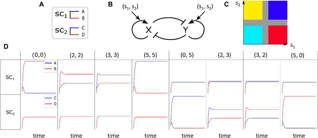
Figure 1. Fate determination of stem cells under the influence of environmental signaling agents. (A) Differentiation of
Let us assume that the stem cells in a medium are exposed to spatial chemical information, we refer to them as signals, which are captured and interpreted by the cells to develop the spatial organization. There are various ways to provide spatial patterns in biology, among which, positional information and reaction–diffusion dynamics are the most prominent (Green and Sharpe, 2015).
Generally, positional information dynamic refers to the development of the spatial cellular organization in the embryo differentiating at specific positions based on their response to the gradient of environmental signals (Schweisguth and Corson, 2019). For example, embryonic organizer centers secrete morphogens that specify the emergence of germ layers and the establishment of the body’s axes during embryogenesis (De Santis et al., 2021). In the current study, by positional information, we mean any external chemical cues whose procedure of setting up is immaterial for us, and we merely focus on their impact on the regulation of internal switches. To illustrate the relationship between different signals, Figure 2 exemplifies the simultaneous presence of two signal profiles of Gaussian type (the first column), a Gaussian profile and a sinusoidal one (the second and third columns), and two sinusoidal with different frequencies (the fourth column). In each column, the final cellular pattern resulting from the process of cell division and self-renewal of competing stem cells is represented by the third row. Initially, the stem cells are randomly distributed in an environment that contains upper-row signals. In all cases, the final pattern can be distinguished by six different colors. The colors magenta and green represent
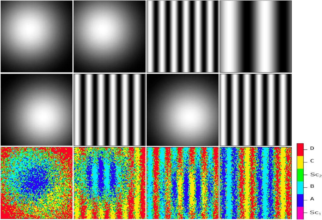
Figure 2. Resulting cellular pattern (third row) of a system influenced by two independent static signal profiles (first and second rows). The signal profiles consist of a Gaussian profile, described by the exponential function
To generate two independent signaling agents in the medium, we consider a system that consists of two independent reaction–diffusion processes. Each process involves two interacting chemicals, namely,
Here, by rescaling the space variable, the diffusion coefficient of
Here,
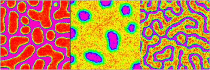
Figure 3. Possible signaling agent patterns
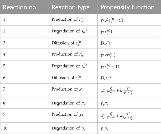
Table 1. Involved reactions and their corresponding propensity functions (reaction no. 1–6) generating signaling patterns and the reactions (reaction no. 7–10) involved in the production and degradation of intracellular determinants. In total, there are 20 reactions incorporated in the Gillespie algorithm,
As previously mentioned, we assume that the concentration field of
Once we have identified the environmental signals that can influence the fate of stem cells, we can explore the subsequent question: how do simultaneous signals impact the destiny of a single cell?
Let us assume that within the cytoplasm of each stem cell
In Figure 1B, the regulatory switch is shown. It involves mutual repression of
It has been demonstrated by Khorasani et al. (2020) that in the absence of stimulant signaling chemicals, when there is only one type of stem cell and the coefficients in Equations 3, 4 are constant, there are three stable steady-states for each stem cell. These steady states correspond to three distinct cell fates: the stem cell itself and its corresponding differentiated cells. The cell’s absorption to a specific attractor is determined by the values of
Here,
In this section, we introduce a position-dependent procedure based on the Gillespie algorithm to simulate the development of differentiated cells in a population, as illustrated in Figure 4. The Gillespie algorithm is widely used for modeling systems with a small number of determinants or chemicals, taking into account inherent fluctuations. Previous studies have mainly focused on understanding the decision-making mechanism of a single type of stem cell. However, in this study, we extend our analysis to include multiple types of stem cells and various signaling stimulants in the system.
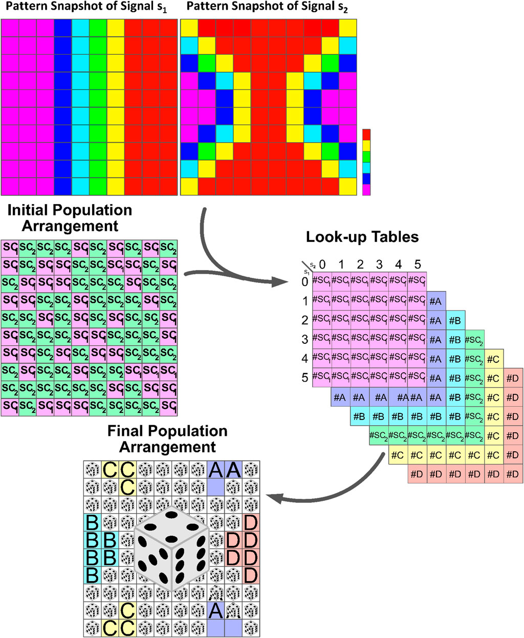
Figure 4. Schematic illustration of the formation of developmental patterns influenced by external signals. Stem cells respond to dynamic signals, leading to differentiation and self-renewal based on the number of determinants produced within their cytoplasm. Look-up tables summarize cell division outcomes based on the signal combination intervals. The highlighted section with dice in the lower panel represents regions with comparable signal concentrations. Here, the response of stem cells to these signals becomes unpredictable, and randomness plays an important role in determining the outcome. See Algorithm 1 for in-depth details.
Consider a system comprising two types of stem cells, namely,
The cell cycle span represents the average time interval in which each stem cell reaches the domain of one of its possible attractors: the stem cell itself or its differentiated offspring. Through trial and error, it has been determined that approximately 100 steps are necessary for the cells to reach a state of homeostasis. During this period, the values of intercellular signaling agents and intracellular determinants are updated using the Gillespie algorithm. Table 1 contains the list of reactions for these variants along with their corresponding propensity functions. Once this period is completed, the cells are ready to undergo division. At this point, we record the probable number of each possible fate based on the values of the signals and determinants. These numbers serve as the “virtual” destination of the stem cells and are recorded in their respective
The process then repeats for another cell cycle duration, which is typically 100 steps. After collecting enough data in the look-up tables, for example after 1,000 steps, we can estimate the probability (Pb) of each of the six cell types being born. This is done by referring to the look-up tables and calculating the probability as the number of that particular cell type in the table divided by the total population size.
The entire process continues until the difference between two successive Pb values becomes smaller than a predefined tiny value, denoted as
To simulate the dynamic of the pattern formation through the division process provoked by the positional chemical information, we perform the following steps recurrently on a substrate of size
1. For an adequate duration, such as 100 successive steps, let the dynamic of Equations 3, 4, upon which the number of determinant agents evolves, proceed. Here, we reckon that the signaling patterns of
2. Follow up the “potential” destiny of the stem cell located at each grid on the plane. Allocate a
3. Repeat the two previous steps 1,000 times, and record the corresponding classified data according to the above-mentioned method. In this way, one collects more data and, in consequence, the final predicted fate of the cells is closer to that of a real system.
4. Once every 1000 steps, assess the amount of
5. Finally, substitute the initial distribution of mother cells
In a population of stem cells, the number of dividing cells remains constant. An alternative explanation for the above algorithm can be described as follows: once the mother cells reach a state of homeostasis after 100 steps, they divide. However, the algorithm disregards the differentiated cells as the algorithm focuses on studying the internal switch of the stem cells at this stage. Thus, we assume that only the stem cell daughter cells remain at each grid point. In the next iteration, the offspring stem cells explore the phase space of
The only additional assumption in this description is that every division always yields a stem cell as its daughter cell. The difference between the two descriptions lies in the fact that the first description defines potential cell fates, while the latter assumes that the divisions are real. Both descriptions aim to gather more data, resulting in a final predicted fate of the cells that are closer to that of a real system.
Figure 1D illustrates the solutions of Equations 3, 4 in the presence of variant pairs of
Algorithm 1.The sequential instruction to form a complex cellular pattern based on a given signaling blueprint.
To ensure a sufficient number of iterations, the initial value of
Construct the medium and plant stem cells,
Form signal patterns s1 and s2.
while
for
Update the system.
end
Let the stem cells be divided potentially, observe the offspring, and collect the data.
if
end
end
Design the corresponding medium based on the collected data
Figure 5 depicts the arrangement of the final developed cellular patterns induced as a result of variant possible combinations of signaling patterns governed by Eqs 1, 2. The color bar represents different cell types. Purple and green stand for
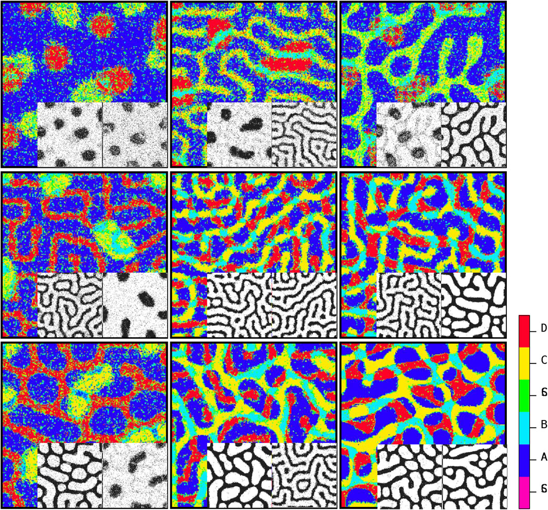
Figure 5. Steady-state patterns of developmental cellular arrangements in a multiple signaling field. The figures depict the patterns obtained using Algorithm 1, with each pattern governed by the dynamics of Equations 1, 2. The inline patterns, shown alongside, correspond to the signaling patterns predicted by Algorithm 2. By understanding the distribution of stimulating signals for stem cells, Algorithm 1 can determine the final cellular developmental pattern. Conversely, the inline patterns are generated according to the guidelines outlined in Algorithm 2 by analyzing the steady-state cellular pattern in each element as input. The color code reflects the cell types.
Algorithm 2.The sequential instructions for determining the form of triggering signaling patterns (spot, reverse spot, or stripe) associated with the final cellular arrangement in a system of two reproducing stem cells (
for
for
if
end
if
end
if
end
if
end
if
end
if
end
end
end
Figure 5 depicts the ultimate configurations of cellular arrangements resulting from different combinations of signaling patterns generated by Eqs 1, 2. The two corresponding acquired signaling patterns are displayed at the bottom right of each array. The key point here is that there is a dual relationship between the signal distribution and cell growth pattern. By understanding the distribution of signals that stimulate stem cells, algorithm 1 can be utilized to ascertain the final cell growth pattern. Conversely, by knowing the specific types of signals present, algorithm 2 can be employed to determine the parameters associated with the signal pattern based on the final cellular arrangement. In other words, if we are provided with a snapshot of the steady state of a developed cellular pattern and we assume that this pattern is influenced by two independent signals (s1 and s2) generated through a Turing process with Eqs 1, 2, algorithm 2 can predict the shape of each signal (spot, reverse spot, or stripe) based on the observed final cellular pattern. Recognition of signal patterns is a directional process. Algorithm 2: first, it is necessary to consider two blank planes, each of which is in accord with one of the signals to project its corresponding pattern onto it. Next, we go through every single pixel of the cellular pattern. Then, based on the color of the pixel, we map the projection of this color onto the signal planes. Let us assume that the color of a pixel is blue, meaning that this pixel is occupied with a cell of phenotype
The positional stimuli have been emerging as key regulators of transcription and gene expression in diverse physiological contexts (Rulands et al., 2018). These environmental drivers engage in the phenotypic diversity and proliferation/differentiation balance of stem cells (Balázsi et al., 2011; Rulands and Simons, 2016; Blake et al., 2006). The regulation process of non-genetic diversity involves the interplay of intracellular and intercellular components to interpret positional cues (Çağatay et al., 2009; Acar et al., 2008). In a competing arena in which various chemical stimulants vie for affecting a cell’s fate more, the process demands more robust and complex mechanisms. In order to specify and extend their offspring territory, the stem cells utilize a signaling process to communicate and collaborate with each other. This process ends in collective self-organized forms on length scales that are much larger than those of the individual units Chhabra et al. (2019).
In this study, first, we investigated the impact of multiple passive external signals on intracellular switches of a single stem cell. This provides us with a direct inspection of the connection between intracellular and extracellular dynamics. By mapping the environmental signaling patterns to the probability of the emergence of differentiated cell types, this model is capable of capturing any desired complex pattern, whether passive or active. The sort of models that recapitulates signaling dynamics and predicts cell fate patterning upon chemical perturbations precedingly has been investigated in non-competitive environments (Khorasani and Sadeghi, 2022; Khorasani et al., 2020; Sharifi-Zarchi et al., 2015; Chambers et al., 2007; Kalmar et al., 2009; Chen et al., 2010; Bergsmedh et al., 2011). Here, we focused on the behavior of each cell in the interaction with multiple signals. Figure 2 illustrates the resulting phenotypic cellular patterns of different combinations of two typical signal profiles of Gaussian and sinusoidal blueprints.
The environmental signals influence the fate of each stem cell, SCi (i = 1,2), by means of biasing the regulation of our tri-stable switch; see Equations 3, 4. Based on the definition of
After investigating the impact of static environmental stimulants on the internal switch, we dealt with the active signaling between the sources that produce variant phenotypes. We took advantage of confined Turing models for two different signals secreted from each of stem cells (Shoji et al., 2003). The dynamic includes linear reaction terms and additional constraints that confine the two variables within a finite range. The resulting patterns of this dynamic are either stationary striped patterns or spotted patterns. The second pattern, in turn, consists of two forms: spotted and reverse spotted patterns. Here, the tuning parameter upon which the pattern type is specified is the maximum concentration of the activator
Stochasticity has been proven to be a non-genetic diversifying resource of variation in nature (Delbrück, 1940; McEntire et al., 2021; Acar et al., 2008; Kepler and Elston, 2001; Wu and Tzanakakis, 2012; Perez-Carrasco et al., 2016). It has been shown that controlled amount of randomness ends in phenotypic variation and, as a result, population heterogeneity (Losick and Desplan, 2008; Greulich and Simons, 2016; Khorasani et al., 2020). In this study, to reflect the non-deterministic portion of the signaling system, we implemented the Gillespie algorithm (Gillespie et al., 2007) by stepping in time to successive molecular reaction events according to the premises of the model of Shoji et al. (2003); see Equations 1, 2. Another aspect of incorporating randomness in our reductionist insight is simulating the emergence of every cell type in the look-up table based on the calculation of its corresponding probability; see Figure 4. Stochastic algorithms generally provide the chance to explore multiple solutions and potentially uncover a better one compared to a deterministic method, which may get stuck in a local minimum (Gillespie et al., 2007). Additionally, these algorithms can be easily tailored to different problems and constraints, making them adaptable for solving more complex issues. By utilizing stochastic methods, we can account for the inherent randomness and fluctuations present in natural systems. This strategy allows for controlled noise to be introduced into the system. As long as the level of randomness is controllable, the system’s behavior remains predictable, and the resultant patterns are statistically reproducible.
In our algorithm, we evaluate the similarity between cellular patterns exposed to different pairs of signaling patterns by comparing them numerically to a cellular pattern constructed through a deterministic process while being exposed to the same pair of signaling patterns. This measure of similarity serves as an indicator of the reproducibility of cellular patterns using the algorithm proposed. To accomplish this, we first create two new
By using these extreme signaling patterns, we can determine the fate of each stem cell in the medium and create a deterministic cellular pattern accordingly. We now have a reference pattern to assess the reproducibility of our algorithm and measure the resemblance of different patterns exposed to similar pairs of signaling patterns. Figure 6 illustrates five different realizations for various pairs of signaling patterns. The signaling patterns are shown above each column, and the resulting cellular population realizations are displayed below them in each column. We can compare each realization with its corresponding deterministic pattern, pixel by pixel. If the cell types in a pixel are identical, we assign a score of
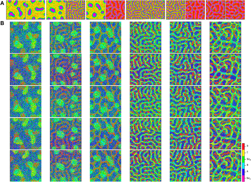
Figure 6. Comparison of cellular patterns for multiple pairs of signaling patterns simulated using the proposed algorithm. Panel (A) illustrates the signaling patterns pairs at the top of each column, while Panel (B) shows five independent simulated cellular patterns for each pair. The apparent similarity of the cellular patterns demonstrates the reproducibility of the method. Refer to Figure 7 for an analytical measure of the pattern similarity.

Figure 7. Box plot illustrating the normalized score values for the cellular patterns depicted in Figure 6. The score value measures the similarity of each pattern to a reference deterministic pattern created from their extreme signaling value pairs.
In conclusion, this study demonstrates that the signal-dependent tri-stable switch can serve as a useful tool to bridge intracellular dynamics with intercellular structures. In this scenario, although the stem cells do not directly interact with each other, their reproduction rates are influenced by external signals in their environment through the switch mechanism within each cell. By studying individual cellular decisions and the influence of multiple signals, we observe how complex cellular patterns emerge. Although the algorithm utilized in this study simplifies certain aspects, such as considering the dynamic environment during cell division, apoptosis, and cell movement, the presented systematic approach allows for the simulation of complex cellular organizations based on fundamental biophysical processes, resulting in reproducible outcomes. Moreover, for any given complex cellular pattern, for which merely the prior class of signal patterns is known, the provided method closely concludes the signaling profile that sets off the cellular pattern. Overall, these findings highlight the potential of using signal-dependent switches for better comprehension and regulation of cellular behaviors in diverse scenarios.
The original contributions presented in the study are included in the article/Supplementary Material; further inquiries can be directed to the corresponding author.
ZE: conceptualization, formal analysis, investigation, methodology, validation, visualization, and writing–original draft. NK: conceptualization, formal analysis, investigation, methodology, software, validation, visualization, and writing–review and editing. MS: conceptualization, methodology, project administration, validation, and writing–review and editing.
The author(s) declare that no financial support was received for the research, authorship, and/or publication of this article.
The authors declare that the research was conducted in the absence of any commercial or financial relationships that could be construed as a potential conflict of interest.
All claims expressed in this article are solely those of the authors and do not necessarily represent those of their affiliated organizations, or those of the publisher, the editors, and the reviewers. Any product that may be evaluated in this article, or claim that may be made by its manufacturer, is not guaranteed or endorsed by the publisher.
Acar, M., Mettetal, J. T., and Van Oudenaarden, A. (2008). Stochastic switching as a survival strategy in fluctuating environments. Nat. Genet. 40, 471–475. doi:10.1038/ng.110
Balázsi, G., Van Oudenaarden, A., and Collins, J. J. (2011). Cellular decision making and biological noise: from microbes to mammals. Cell 144, 910–925. doi:10.1016/j.cell.2011.01.030
Bergsmedh, A., Donohoe, M. E., Hughes, R.-A., and Hadjantonakis, A.-K. (2011). Understanding the molecular circuitry of cell lineage specification in the early mouse embryo. Genes 2, 420–448. doi:10.3390/genes2030420
Blake, W. J., Balázsi, G., Kohanski, M. A., Isaacs, F. J., Murphy, K. F., Kuang, Y., et al. (2006). Phenotypic consequences of promoter-mediated transcriptional noise. Mol. Cell 24, 853–865. doi:10.1016/j.molcel.2006.11.003
Britton, G., Chhabra, S., Massey, J., and Warmflash, A. (2021). “Fate-patterning of 2d gastruloids and ectodermal colonies using micropatterned human pluripotent stem cells,” in Programmed morphogenesis (Springer), 119–130.
Çağatay, T., Turcotte, M., Elowitz, M. B., Garcia-Ojalvo, J., and Süel, G. M. (2009). Architecture-dependent noise discriminates functionally analogous differentiation circuits. Cell 139, 512–522. doi:10.1016/j.cell.2009.07.046
Chambers, I., Silva, J., Colby, D., Nichols, J., Nijmeijer, B., Robertson, M., et al. (2007). Nanog safeguards pluripotency and mediates germline development. Nature 450, 1230–1234. doi:10.1038/nature06403
Chen, L., Wang, D., Wu, Z., Ma, L., and Daley, G. Q. (2010). Molecular basis of the first cell fate determination in mouse embryogenesis. Cell Res. 20, 982–993. doi:10.1038/cr.2010.106
Chhabra, S., Liu, L., Goh, R., Kong, X., and Warmflash, A. (2019). Dissecting the dynamics of signaling events in the bmp, wnt, and nodal cascade during self-organized fate patterning in human gastruloids. PLoS Biol. 17, e3000498. doi:10.1371/journal.pbio.3000498
Cotterell, J., Robert-Moreno, A., and Sharpe, J. (2015). A local, self-organizing reaction-diffusion model can explain somite patterning in embryos. Cell Syst. 1, 257–269. doi:10.1016/j.cels.2015.10.002
Delbrück, M. (1940). Statistical fluctuations in autocatalytic reactions. J. Chem. Phys. 8, 120–124. doi:10.1063/1.1750549
De Santis, R., Etoc, F., Rosado-Olivieri, E. A., and Brivanlou, A. H. (2021). Self-organization of human dorsal-ventral forebrain structures by light induced shh. Nat. Commun. 12, 6768–6811. doi:10.1038/s41467-021-26881-w
Dubrulle, J., Jordan, B. M., Akhmetova, L., Farrell, J. A., Kim, S.-H., Solnica-Krezel, L., et al. (2015). Response to nodal morphogen gradient is determined by the kinetics of target gene induction. Elife 4, e05042. doi:10.7554/eLife.05042
Eidi, Z., Khorasani, N., and Sadeghi, M. (2021). Reactive/less-cooperative individuals advance population’s synchronization: modeling of dictyostelium discoideum concerted signaling during aggregation phase. PloS one 16, e0259742. doi:10.1371/journal.pone.0259742
Gallagher, K. D., Mani, M., and Carthew, R. W. (2022). Emergence of a geometric pattern of cell fates from tissue-scale mechanics in the drosophila eye. Elife 11, e72806. doi:10.7554/eLife.72806
Gillespie, D. T., et al. (2007). Stochastic simulation of chemical kinetics. Annu. Rev. Phys. Chem. 58, 35–55. doi:10.1146/annurev.physchem.58.032806.104637
Green, J. B., and Sharpe, J. (2015). Positional information and reaction-diffusion: two big ideas in developmental biology combine. Development 142, 1203–1211. doi:10.1242/dev.114991
Greulich, P., and Simons, B. D. (2016). Dynamic heterogeneity as a strategy of stem cell self-renewal. Proc. Natl. Acad. Sci. 113, 7509–7514. doi:10.1073/pnas.1602779113
Heemskerk, I., Burt, K., Miller, M., Chhabra, S., Guerra, M. C., Liu, L., et al. (2019). Rapid changes in morphogen concentration control self-organized patterning in human embryonic stem cells. Elife 8, e40526. doi:10.7554/eLife.40526
Kalmar, T., Lim, C., Hayward, P., Munoz-Descalzo, S., Nichols, J., Garcia-Ojalvo, J., et al. (2009). Regulated fluctuations in nanog expression mediate cell fate decisions in embryonic stem cells. PLoS Biol. 7, e1000149. doi:10.1371/journal.pbio.1000149
Kepler, T. B., and Elston, T. C. (2001). Stochasticity in transcriptional regulation: origins, consequences, and mathematical representations. Biophysical J. 81, 3116–3136. doi:10.1016/S0006-3495(01)75949-8
Khorasani, N., and Sadeghi, M. (2022). A computational model of stem cells’ decision-making mechanism to maintain tissue homeostasis and organization in the presence of stochasticity. Sci. Rep. 12, 9167–9217. doi:10.1038/s41598-022-12717-0
Khorasani, N., and Sadeghi, M. (2024). A computational model of stem cells' internal mechanism to recapitulate spatial patterning and maintain the self-organized pattern in the homeostasis state. Sci. Rep. 14, 1528–1615. doi:10.1038/s41598-024-51386-z
Khorasani, N., Sadeghi, M., and Nowzari-Dalini, A. (2020). A computational model of stem cell molecular mechanism to maintain tissue homeostasis. Plos one 15, e0236519. doi:10.1371/journal.pone.0236519
Koch, A., and Meinhardt, H. (1994). Biological pattern formation: from basic mechanisms to complex structures. Rev. Mod. Phys. 66, 1481–1507. doi:10.1103/revmodphys.66.1481
Lenne, P.-F., Munro, E., Heemskerk, I., Warmflash, A., Bocanegra-Moreno, L., Kishi, K., et al. (2021). Roadmap for the multiscale coupling of biochemical and mechanical signals during development. Phys. Biol. 18, 041501. doi:10.1088/1478-3975/abd0db
Liu, L., and Warmflash, A. (2021). Self-organized signaling in stem cell models of embryos. Stem Cell Rep. 16, 1065–1077. doi:10.1016/j.stemcr.2021.03.020
Losick, R., and Desplan, C. (2008). Stochasticity and cell fate. science 320, 65–68. doi:10.1126/science.1147888
Marcon, L., Diego, X., Sharpe, J., and Müller, P. (2016). High-throughput mathematical analysis identifies turing networks for patterning with equally diffusing signals. Elife 5, e14022. doi:10.7554/eLife.14022
McEntire, K. D., Gage, M., Gawne, R., Hadfield, M. G., Hulshof, C., Johnson, M. A., et al. (2021). Understanding drivers of variation and predicting variability across levels of biological organization. Integr. Comp. Biol. 61, 2119–2131. doi:10.1093/icb/icab160
Meinhardt, H. (2003). Models of biological pattern formation: common mechanism in plant and animal development. Int. J. Dev. Biol. 40, 123–134.
Murray, J. D. (2001). Mathematical biology II: spatial models and biomedical applications, 3. New York: Springer.
Omid-Shafiei, S., Hassan, M., Nu¨ssler, A. K., Najimi, M., and Vosough, M. (2023). A shadow of knowledge in stem cell science. Cell J. (Yakhteh) 25, 738–740. doi:10.22074/cellj.2023.2005680.1346
Perez-Carrasco, R., Guerrero, P., Briscoe, J., and Page, K. M. (2016). Intrinsic noise profoundly alters the dynamics and steady state of morphogen-controlled bistable genetic switches. PLoS Comput. Biol. 12, e1005154. doi:10.1371/journal.pcbi.1005154
Rulands, S., Lescroart, F., Chabab, S., Hindley, C. J., Prior, N., Sznurkowska, M. K., et al. (2018). Universality of clone dynamics during tissue development. Nat. Phys. 14, 469–474. doi:10.1038/s41567-018-0055-6
Rulands, S., and Simons, B. D. (2016). Tracing cellular dynamics in tissue development, maintenance and disease. Curr. Opin. Cell Biol. 43, 38–45. doi:10.1016/j.ceb.2016.07.001
Schweisguth, F., and Corson, F. (2019). Self-organization in pattern formation. Dev. Cell 49, 659–677. doi:10.1016/j.devcel.2019.05.019
Shahbazi, M. N., Siggia, E. D., and Zernicka-Goetz, M. (2019). Self-organization of stem cells into embryos: a window on early mammalian development. Science 364, 948–951. doi:10.1126/science.aax0164
Sharifi-Zarchi, A., Totonchi, M., Khaloughi, K., Karamzadeh, R., Araúzo-Bravo, M. J., Baharvand, H., et al. (2015). Increased robustness of early embryogenesis through collective decision-making by key transcription factors. BMC Syst. Biol. 9, 23–16. doi:10.1186/s12918-015-0169-8
Shoji, H., Iwasa, Y., and Kondo, S. (2003). Stripes, spots, or reversed spots in two-dimensional turing systems. J. Theor. Biol. 224, 339–350. doi:10.1016/s0022-5193(03)00170-x
Staff, P. C. B. (2017). Correction: intrinsic noise profoundly alters the dynamics and steady state of morphogen-controlled bistable genetic switches. PLOS Comput. Biol. 13, e1005563. doi:10.1371/journal.pcbi.1005563
Turing, A. (1990). The chemical basis of morphogenesis. B. Jack Copel. 52, 153–197. doi:10.1007/BF02459572
Valet, M., Siggia, E. D., and Brivanlou, A. H. (2022). Mechanical regulation of early vertebrate embryogenesis. Nat. Rev. Mol. Cell Biol. 23, 169–184. doi:10.1038/s41580-021-00424-z
van Boxtel, A. L., Chesebro, J. E., Heliot, C., Ramel, M.-C., Stone, R. K., and Hill, C. S. (2015). A temporal window for signal activation dictates the dimensions of a nodal signaling domain. Dev. Cell 35, 175–185. doi:10.1016/j.devcel.2015.09.014
Wagh, K., Ishikawa, M., Garcia, D. A., Stavreva, D. A., Upadhyaya, A., and Hager, G. L. (2021). Mechanical regulation of transcription: recent advances. Trends Cell Biol. 31, 457–472. doi:10.1016/j.tcb.2021.02.008
Keywords: developmental pattern, signaling, cell tissue, self-organization, regenerative therapy, Turing dynamics
Citation: Eidi Z, Khorasani N and Sadeghi M (2024) Correspondence between multiple signaling and developmental cellular patterns: a computational perspective. Front. Cell Dev. Biol. 12:1310265. doi: 10.3389/fcell.2024.1310265
Received: 09 October 2023; Accepted: 02 July 2024;
Published: 30 July 2024.
Edited by:
Susan Mertins, Leidos Biomedical Research, Inc., United StatesReviewed by:
Romas Baronas, Vilnius University, LithuaniaCopyright © 2024 Eidi, Khorasani and Sadeghi. This is an open-access article distributed under the terms of the Creative Commons Attribution License (CC BY). The use, distribution or reproduction in other forums is permitted, provided the original author(s) and the copyright owner(s) are credited and that the original publication in this journal is cited, in accordance with accepted academic practice. No use, distribution or reproduction is permitted which does not comply with these terms.
*Correspondence: Mehdi Sadeghi, c2FkZWdoaUBuaWdlYi5hYy5pcg==
†These authors have contributed equally to this work
Disclaimer: All claims expressed in this article are solely those of the authors and do not necessarily represent those of their affiliated organizations, or those of the publisher, the editors and the reviewers. Any product that may be evaluated in this article or claim that may be made by its manufacturer is not guaranteed or endorsed by the publisher.
Research integrity at Frontiers
Learn more about the work of our research integrity team to safeguard the quality of each article we publish.