 Ashwath Kumar
 Michael Y. Hu
 Yajun Mei3,4
 Yuhong Fan
94% of researchers rate our articles as excellent or good
Learn more about the work of our research integrity team to safeguard the quality of each article we publish.
Find out more
ORIGINAL RESEARCH article
Front. Cell Dev. Biol., 25 May 2023
Sec. Epigenomics and Epigenetics
Volume 11 - 2023 | https://doi.org/10.3389/fcell.2023.1167111
Chromatin immunoprecipitation followed by sequencing (ChIP-seq) has revolutionized the studies of epigenomes and the massive increase in ChIP-seq datasets calls for robust and user-friendly computational tools for quantitative ChIP-seq. Quantitative ChIP-seq comparisons have been challenging due to noisiness and variations inherent to ChIP-seq and epigenomes. By employing innovative statistical approaches specially catered to ChIP-seq data distribution and sophisticated simulations along with extensive benchmarking studies, we developed and validated CSSQ as a nimble statistical analysis pipeline capable of differential binding analysis across ChIP-seq datasets with high confidence and sensitivity and low false discovery rate with any defined regions. CSSQ models ChIP-seq data as a finite mixture of Gaussians faithfully that reflects ChIP-seq data distribution. By a combination of Anscombe transformation, k-means clustering, estimated maximum normalization, CSSQ minimizes noise and bias from experimental variations. Further, CSSQ utilizes a non-parametric approach and incorporates comparisons under the null hypothesis by unaudited column permutation to perform robust statistical tests to account for fewer replicates of ChIP-seq datasets. In sum, we present CSSQ as a powerful statistical computational pipeline tailored for ChIP-seq data quantitation and a timely addition to the tool kits of differential binding analysis to decipher epigenomes.
Epigenetics causes heritable phenotypes without alterations in the DNA sequence. Histone modifications and chromatin binding proteins are among the most prevalent epigenetic modifications that define epigenomes (Allis and Jenuwein, 2016). ChIP-seq, chromatin immunoprecipitation followed by sequencing, has revolutionized the study of protein-DNA interaction in vivo, enabling genome-wide profiling of histone modifications and the localization of chromatin binding proteins (Johnson et al., 2007; Park, 2009). Massive amounts of ChIP-seq data have been generated, illuminating versatile epigenomes that shed light on the mechanisms of epigenetic gene regulation (Mundade et al., 2014; Hollbacher et al., 2020). However, the complexity and variability of ChIP-seq experiments have made quantitative comparisons among ChIP-seq datasets challenging.
In ChIP-seq assay, DNA-protein complexes are immunoprecipitated with antibodies specific for proteins of interest, followed by deep sequencing of the immunoprecipitated DNA. Sequencing reads are aligned to the reference genome. Individual ChIP-seq data has been primarily used to identify DNA regions enriched for the occupancy of chromatin binding proteins or histone modifications within the genome through finding “peaks,” i.e., DNA regions enriched with sequence reads by immunoprecipitation. A number of “peak finding” bioinformatics tools, such as MACS (Zhang et al., 2008) and SICER (Zang et al., 2009), have been developed and benchmarked (Jeon et al., 2020). While identification of peak regions has dramatically increased our understanding of epigenomes, it remains important to capture the rich quantitative metrics of signal intensities that are critical for tracking quantitative and comparative changes in epigenomes among different samples, and the demand for bioinformatics tools that faithfully capture the full expressivity of ChIP-seq data are increasingly (Nakato and Sakata, 2021; Zhao and Chen, 2021). Thus, to harness the full value of ChIP-seq data, it is imperative to develop statistically robust pipelines to expand the tool kits for identification and quantification of differential binding (DB) in epigenomes.
Current pipelines for DB detection from ChIP-seq datasets can be broadly classified into two groups (Steinhauser et al., 2016; Tu and Shao, 2017; Eder and Grebien, 2022): one group, as exampled in DiffBind (Ross-Innes et al., 2012), ChIPComp (Chen et al., 2015) and DBChIP (Liang and Keles, 2012), utilizes peak-calling algorithms to define peak regions followed by statistical tests to identify DB regions among the peak regions; the other group, such as diffReps (Shen et al., 2013), PePr (Zhang et al., 2014), and CSAW (Lun and Smyth, 2016), performs genome-wide analysis to identify all possible DB regions. DiffBind and CSAW have been shown to have top performance in their respective categories (Stark and Brown, 2011; Ross-Innes et al., 2012; Lun and Smyth, 2016; Eder and Grebien, 2022). Both DiffBind and CSAW adopt negative binomial models that have been successfully used in popular statistical packages, such as DESeq2 (Love et al., 2014) and edgeR (Robinson et al., 2010), for differential gene expression analysis of RNAseq data. However, due to the overall lower signal/noise ratios of ChIP-seq as compared with RNAseq, compounded by the significant variations of signal intensities and coverage among ChIP-seq datasets by using different protocols, antibodies, or experimental efficiency, extending the statistical methodology developed for RNAseq analysis to ChIP-seq poses challenges. In addition, it is critical for the interpretation of ChIP-seq results to include proper parallel control experiments, such as sequencing of input or non-specific IgG ChIP-seq, for which data distribution does not optimally fit negative binomial model. Further, to maximize the value of ChIP-seq, it is important to detect and quantify differential binding for any designated regions, regardless of peak or non-peak regions. Thus, to develop statistical tools that allow robust comparisons of signal intensities among different ChIP-seq datasets, we must go back to the data and rebuild our modeling choices from scratch.
Here, we have developed a statistically robust pipeline, ChIP-seq Signal Quantifier (CSSQ), uniquely tailored for quantitative analysis of ChIP-seq datasets, capable of comparisons across different experiments for any designated genomic regions. In this pipeline, we adopt a Gaussian mixture model for transformed data instead of directly modeling raw count or discrete data. This method is robust because we first transform count data to continuous data whose distribution can then be approximated arbitrarily well by a finite mixture of Gaussian distributions (McLachlan and Peel, 2000). Specifically, we first process ChIP-seq data using the variance-stabilizing Anscombe transformation (Anscombe, 1948), followed by fitting a Gaussian mixture model through the use of k-means clustering, and finally scaling the dataset by estimated maximum value normalization. This approach effectively mitigates background noise and biases associated with individual experimental differences. Such pre-processed ChIP-seq data is implemented for statistical analysis using a non-parametric method suitable for small sample sizes to detect and quantify DBs. Benchmarking studies by extensive computational simulations and experimentally validated real ChIP-seq datasets demonstrate the robustness and sensitivity of CSSQ in detection and quantification of DBs. In addition to its distinctive features in handling varied signal/noise ratios prevalent in ChIP-seq datasets, CSSQ allows incorporation of input/IgG control datasets and offers superior performance and statistical power with as little as two replicates per group.
Genome aligned BAM files or raw sequence reads FASTQ files of ChIP-seq and RNA-seq datasets (Supplementary Table S1) were downloaded from the source and processed (Consortium, 2011; Shen et al., 2012; Geeven et al., 2015). Raw sequencing reads of FASTQ files were quality checked using FastQC (Andrews, 2022), trimmed using TrimGalore (Martin, 2011; Krueger, 2021).
Trimmed sequence reads from ChIP-seq datasets were aligned to human or mouse genomes (as listed in Supplementary Table S1) using bowtie v1.1.2 (Langmead et al., 2009) to obtain BAM files as described previously (Cao et al., 2013). Aligned BAM files were sorted using SAMtools (Li et al., 2009) and reads within predefined regions were counted using Bedtools (Quinlan and Hall, 2010). For ChIP-seq datasets, both Chromatin Immunoprecipitated-seq data (IP) and its control chromatin Input-seq data (IN) were counted. The sum of sequence depth normalized counts of each pre-defined region was obtained as their corresponding IP and IN signals. Background subtracted ChIP-seq signals, as defined as (IP-IN), were calculated.
Trimmed sequence reads from RNA-seq were aligned to genomes using STAR aligner (Dobin et al., 2013), quantified using HTSeq (Anders et al., 2015), and analyzed for differential gene expression using the DESeq2 R package (Love et al., 2014). The Ensembl v75 annotation for human genome and RefSeq annotation for mouse genome were used to obtain gene locations and promoter regions.
For each pre-defined region, Anscombe transformation, defined by
The simulated datasets were generated based on H3K4me3 ChIP-seq datasets from H1 hESCs (GSM733657 and GSM733770 of GSE29611 series). The simulated datasets were generated as follows. The ChIP-seq signals of a real dataset were processed to obtain (IP-IN)* signals and served as the base dataset. For each simulation, four statistically similarly simulated datasets were created to have the same data distribution as the base dataset to mimic the null hypothesis of no differences between the datasets, named as Sim1#-Sim4#. Specially, the base (IP-IN)* dataset was split into two normal distributions with one covering the “L” cluster and the other covering the “M,” “H,” and “S” clusters. The mean and variance of each of these two normal distributions of the base dataset were used to generate simulated (IP-IN)#sim datasets from randomly created values that fit into the same data distribution using truncated normal distribution method. The number of data points, the minimum and maximum values of each cluster were maintained for each corresponding cluster of all initial simulated datasets (Sim1#-Sim4#). In addition, randomly picked simulated data points in “L” cluster were converted to 0 to ensure the level of zero inflation maintained as the base dataset from real datasets.
For DB induction (DBI), data points of randomly selected regions from the 3rd and 4th initial simulated datasets were induced to change values with varying or fixed (2–6) times the SD of the corresponding cluster of the selected regions. In addition, (IP-IN)*sim values were constrained between 0 and 1 to avoid outliers. Each simulated dataset was subsequently multiplied by a Usim, a value randomly sampled from a Kernel Density Estimate fitted from the estimated maximum values (U) of 20 real ChIP-seq datasets, to create corresponding (IP-IN)Asim datasets (Sim1A- Sim4A), followed by reversed Anscombe transformation to derive corresponding simulated (IP-IN)sim datasets (Sim1-Sim4). For each simulation condition, a total of 300 simulation runs were performed on 300 independently generated sets of simulation datasets with 1 run/simulation dataset (of Sim1-4 datasets).
DB analysis using DiffBind, CSAW, and CSSQ were performed as follows.
DiffBind v2.8.0 (Ross-Innes et al., 2012): Aligned bam files of ChIP-seq datasets and the coordinates of the regions of interest in bed format were fed to DiffBind for analysis. “dba.count,” “dba.contrast” and “dba.analyze” functions were used to perform differential binding analysis. For these functions, the “minMembers” parameter was set to 2 to indicate the number of replicates, and the method was set to use DESeq2 available within DiffBind. An FDR cutoff of 0.05 was used to identify significant DB regions. For simulated datasets, DBA objects were created from (IP-IN)sim values, followed by DB analysis.
CSAW v1.14.0 (Lun and Smyth, 2014; Lun and Smyth, 2016): Aligned bam files of ChIP-seq datasets and the coordinates of the regions of interest in bed format were fed into CSAW for analysis. The “regionCount,” “windowCounts,” “filterWindowsGlobal,” and “normOffsets” functions within CSAW were used to quantify and normalize signal over regions of interest. To fit the quasi-likelihood model and perform statistical tests, CSAW uses the “asDGEList,” “estimateDisp,” “glmQLFit,” “glmQLFTest,” “mergeWindows,” and “combineTests” functions. An FDR of 0.05 was used to identify significant DB regions. For simulated datasets, “RangedSummarizedExperiment” objects were created from (IP-IN)sim values, followed by DB analysis.
CSSQ: Aligned bam files were used to quantify the number of reads that overlap the regions of interest using Bedtools (Quinlan and Hall, 2010). Depth normalized IP-IN signals were subsequently derived by subtraction of normalized read counts of ChIP-seq sample by that of its input-seq sample for each of the predefined regions. All negative IP-IN values were converted to 0. This pre-processed IP-IN data points were fed to CSSQ for Anscombe transformation, normalization, k-means clustering and DB analysis using a non-parametric statistical test. Regions that had IP-IN values above zero in one or more datasets were kept for subsequent analysis. An FDR cutoff of 0.05 was used to filter for significant DBs.
Hierarchical clustering of regions was performed using MeV (Howe et al., 2011) and Metagene analyses were performed using GenPlay genome analyzer and browser (Lajugie and Bouhassira, 2011; Lajugie et al., 2015). The signal intensity of 100bp sliding windows covering the entire defined region were plotted. Aligned bam files were used to quantify the number of reads in each window for each sequencing dataset. The counts for each dataset were normalized to 10 million mappable reads. IP-IN signals were subsequently derived by subtraction of normalized read counts of ChIP-seq (IP) dataset by that of its corresponding input-seq (IN) dataset for each window.
CSSQ integrates data pre-processing, transformation, and parameter estimation in a Gaussian mixture model (clustering, normalization) and statistical test, enabling vigorous DB detection and quantification (Figure 1A). To develop a statistically robust pipeline, we first evaluated the data distribution of representative ChIP-seq signals (Figure 1B, Supplementary Figure S1). For sample ChIP-seq datasets of H3K4me3, an active histone mark enriched at active gene promoters (Barski et al., 2007; Heintzman et al., 2007; Jambhekar et al., 2019), the sum of sequence depth normalized counts covering a 2-kb promoter region centered around transcription start site (TSS) of each gene was calculated for H3K4me3 ChIP-seq data (IP) and its control chromatin Input-seq data (IN) to obtain their corresponding IP and IN signals. Negative IP-IN values that reflected regions with signals below background noise were converted to 0 to enhance data visualization and to facilitate downstream statistical transformations. The overall data distribution of IP-IN exhibited similar patterns to IP, with high concentration of values around 0 followed by a wide range of data points with mixed multi-modal distribution patterns (Figure 1B, Supplementary Figure S1).
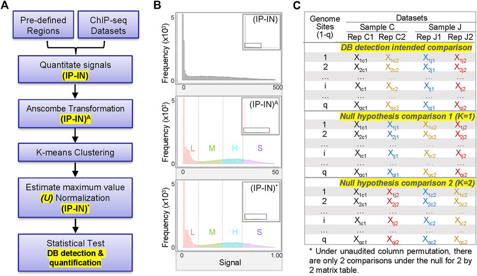
FIGURE 1. Overview of CSSQ pipeline. (A) Flow chart of CSSQ pipeline. (B) Representative histograms of H3K4me3 ChIP-seq datasets throughout CSSQ pipeline. Zoomed out histograms are shown as insets. (IP-IN)A: Anscombe transformed data. (IP-IN)*: CSSQ normalized values. L, M, H, S clusters are derived from k-means clustering and color coded as pink, green, blue, and purple, respectively. (C) Representative matrix table of datasets for DB detection using CSSQ.
To have a better model on the distribution of complex data for optimal statistical pipeline development, we fit a mixture model instead of a single distribution. To be more specific, we transformed the raw, discrete ChIP-seq count data to continuous values so that statistical analysis using Gaussian mixture distributions is feasible. Among the various widely used transformation approaches for transformation of non-Gaussian to Gaussian data or Gaussian mixture models, based on our extensive numerical experience, we chose the Anscombe transformation for its variance stabilizing properties and suitability for both small and large values (Anscombe, 1948). The Anscombe transformation is defined by
Next, we estimated the parameters of the Gaussian mixture model through k-means clustering (McLachlan and Peel, 2000) with the goal of normalizing disparate datasets to an equal scale via an estimated maximum normalization approach. This is crucial for DB identification and quantification across datasets because individual ChIP-seq datasets often differ substantially in their data distribution and range of signal intensities, even for replicate datasets from the same biological sample (Figure 1B, Figure 2, Supplementary Figure S1). To robustly compute the estimated maximum value (designated as “U” factor), we first utilized the k-means clustering algorithm to partition data points into k = 4 clusters representing categories of low (L), medium (M), high (H) and super (S) signal intensities (Figure 1B, Figure 2). Data points within each k cluster have minimal in-cluster variances and thus are considered as within the same Gaussian distribution. The mean and variance of each cluster were calculated to estimate the parameters of the corresponding components in the Gaussian mixture model. The cluster with the largest mean (S cluster) was used to derive the value of U, defined as
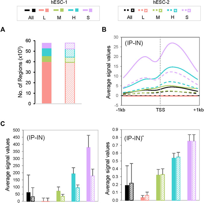
FIGURE 2. Characterization of CSSQ clusters. (A) Cluster allocations of datapoints of two representative datasets of H3K4me3 ChIP-seq of hESCs. (B) Metagene analysis of H3K4me3 ChIP-seq signals centered around transcription start sites (TSS). (C) Bar charts of mean ChIP-seq signal values pre- (left) and post- (right) CSSQ normalization. Error bars: standard deviation.
To detect and quantify DBs, CSSQ uses a statistical test based on the Welch’s two-sample t-statistic for data points of each row/region. The difference between the comparisons was calculated as follows:
where
Given the q observed test statistics
For example, of representative datasets shown in Figure 1C, whereas nc = 2, nj = 2, n = nc + nj = 4, z will be 2 as calculated:
The p-value for each row/region is subsequently defined using the following formula:
Next, we applied the Benjamini–Hochberg correction to pi (Benjamini and Hochberg, 1995) to compute adjusted p-values for the i-th row (pi-adj) to select statistically significant DB regions (Figure 1). Finally, a fold-change (FC) is calculated for DBs by using the average of the different groups following the equation below.
Due to the absence of a gold standard for quantitative analysis of differential binding, we employed computational simulations to test CSSQ performance. Simulation studies enable induction of true positive (TP) DBs with varying magnitude and scope, allowing comparisons of CSSQ with parallel pipelines, CSAW and DiffBind, for benchmarking performance. We devised a scheme to create simulated datasets that resemble real datasets with true DB induction (DBI) (Figure 3, Supplementary Figure S4, Methods). For each simulated experiment, an q ∗ n matrix where q is the number of regions and n is the total number of datasets (n = 4 represented in Figure 1C) was generated, including two hypothetical replicates of the two samples (designated as C, J) for comparisons.
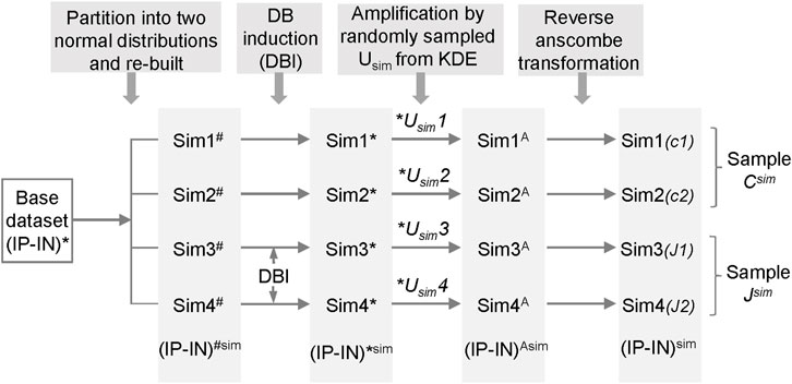
FIGURE 3. The scheme for generating simulated datasets.
To generate each simulated dataset of Sim1-4, a base (IP-IN)* dataset derived from a real dataset was partitioned into two normal distributions from which parameters were extracted to re-build a simulated base dataset of Sim1-4# with randomized numbers. DBs were induced in Sim3-4# on randomly selected data points by changing values with varying or fixed (2–6) times the standard deviation (SD) of the corresponding cluster of the selected regions. The obtained 4 datasets, named as Sim1-4*, were then each amplified by a Usim factor randomly sampled from the Kernel Density Estimate (KDE) curve fitted and based on U factors calculated from real ChIP-seq datasets (Supplementary Figure S2). The resulting datasets, designated as Sim1-4A, were reverse Anscombe transformed to produce corresponding Sim1-4 datasets (Figure 3). Using this approach, we produced simulated datasets with data distribution mimicking real datasets (Supplementary Figures S1, S4).
We next scanned the performance of CSSQ, CSAW and DiffBind using Sensitivity (defined as true DBs detected/induced DBs), False Discovery Rate (FDR) (defined as false DBs detected/total DBs detected), and the receiver operating characteristic (ROC) curves as metrics. We utilized two base datasets, hESC-1 and hESC-2 H3K4me3 ChIP-seq datasets, to create two series of simulation datasets and performed simulation runs in parallel to gauge the robustness of each pipeline with datasets of different data distribution patterns (Supplementary Table S1, Supplementary Figure S1A). A total of 7,800 simulations were performed to test the effects of varying the percentages of the data points as DBI and of varying the magnitudes of changes of DBI (Figure 4, Methods). Among the three pipelines, CSSQ displayed the highest sensitivity in DB detection in all simulation conditions of both SimhESC-1 and SimhESC-2 series (Figure 4). CSSQ and CSAW had consistently low FDR, and CSSQ also exhibited superior performance in ROC curves with Area Under the Curve (AUC) higher than 0.95 in all simulations, consistently ranked the highest among three tools in all scenarios, indicating that CSSQ outperforms CSAW and DiffBind in differentiating true (induced) and false (non-induced) DBs (Figure 4, Supplementary Figure S5).
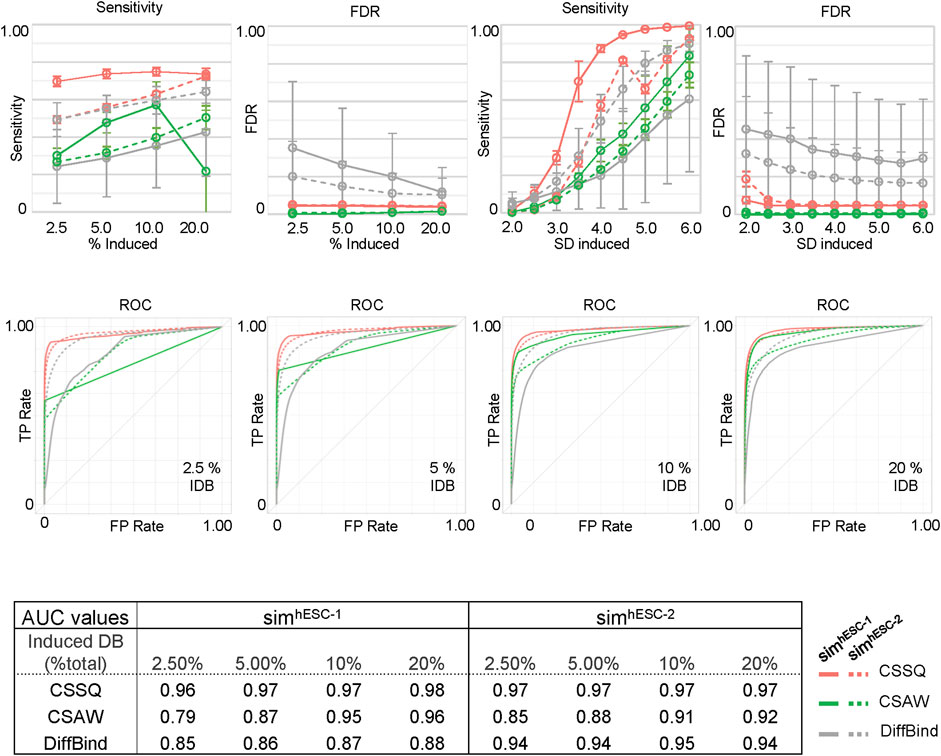
FIGURE 4. DB detection and quantitation on simulated datasets using CSSQ and parallel methods. Sensitivity, FDR, ROC curves and AUC values of DB detection are shown. Each spot averaged results from 300 simulation analyses with each simulation generated a set of four datasets based on real H3K4me3 ChIP-seq datasets of hESC-1 or hESC-2. DBs were induced by either alteration of variable (2–6)* SD on randomly selected data points on indicated % of data points or with fixed multiplier of SD on 2.5% data points of the data points. ROC curves and the values of Area Under the Curve (AUC) for DB detection of induced DBs by addition or reduction of values using variable SD method on randomly selected 2.5%, 5%, 10% and 20% of datapoints are shown. IDB: induced DBs. Error bars: SD.
On our benchmarks, CSSQ also outperformed CSAW and DiffBind by in depth analysis of detected DBs against induced DBs (TP). We scrutinized the DBs detected by the three pipelines from two representative sets of 4 simulated datasets, each of simhESC-1 and simhESC-2 (Figure 5, Supplementary Figure S6). CSSQ DBs had the closest clustering pattern as that of the true DBs, and CSSQ consistently detected the highest number and percentage of true DBs with very low % of false positive calls (Figure 5A, 5B, Supplementary Figure S6). In the simhESC-1 sample analysis, 1,420 DBs were induced with 81% being up DBs. CSSQ detected 1,035 of TP DBs, whereas CSAW and DiffBind only detected 408 and 329 TP DBs, supporting the superior sensitivity of CSSQ in DB detection (Figure 5B). Further, CSSQ detected 82% of DBs upregulated, closely mimicking DBI; whereas CSAW and DiffBind had fewer, 58% and 32%, of DBs as upregulated (Figure 5). DB partition into clusters indicated that CSSQ DBs had cluster distribution closely matching DBI while CSAW and DiffBind DBs deviated significantly from TP DBs (Figure 5). Pairwise comparisons found the majority of CSAW and DiffBind DBs also detected by CSSQ, having 399 and 291 common DBs in CSSQ vs CSAW and CSSQ vs DiffBind respectively. On the other hand, a majority of CSSQ DBs were unique, with 706 and 894 CSSQ unique DBs identified from CSSQ vs CSAW and CSSQ vs. DiffBind, respectively. CSSQ unique DBs exhibited average “absolute fold changes” (|FC|) of 4.7 and 5.2, whereas unique DBs from CSAW (9 DBs) and DiffBind (123 DBs) only had average |FC| of 1.8 and 1.5 (Figure 5C). Similar trends were present in DBs detected from simhESC-2 sample datasets using the three pipelines, suggesting an overall robustness of CSSQ in DB analysis (Supplementary Figure S6).
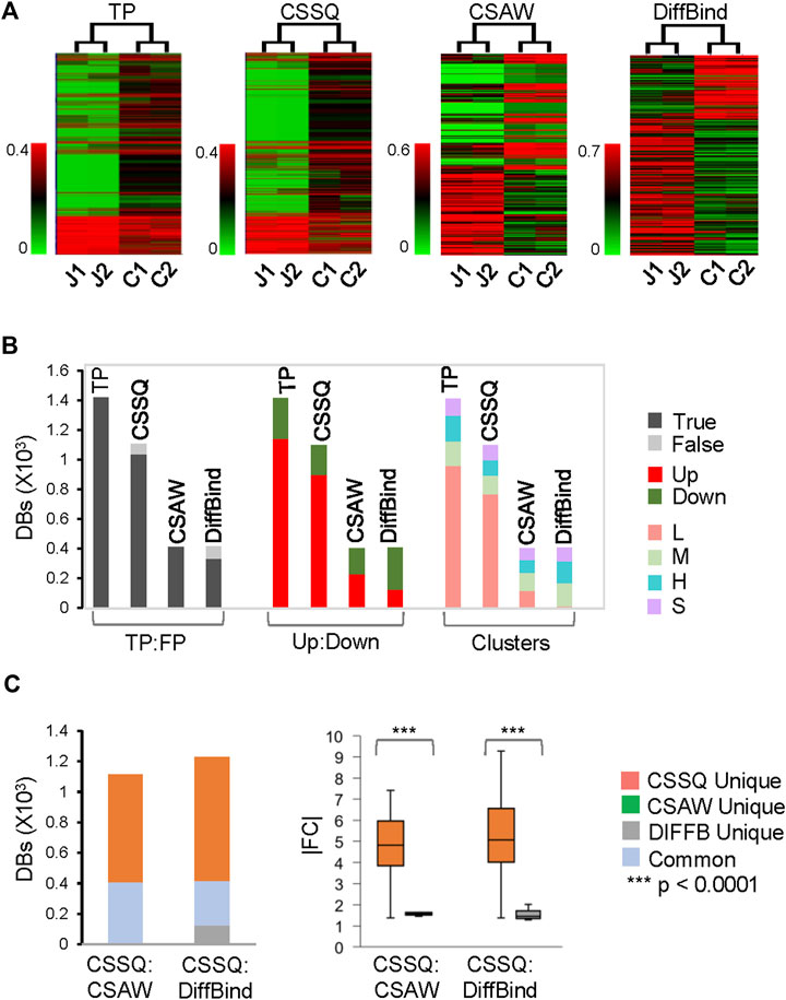
FIGURE 5. DB analysis on representative simulated simhESC-1 datasets. 2.5% of data points were induced as DBs. Randomly sampled Usim factors from KDE were 59.2 (J1), 56.0 (J2), 53.0 (C1) and 56.0 (C2). (A) hierarchical clustering of DBs. (B) DB distributions. TP: True Positive; FP: False Positive. (C) DB comparisons by CSSQ vs. CSAW and CSSQ vs. DiffBind.
We next tested CSSQ performance on real ChIP-seq datasets of H3K4me3 and H3K27me3, two characteristic histone marks with typical sharp and broad peaks, respectively (Benayoun et al., 2014; Cai et al., 2021). Toward this end, we analyzed four well-characterized cell lines, including two human cell lines of different cell types, the H1 hESC cell line and the K562 myeloid leukemia cell line, as well as two highly similar mouse ESC cell lines, the wild-type (WT) and H1c/H1d/H1e triple knockout (TKO) ESCs (Fan et al., 2005; Consortium, 2011; Geeven et al., 2015). H3K4me3 signals were analyzed for gene promoter regions flanking TSS, whereas H3K27me3 signals were compared for H3K27me3-rich regions [designated as “MRRs” or “super silencers” (Cai et al., 2021)]. The signals of H3K4me3 at gene promoters positively correlate with gene expression levels, thus transcriptome profiles of differentially expressed genes (DEGs) were included as measurement controls for DB detection of H3K4me3 at promoters. For H3K27me3 analysis, DB detection was performed for K562 MRRs, including “all K562 MRRs,” “K562 only MRRs” (K562 MRRs excluding overlapping hESC MRRs) and “K562-hESC overlapping MRRs”.
CSSQ identified 9,423 and 447 H3K4me3 DBs with in K562/hESC and TKO/WT comparisons. Such dramatic differences in the number of DBs detected in K562/hESC and TKO/WT comparisons mimicking the differences of DEGs in corresponding transcriptome analyses (Figure 6). hESCs and K562 cells exhibited distinctively gene expression profiles with 11,197 DEGs, whereas WT and H1 TKO ESCs had minimal gene expression changes, with only 27 DEGs of 2-fold changes from RNAseq analysis (Figure 6), consistent with previous findings (Fan et al., 2005; Geeven et al., 2015; Pan and Fan, 2016). CSSQ identified DBs were also in similar up/down trend to DEGs for both K562/hESC and TKO/WT comparisons, with upregulated DBs accounting for a minority, 22% in K562/hESC, and a majority, 82% in TKO/WT comparisons (Figure 6). CSAW detected comparable numbers of Up/Down DBs for K562/hESC, and DiffBind found 2,262 DBs for TKO/WT with only <3% being upregulated, in striking contrast to the characteristic profiles of TKO/WT DEGs of limited number and a majority (67%) as upregulated (Figure 6).
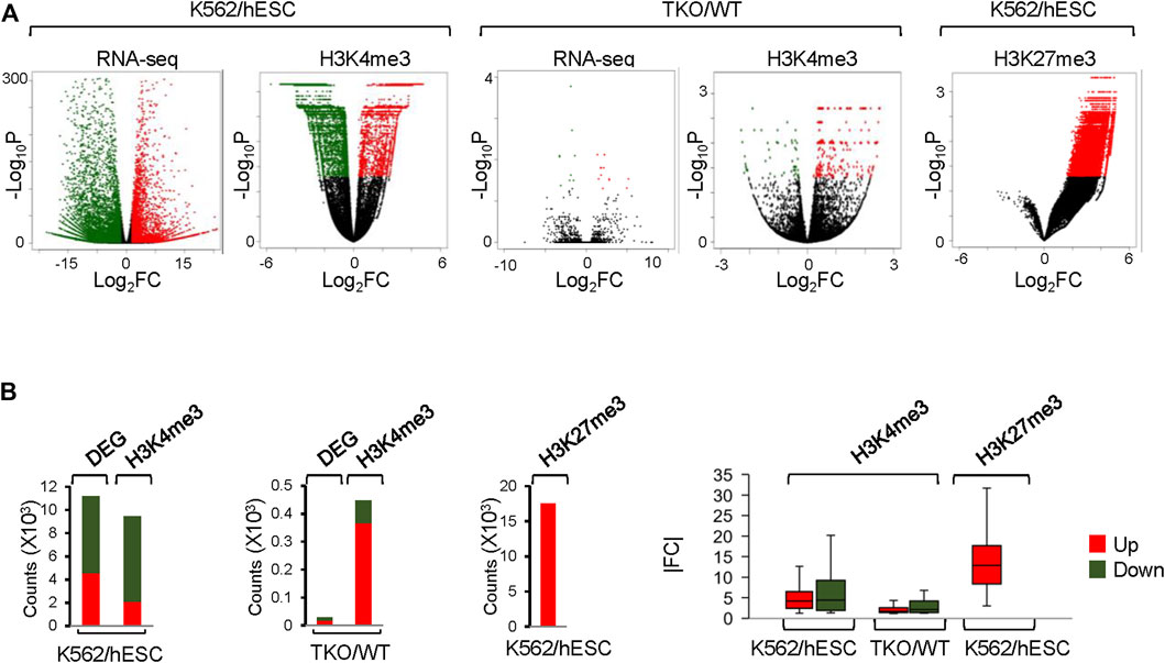
FIGURE 6. Analysis of DEGs and CSSQ DBs on real ChIP-seq datasets. (A) Volcano plots showing DBs and DEGs Identified in H3K4me3 and H3K27me3 datasets. Upregulated and downregulated datapoints (p < 0.05) are marked in red and green respectively. (B) bar plots of DB and DEG counts and |FC| of identified upregulated (Up) and downregulated (Down) DBs.
Metagene profiling of IP-IN signals of H3K4me3 CSSQ DBs partitioned in clusters revealed a clear difference in the signal levels of increasing signal intensity in L, M, H, and S clusters across regions flanking TSS (Supplementary Figure S7). CSSQ DBs in clusters also followed the trend of up/down proportion of DEGs and exhibited pronounced signal differences in normalized (IP-IN)* values (Figure 6, Figure 7, Supplementary Figure S8). The average |FC| for CSSQ H3K4me3 DBs were 6.2 in K562/hESC and 2.4 in TKO/WT (Supplementary Figure S9). The higher average |FC| in K562/hESC DBs than that of TKO/WT is also observed in up/downregulated DB groups and in each cluster, consistent with expected trend from DEG profiling (Figure 6, Supplementary Figure S9). In comparison, CSAW and DiffBind DBs had lower |FC| values, at 1.8 and 1.1, in TKO/WT, respectively (data not shown).
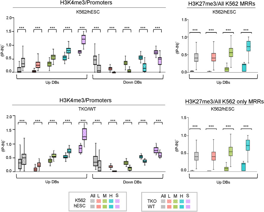
FIGURE 7. Box plots of CSSQ normalized signals for DBs in different clusters identified using CSSQ analysis of real ChIP-seq datasets. Left: comparisons of H3K4me3 ChIP-seq datasets from human K562 vs. hESC cells and mouse TKO vs WT cells over promoter regions (TSS ± 1 kb); Right: comparisons of H3K27me3 ChIP-seq datasets from human K562 vs. hESC cells over all K562 MRR regions and over K562 only MRR regions. ***p < 0.0001.
CSSQ performance on DB detection and quantification of broad peaks such as H3K27me3 was also robust. For K562/hESC analysis, among 41,948 “all K562 MRRs” and 35,023 “K562 only MRRs”, CSSQ identified 17,552 and 16,554 DBs, respectively, and all (100%) of the CSSQ DBs were upregulated (Up DBs) (Figure 6B, Supplementary Figure S8), validating these regions being K562 MRRs as reported (Cai et al., 2021). The CSSQ H3K27me3 DBs were mostly concentrated in the “L” cluster (Supplementary Figure S8). DB Profiling showed a clear difference in the normalized (IP-IN)* signal levels of CSSQ DBs and the average |FC| for DBs identified in each cluster (Figure 7, Supplementary Figure S9). In contrast, CSAW and DiffBind found fewer DBs among “all K562 MRRs” and “K562 only MRRs”, and both CSAW and DiffBind had downregulated DBs even in “K562 only MRRs” despite these MRRs barring H3K27me3 enriched regions in hESCs (i.e., free of hESC MRRs) (Figure 8A). Hierarchical clustering for DBs clustered the replicates together for all three pipelines (Supplementary Figure S10).
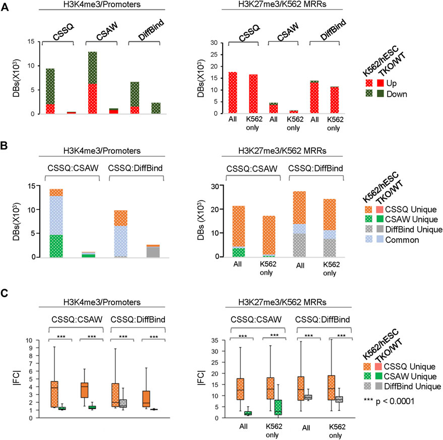
FIGURE 8. In depth analysis and comparisons of DBs detected by CSSQ, CSAW, and DiffBind on real ChIP-seq datasets. (A) Counts of Up and Downregulated DBs. (B) Counts of unique and common DBs identified using each tool from pair-wise comparisons. (C) |FC| of unique DBs identified using each tool from pair-wise comparisons. Labels for H3K27me3 dataset—All: all K562 MRRs; K562 only: K562 only MRRs.
To further evaluate the DBs detected by all three pipelines, we performed pairwise comparisons and scrutinized the common and unique DBs to each pipeline. For H3K4me3 K562/hESC comparison, 8,065 common DBs were detected in CSSQ vs CSAW and 6,243 common DBs were called in CSSQ vs DiffBind, whereas TKO/WT H3K4me3 analysis resulted in 400 (CSSQ vs CSAW) and 83 (CSSQ vs DiffBind) common DBs (Figure 8B). A representative common K562/hESC DB was detected at the site of GATA1, the transcription factor markedly upregulated in K562 cells, and this locus exhibited robust signal in K562 as expected (Figure 9A). H1d gene promoter region was among the 400 (CSSQ vs CSAW) common DBs, lacking signals in TKO cells (Figure 9A), consistent with the deletion of H1d gene and its promoter region during H1d gene targeting (Fan et al., 2001; Fan et al., 2005). DiffBind did not detect H1d as a DB. For H3K27me3 DB analysis of K562/hESC at K562 MRRs, 705 and 4,009 common DBs were detected in CSSQ vs. CSAW and CSSQ vs. DiffBind, respectively (Figure 8B).
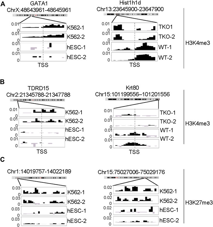
FIGURE 9. ChIP-seq signal profiles at representative loci. (A) H3K4me3 ChIP-seq signal profile around TSS of representative gene loci of DBs identified from K562 vs. hESC (left) and H1 TKO vs. WT (right) comparisons. (B, C) Representative H3K4me3 and H3K27me3 ChIP-seq signal profiles of unique DB regions identified by CSSQ in K562 vs. hESC comparisons.
The average |FC| of CSSQ unique DBs were statistically higher (p < 0.0001) than those of CSAW and DiffBind in all pair-wise comparisons (Figure 8C). Visual inspection of individual CSSQ unique DBs also validated bona fide signal enrichment of H3K4me3 and H3K27me3 peaks as the DB regions (Figures 9B, C). For H3K4me3 DBs, when compared with CSAW, unique CSSQ DBs had an average |FC| of 3.6 (K562/hESC) and 3.7 (TKO/WT) while that of CSAW displayed 1.4 FC (K562/hESC) and 1.5 FC (TKO/WT) (Figure 8C). Similarly, the |FC| of unique CSSQ DBs were significantly higher than that of DiffBind unique DBs (Figure 8C). The |FC| difference of unique CSSQ DBs was even more prominent when H3K27me3 K562/hESC DBs were gauged. From “all K562 MRRs” analysis, unique CSSQ DBs had mean |FC| at 13.6 and 13.9 as compared with that of unique DBs of CSAW and DiffBind at 2.6 and 7.3 from CSSQ vs. CSAW and CSSQ vs. DiffBind comparisons, respectively (Figure 8C). A similar trend was observed with DB analysis on “K562only MRRs” and “K562/hESC overlapping MRRs” (Supplementary Figure S11).
ChIP-seq has revolutionized the mapping of DNA binding proteins across genome in vivo. The massive increase in the amount of data being generated from ChIP-seq and related methods demands robust computational tools that allow for detection and quantitation of genome-wide protein binding (Schmidl et al., 2015; Visa and Jordan-Pla, 2018). However, powerful pipelines capable of direct quantitation of ChIP-seq signals across different datasets are in short supply (Steinhauser et al., 2016; Nakato and Sakata, 2021). By employing sophisticated statistical approaches, we developed CSSQ, an innovative ChIP-seq signal quantifier that is capable of detection and quantitation of interesting regions with high confidence and sensitivity.
CSSQ fits a Gaussian mixture model to the transformed data instead of fitting a single distribution such as the negative binomial distribution to the raw count data. It utilizes a combination of Anscombe transformation, k-means clustering, and estimated maximum normalization to minimize noise and bias from experimental variations. Anscombe transformation effectively converts ChIP-seq raw data from an approximate mixture of Poisson distributions (Supplementary Figure S12) into Gaussian mixture models. Our choice of k clustering into 4 groups here is based on extensive tests and analyses. We find that k = 4 in general balances the goodness-of-fit and model complexity of datasets tested. As illustrated in the representative scree plots generated on “Variance Explained” (within-in cluster variance) and “Adjusted R-squared” (between-cluster variance) with respect to different number of clusters (Supplementary Figure S13), based on the elbow method, k = 4 represents a bend position and a robust number of clusters, e.g., the improvement from k-3 to k = 4 is still relatively large (4%), while the improvement from k = 4 to k = 5 (2%) turns to relatively small. In addition, this clustering partitions the data points into 4 well-defined, biologically meaningful data groups representing low (L), medium (M), high (H), super high (S) signals, respectively.
To statistically test significance and DB calling, CSSQ utilizes a non-parametric approach and incorporates comparisons under the null hypothesis by re-shuffling datasets among different groups to perform robust statistical tests to account for fewer replicates of ChIP-seq datasets of the same biological samples. It reports an adjusted p-value and a fold-change (FC) for all pre-defined regions. The normalization method adopted in CSSQ and the generation of comparisons under the null hypothesis by re-shuffling of datasets for DB calling are novel applications of mathematical treatments to ChIP-seq datasets. These approaches employed by CSSQ play a critical role in reducing false DB calls that may arise due to experimental noises and biases.
Using simulation studies and quantitative metrics, we benchmarked CSSQ with the CSAW and DiffBind pipelines. CSSQ identified induced DBs with a low FDR and high sensitivity under all simulation scenarios. While CSAW had a slightly lower FDR than CSSQ, its sensitivity was not consistent and much lower than CSSQ in nearly all simulations (Figure 4). Even though DiffBind occasionally had similar sensitivity as CSSQ in DB calls, such as in simhESC-2 simulations, it consistently had a higher FDR (Figure 4). CSSQ exhibited the highest power and robustness in distinguishing between true and false DBs, as evidenced from its ROC curves and the highest AUCs in all simulations. Further, in our in-depth analysis of a simulated dataset, unique DBs identified by CSSQ had a higher |FC| with statistical significance (p < 0.0001) when compared to those of CSAW and DiffBind, suggesting that unique DBs of CSSQ are more likely to be true DBs than those of CSAW and DiffBind (Figure 5C). The results were consistent in both simulation studies, one analyzing the performance on different percentages of true DBs and the other on different magnitudes of signal differences in DBI. The results from these simulations demonstrate the robustness of the CSSQ pipeline.
CSSQ also outperforms parallel pipelines in benchmarking exercises using real ChIP-seq datasets. K562 human multipotent leukemia cell line and H1 human pluripotent embryonic stem cell line are two distinct cell types with 11,197 DEGs that accounts for nearly 20% of all genes in the human genome. While ChIP-seq analysis of promoter H3K4me3 reflected this well with all three tools identifying thousands of potential DBs. including various cell specific marker genes, unique DBs from CSSQ had a higher |FC| when compared with those from CSAW and DiffBind. In addition to comparison test using ChIP-seq datasets from entirely different cell types, we also scrutinized DBs detected by the three pipelines on datasets from two highly similar cell lines, mouse H1 TKO and WT ESCs that had very limited gene expression changes at undifferentiated states (Fan et al., 2005). Transcriptome analysis of RNAseq datasets from TKO/WT comparisons only identified 27 statistically significant DEGs (Geeven et al., 2015), and CSSQ had the least number of DBs from analysis of the TKO/WT H3K4me3 ChIP-seq datasets among the three pipelines (Figures 6, 8).
To robustly compare the performance of the pipelines on different signal profiles, we further benchmarked using H3K27me3 ChIP-seq data which exhibit a broad signal profile. Utilizing H3K27me3-rich regions (MRR) in K562 and hESC (Cai et al., 2021), again we found that CSSQ has a higher sensitivity in identifying DBs than CSAW and DiffBind (Figures 6, 8).
CSSQ and DiffBind were designed to analyze predefined regions of interests. DiffBind uses statistical routines developed for RNAseq (DESeq2 (Love et al., 2014) and EdgeR (Robinson et al., 2010)) to identify significant DB regions (Ross-Innes et al., 2012). CSAW was primarily designed for genome-wide de novo detection of DB regions between samples using statistical tests implemented in edgeR. CSAW, like DiffBind, utilizes statistical testing methods that were developed for differential gene expression analysis in EdgeR package (Robinson et al., 2010; Lun and Smyth, 2016). The inherent difference between the data distribution of ChIP-seq and RNAseq datasets and the use of control libraries for background correction in ChIP-seq make it less ideal to apply the same statistical approach for RNAseq on ChIP-seq datasets (Figure 1B, Supplementary Figures S1, S14).
In summary, the CSSQ pipeline is a statistically robust pipeline to perform differential binding analysis on pre-defined regions of interest across ChIP-seq samples. It enables quantitative analysis of ChIP-seq data by utilizing statistically sound methods to normalize for experimental biases, control false discovery rate and provide high confidence DB calls and quantification.
CSSQ is implemented as an R package available in open-source form at http://bioconductor.org/packages/release/bioc/html/CSSQ.html and https://github.com/fan-lab-gatech. The datasets used in this study can be found in online repositories. The names of the repository/repositories and accession number(s) can be found in the article/Supplementary Material.
AK and YF contributed to conception, study design, and carried out the investigation. YF acquired funding, resources and directed the project. MH and YM contributed to methodology and statistical analysis. AK, YM, and YF wrote the original draft, and MH contributed to writing sections of the manuscript. All authors contributed to the article and approved the submitted version.
This work is in part supported by NSF STC for Emergent Behaviors of Integrated Cellular Systems (EBICS) (Award #: CBET0939511), Georgia Partners in Regenerative Medicine, Nelson and Bennie Abell Professorship in Biology (to YF), and Georgia Institute of Technology. The funders had no role in study design, data collection and analysis, decision to publish, or preparation of the manuscript.
The authors thank the open-source Bioconductor and GitHub for supporting CSSQ, Yunzhe Zhang for editorial assistance, and colleagues for helpful feedback.
The authors declare that the research was conducted in the absence of any commercial or financial relationships that could be construed as a potential conflict of interest.
All claims expressed in this article are solely those of the authors and do not necessarily represent those of their affiliated organizations, or those of the publisher, the editors and the reviewers. Any product that may be evaluated in this article, or claim that may be made by its manufacturer, is not guaranteed or endorsed by the publisher.
The Supplementary Material for this article can be found online at: https://www.frontiersin.org/articles/10.3389/fcell.2023.1167111/full#supplementary-material
Allis, C. D., and Jenuwein, T. (2016). The molecular hallmarks of epigenetic control. Nat. Rev. Genet. 17, 487–500. doi:10.1038/nrg.2016.59
Anders, S., Pyl, P. T., and Huber, W. (2015). HTSeq-a Python framework to work with high-throughput sequencing data. Bioinformatics 31, 166–169. doi:10.1093/bioinformatics/btu638
Andrews, S. (2022). bioinformatics. Avaliable At: https://www.bioinformatics.babraham.ac.uk/projects/fastqc/.
Anscombe, F. J. (1948). The transformation of Poisson, binomial and negative-binomial data. Biometrika 35, 246–254. doi:10.1093/biomet/35.3-4.246
Barski, A., Cuddapah, S., Cui, K., Roh, T. Y., Schones, D. E., Wang, Z., et al. (2007). High-resolution profiling of histone methylations in the human genome. Cell. 129, 823–837. doi:10.1016/j.cell.2007.05.009
Benayoun, B. A., Pollina, E. A., Ucar, D., Mahmoudi, S., Karra, K., Wong, E. D., et al. (2014). H3K4me3 breadth is linked to cell identity and transcriptional consistency. Cell. 158, 673–688. doi:10.1016/j.cell.2014.06.027
Benjamini, Y., and Hochberg, Y. (1995). Controlling the false discovery rate: A practical and powerful approach to multiple testing. J. R. Stat. Soc. Ser. B Methodol. 57, 289–300. doi:10.1111/j.2517-6161.1995.tb02031.x
Cai, Y., Zhang, Y., Loh, Y. P., Tng, J. Q., Lim, M. C., Cao, Z., et al. (2021). H3K27me3-rich genomic regions can function as silencers to repress gene expression via chromatin interactions. Nat. Commun. 12, 719–722. doi:10.1038/s41467-021-20940-y
Cao, K., Lailler, N., Zhang, Y., Kumar, A., Uppal, K., Liu, Z., et al. (2013). High-resolution mapping of h1 linker histone variants in embryonic stem cells. PLoS Genet. 9, e1003417. doi:10.1371/journal.pgen.1003417
Chen, L., Wang, C., Qin, Z. S., and Wu, H. (2015). A novel statistical method for quantitative comparison of multiple ChIP-seq datasets. Bioinformatics 31, 1889–1896. doi:10.1093/bioinformatics/btv094
Consortium, E. P. (2011). A user's guide to the encyclopedia of DNA elements (ENCODE). PLoS Biol. 9, e1001046. doi:10.1371/journal.pbio.1001046
Dobin, A., Davis, C. A., Schlesinger, F., Drenkow, J., Zaleski, C., Jha, S., et al. (2013). Star: Ultrafast universal RNA-seq aligner. Bioinformatics 29, 15–21. doi:10.1093/bioinformatics/bts635
Eder, T., and Grebien, F. (2022). Comprehensive assessment of differential ChIP-seq tools guides optimal algorithm selection. Genome Biol. 23, 119–127. doi:10.1186/s13059-022-02686-y
Fan, Y., Nikitina, T., Zhao, J., Fleury, T. J., Bhattacharyya, R., Bouhassira, E. E., et al. (2005). Histone H1 depletion in mammals alters global chromatin structure but causes specific changes in gene regulation. Cell. 123, 1199–1212. doi:10.1016/j.cell.2005.10.028
Fan, Y., Sirotkin, A., Russell, R. G., Ayala, J., and Skoultchi, A. I. (2001). Individual somatic H1 subtypes Are dispensable for mouse development even in mice lacking the H10Replacement subtype. Mol. Cell. Biol. 21, 7933–7943. doi:10.1128/MCB.21.23.7933-7943.2001
Geeven, G., Zhu, Y., Kim, B. J., Bartholdy, B. A., Yang, S. M., Macfarlan, T. S., et al. (2015). Local compartment changes and regulatory landscape alterations in histone H1-depleted cells. Genome Biol. 16, 289. doi:10.1186/s13059-015-0857-0
Heintzman, N. D., Stuart, R. K., Hon, G., Fu, Y., Ching, C. W., Hawkins, R. D., et al. (2007). Distinct and predictive chromatin signatures of transcriptional promoters and enhancers in the human genome. Nat. Genet. 39, 311–318. doi:10.1038/ng1966
Hollbacher, B., Balazs, K., Heinig, M., and Uhlenhaut, N. H. (2020). Seq-ing answers: Current data integration approaches to uncover mechanisms of transcriptional regulation. Comput. Struct. Biotechnol. J. 18, 1330–1341. doi:10.1016/j.csbj.2020.05.018
Howe, E. A., Sinha, R., Schlauch, D., and Quackenbush, J. (2011). RNA-Seq analysis in MeV. Bioinformatics 27, 3209–3210. doi:10.1093/bioinformatics/btr490
Jambhekar, A., Dhall, A., and Shi, Y. (2019). Roles and regulation of histone methylation in animal development. Nat. Rev. Mol. Cell. Biol. 20, 625–641. doi:10.1038/s41580-019-0151-1
Jeon, H., Lee, H., Kang, B., Jang, I., and Roh, T. Y. (2020). Comparative analysis of commonly used peak calling programs for ChIP-Seq analysis. Genomics Inf. 18, e42. doi:10.5808/GI.2020.18.4.e42
Johnson, D. S., Mortazavi, A., Myers, R. M., and Wold, B. (2007). Genome-wide mapping of in vivo protein-DNA interactions. Science 316, 1497–1502. doi:10.1126/science.1141319
Krueger, F. (2021). bioinformatics. Avaliable At: https://www.bioinformatics.babraham.ac.uk/projects/trim_galore/.
Lajugie, J., and Bouhassira, E. E. (2011). GenPlay, a multipurpose genome analyzer and browser. Bioinformatics 27, 1889–1893. doi:10.1093/bioinformatics/btr309
Lajugie, J., Fourel, N., and Bouhassira, E. E. (2015). GenPlay Multi-Genome, a tool to compare and analyze multiple human genomes in a graphical interface. Bioinformatics 31, 109–111. doi:10.1093/bioinformatics/btu588
Langmead, B., Trapnell, C., Pop, M., and Salzberg, S. L. (2009). Ultrafast and memory-efficient alignment of short DNA sequences to the human genome. Genome Biol. 10, R25. doi:10.1186/gb-2009-10-3-r25
Li, H., Handsaker, B., Wysoker, A., Fennell, T., Ruan, J., Homer, N., et al. (2009). The sequence alignment/map format and SAMtools. Bioinformatics 25, 2078–2079. doi:10.1093/bioinformatics/btp352
Liang, K., and Keles, S. (2012). Detecting differential binding of transcription factors with ChIP-seq. Bioinformatics 28, 121–122. doi:10.1093/bioinformatics/btr605
Love, M. I., Huber, W., and Anders, S. (2014). Moderated estimation of fold change and dispersion for RNA-seq data with DESeq2. Genome Biol. 15, 550. doi:10.1186/s13059-014-0550-8
Lun, A. T., and Smyth, G. K. (2016). csaw: a Bioconductor package for differential binding analysis of ChIP-seq data using sliding windows. Nucleic Acids Res. 44, e45. doi:10.1093/nar/gkv1191
Lun, A. T., and Smyth, G. K. (2014). De novo detection of differentially bound regions for ChIP-seq data using peaks and windows: Controlling error rates correctly. Nucleic acids Res. 42, e95. doi:10.1093/nar/gku351
Martin, M. (2011). Cutadapt removes adapter sequences from high-throughput sequencing reads. EMBnet. J. 17, 10–12. doi:10.14806/ej.17.1.200
Mundade, R., Ozer, H. G., Wei, H., Prabhu, L., and Lu, T. (2014). Role of ChIP-seq in the discovery of transcription factor binding sites, differential gene regulation mechanism, epigenetic marks and beyond. Cell. Cycle 13, 2847–2852. doi:10.4161/15384101.2014.949201
Nakato, R., and Sakata, T. (2021). Methods for ChIP-seq analysis: A practical workflow and advanced applications. Methods 187, 44–53. doi:10.1016/j.ymeth.2020.03.005
Pan, C., and Fan, Y. (2016). Role of H1 linker histones in mammalian development and stem cell differentiation. Biochim. Biophys. Acta 1859, 496–509. doi:10.1016/j.bbagrm.2015.12.002
Park, P. J. (2009). ChIP-seq: Advantages and challenges of a maturing technology. Nat. Rev. Genet. 10, 669–680. doi:10.1038/nrg2641
Quinlan, A. R., and Hall, I. M. (2010). BEDTools: A flexible suite of utilities for comparing genomic features. Bioinformatics 26, 841–842. doi:10.1093/bioinformatics/btq033
Robinson, M. D., Mccarthy, D. J., and Smyth, G. K. (2010). edgeR: a Bioconductor package for differential expression analysis of digital gene expression data. Bioinformatics 26, 139–140. doi:10.1093/bioinformatics/btp616
Ross-Innes, C. S., Stark, R., Teschendorff, A. E., Holmes, K. A., Ali, H. R., Dunning, M. J., et al. (2012). Differential oestrogen receptor binding is associated with clinical outcome in breast cancer. Nature 481, 389–393. doi:10.1038/nature10730
Schmidl, C., Rendeiro, A. F., Sheffield, N. C., and Bock, C. (2015). ChIPmentation: Fast, robust, low-input ChIP-seq for histones and transcription factors. Nat. Methods 12, 963–965. doi:10.1038/nmeth.3542
Shen, L., Shao, N. Y., Liu, X., Maze, I., Feng, J., and Nestler, E. J. (2013). diffReps: detecting differential chromatin modification sites from ChIP-seq data with biological replicates. PLoS One 8, e65598. doi:10.1371/journal.pone.0065598
Shen, Y., Yue, F., Mccleary, D. F., Ye, Z., Edsall, L., Kuan, S., et al. (2012). A map of the cis-regulatory sequences in the mouse genome. Nature 488, 116–120. doi:10.1038/nature11243
Stark, R., and Brown, G. (2011). DiffBind: Differential binding analysis of ChIP-seq peak data. Avaliable At: http://bioconductor.org/packages/release/bioc/vignettes/DiffBind/inst/doc/DiffBind.pdf.
Steinhauser, S., Kurzawa, N., Eils, R., and Herrmann, C. (2016). A comprehensive comparison of tools for differential ChIP-seq analysis. Brief. Bioinform 17, 953–966. doi:10.1093/bib/bbv110
Tu, S., and Shao, Z. (2017). An introduction to computational tools for differential binding analysis with ChIP-seq data. Quant. Biol. 5, 226–235. doi:10.1007/s40484-017-0111-8
Visa, N., and Jordan-Pla, A. (2018). ChIP and ChIP-related techniques: Expanding the fields of application and improving ChIP performance. Methods Mol. Biol. 1689, 1–7. doi:10.1007/978-1-4939-7380-4_1
Zang, C., Schones, D. E., Zeng, C., Cui, K., Zhao, K., and Peng, W. (2009). A clustering approach for identification of enriched domains from histone modification ChIP-Seq data. Bioinformatics 25, 1952–1958. doi:10.1093/bioinformatics/btp340
Zhang, Y., Lin, Y. H., Johnson, T. D., Rozek, L. S., and Sartor, M. A. (2014). PePr: A peak-calling prioritization pipeline to identify consistent or differential peaks from replicated ChIP-seq data. Bioinformatics 30, 2568–2575. doi:10.1093/bioinformatics/btu372
Zhang, Y., Liu, T., Meyer, C. A., Eeckhoute, J., Johnson, D. S., Bernstein, B. E., et al. (2008). Model-based analysis of ChIP-seq (MACS). Genome Biol. 9, R137. doi:10.1186/gb-2008-9-9-r137
Keywords: ChIP-seq signal quantifier (CSSQ), ChIP-seq, differential binding, epigenetic marks, statistical analysis, k-means clustering, normalization, Gaussian mixture model
Citation: Kumar A, Hu MY, Mei Y and Fan Y (2023) CSSQ: a ChIP-seq signal quantifier pipeline. Front. Cell Dev. Biol. 11:1167111. doi: 10.3389/fcell.2023.1167111
Received: 16 February 2023; Accepted: 02 May 2023;
Published: 25 May 2023.
Edited by:
Pao-Yang Chen, Academia Sinica, TaiwanReviewed by:
Yu-Wei Wu, Taipei Medical University, TaiwanCopyright © 2023 Kumar, Hu, Mei and Fan. This is an open-access article distributed under the terms of the Creative Commons Attribution License (CC BY). The use, distribution or reproduction in other forums is permitted, provided the original author(s) and the copyright owner(s) are credited and that the original publication in this journal is cited, in accordance with accepted academic practice. No use, distribution or reproduction is permitted which does not comply with these terms.
*Correspondence: Yuhong Fan, eXVob25nLmZhbkBiaW9sb2d5LmdhdGVjaC5lZHU=
†Present address: Michael Y. Hu, Center for Data Science, New York University, New York, NY, United States
Disclaimer: All claims expressed in this article are solely those of the authors and do not necessarily represent those of their affiliated organizations, or those of the publisher, the editors and the reviewers. Any product that may be evaluated in this article or claim that may be made by its manufacturer is not guaranteed or endorsed by the publisher.
Research integrity at Frontiers
Learn more about the work of our research integrity team to safeguard the quality of each article we publish.